SGIR-Tree: Integrating R-Tree Spatial Indexing as Subgraphs in Graph Database Management Systems

Abstract

Efficient spatial query processing in Graph Database Management Systems (GDBMSs) has become increasingly important owing to the prevalence of spatial graph data. However, current GDBMSs lack effective spatial indexing, causing performance issues with complex spatial graph queries. This study proposes a spatial index called Subgraph Integrated R-Tree (SGIR-Tree) for efficient spatial query processing in GDBMSs. The SGIR-Tree integrates the hierarchical R-Tree structure with the graph structure of GDBMSs by converting R-Tree elements into graph components like nodes and edges. The Minimum Bounding Rectangle (MBR) information of spatial objects and R-Tree nodes is stored as properties of these graph elements, and the leaf nodes are directly connected to the spatial nodes. This approach combines the efficiency of spatial indexing with the flexibility of graph databases, thereby allowing spatial query results to be directly utilized in graph traversal. Experiments using OpenStreetMap datasets demonstrate that the SGIR-Tree outperforms the previous approaches in terms of query overhead and index overhead. The results are expected to improve spatial graph data processing in various fields, including location-based service and urban planning, significantly advancing spatial data management in GDBMSs.

1. Introduction

Spatial indices are crucial in database systems for efficiently managing geospatial data and optimizing spatial query processing [1,2], which is essential for applications such as location-based services, urban planning, and GIS. With the increased use of graphs to manage and analyze large and complex spatial data [3,4,5,6], spatial indices in Graph Database Management Systems (GDBMSs) have become more important. A spatial index creates a specific order and arrangement for spatial objects, which facilitates the rough filtering of unnecessary data during spatial queries and aids in quickly finding target objects [7]. In GDBMSs, where complex queries often require both spatial search and graph traversal, the lack of an effective spatial index can render even simple queries computationally expensive, thereby severely affecting performance [8]. For example, a spatial join query between two large spatial object sets exhibits a complexity of $O\left(N^2\right)$ without a spatial index, where N is the number of spatial objects. However, using an efficient spatial index such as R-Tree, this can be reduced to $O\left(lo{g}_{M}N\right)$ on average, where M is the capacity of each node in the R-Tree, representing the maximum number of children it can contain. This improvement is crucial for managing large-scale geospatial graph data efficiently.

Despite the importance of spatial indices, many GDBMSs do not support spatial indexing, thereby degrading the performance of spatial queries. Even when certain GDBMSs, such as Blazegraph, support spatial indexing, they often provide limited spatial queries [9]. Spatial queries refer to various spatial operations on objects within the database, such as spatial join (topological relationships) and K-nearest neighbors (KNN) [10]. Furthermore, they tend to support space-driven indices, which have approximation errors, rather than data-driven structures like R-Tree or Quad-Tree. Few DBMSs are specifically designed for geospatial graphs. Specifically, most GDBMSs handle spatial functions and indices through plugins or libraries [8]. These approaches differ based on whether the spatial index is stored outside or inside the GDBMS. If stored internally, it might be managed as an isolated graph separate from the entire graph or as an integrated subgraph. However, managing the spatial index as an isolated graph within the GDBMS leads to overhead when integrating the results of spatial queries into the GDBMS. Similarly, storing the spatial index externally can cause overhead because the index needs to be loaded and processed separately from the GDBMS operations.

In Figure 1, the upper graph represents a geospatial social network that shows the relationships and visited locations of people on SNS, and the lower graph represents an R-Tree index depicted with gray rectangles. For example, let us assume that David is currently visiting the Empire State Building. And he is looking for a restaurant within 500 m (Green Circle) that Alice, whom he follows on SNS, has visited. If the spatial index is disconnected from the entire graph (Figure 1a), spatial entities within 500 m can be found (green map marker), but matching the restaurant within the entire graph is required. However, if the spatial index is configured as a subgraph connected to the entire graph (Figure 1b), restaurants within 500 m can be directly identified, and graph traverse can be used to find the specific restaurant, “Bonchon”, visited by Alice.

Currently, several GDBMS spatial plugins or libraries fail to effectively integrate spatial indices with graph structures, resulting in inefficient spatial graph queries. Although some studies address handling both spatial and graph constraints in GDBMSs, they often show scalability limitations with complex or large data [8,11]. Thus, there is a lack of optimized index structures for efficiently processing complex queries that involve both spatial searches and graph traversals; this renders it challenging to process and analyze spatial data efficiently in GDBMSs, potentially causing performance bottlenecks in applications that handle large-scale geospatial graph data.

In this context, this study proposes a spatial index, that is, the Subgraph Integrated R-Tree (SGIR-Tree), that connects the spatial index to the entire graph as a subgraph, which renders it suitable for use in GDBMSs. The proposed index converts the nodes of the R-Tree into nodes of the graph, and the pointers of the R-Tree into edges of the graph, and stores the Minimum Boundary Rectangle (MBR) of the R-Tree as properties of the graph nodes and edges. It also directly connects the leaf nodes of the R-Tree to the spatial nodes within the GDBMSs. This index configuration aims to eliminate the matching overhead between spatial entities by the spatial index and those in the entire graph, thereby improving the efficiency of spatial queries within the GDBMS.

The contributions of this study are as follows:

• We propose a new index structure named SGIR-Tree, which integrates spatial index components as a subgraph based on representative spatial index R-Tree. This integration minimizes the I/O overhead and improves index management, thereby providing a more efficient and scalable solution for spatial indexing within GDBMS environments.
• We enhance query processing capabilities by seamlessly integrating spatial and graph queries. This integration facilitates more efficient handling of complex queries that require both spatial search and graph traversal.
• We implement and test the SGIR-Tree in a widely used GDBMS, Neo4j, demonstrating its effectiveness with various spatial data types and queries such as spatial join, KNN, and spatial range. The experiments conducted show that the SGIR-Tree outperforms both disconnected spatial indices stored within the GDBMS and externally stored spatial indices for spatial graph queries.

The remainder of this paper is structured as follows. Section 2 reviews the existing approaches to spatial indexing in GDBMSs, highlighting current limitations and challenges. Section 3 presents the proposed SGIR-Tree, detailing its index structure design, initialization and maintenance methods, and spatial query processing algorithms. Section 4 describes the experimental setup and presents a comprehensive evaluation of the SGIR-Tree performance. Comparisons are made with existing approaches. Finally, Section 5 summarizes the key contributions and discusses potential future research directions.

2. Related Work

This section reviews previous studies on spatial indexing in GDBMSs. First, we introduce the basic types and characteristics of spatial indices to explain the fundamentals of spatial indexing. Next, we examine the implementation and usage of spatial indices in GDBMSs, categorizing them into RDF and LPG models. Finally, we summarize the limitations of previous studies and present the approach of this study.

2.1. Type of Spatial Index

Spatial indices can be broadly classified into two types based on the strategy for partitioning spatial objects: data-driven partitioning and space-driven partitioning [2].

First, the data-driven partitioning strategy partitions space according to the spatial objects. Indices using this strategy include the R-Tree [12] series and the K-D Tree [13] series. The R-Tree approximates various types of spatial objects using MBRs and clusters them into leaf nodes based on the proximity of the MBRs, forming a hierarchical tree. Several variations of the R-Tree have been developed, such as the R+-Tree [14], which eliminates MBR overlap in leaf nodes by facilitating the duplicate storage of spatial objects’ MBRs, and the R*-Tree [15], which improves the efficiency of index nodes’ MBRs by considering the overlap between leaf nodes using a clustering parameter. The K-D Tree partitions space based on point-type spatial objects, forming a binary tree. Notable variants include the K-D-B-Tree [16], which borrows the concept of the B-Tree to allow each leaf node to contain multiple spatial objects and to design a balanced tree structure, and the BKD-Tree [17], which improves the performance of the K-D Tree by storing data in blocks.

Second, the space-driven partitioning strategy pre-partitions space and maps spatial objects to them. This strategy can be divided into regular, hierarchical, and space-filling curves based on the method of partitioning space [2]. The regular partitioning method uniformly divides space into fixed size grids (or cells). The hierarchical partitioning method recursively divides grids into smaller grids, creating a hierarchy; a representative example is the Quad-Tree [18], which divides grids into quadrants. Space-filling curves visit all grid cells in a specific pattern and map them to a 1-D array. Examples of such patterns include Hilbert, Peano, Sierpinski, and Morton (Z-order) space-filling curves [19]. Combinations of these methods can also be used, such as Geohash, which combines hierarchical methods with the Z-order curve.

The data-driven method incurs higher initialization and maintenance costs; however, it generally processes spatial queries faster because of the lower approximation error and the creation of data-based indices. Conversely, in the space-driven method, the partitioning of space is immutable, making updates to the spatial index light and simple. However, this method does not consider the distribution of spatial objects and has drawbacks, such as approximation error and cross-cell allocation errors [2]. Approximation error arises because fixed grid cells may not align well with spatial objects, leading to inaccurate query results. Cross-cell allocation error occurs when spatial objects span multiple grid cells, causing duplication and reduced query efficiency. Although increasing the grid resolution reduces approximation errors, it exacerbates these cross-cell allocation errors.

2.2. Spatial Index in GDBMS

GDBMSs can be categorized into Resource Description Framework (RDF) and labeled property graph (LPG) models. The RDF is designed to support the construction of a semantic web by linking heterogeneous global data, rendering it advantageous for publishing information on the web. However, despite its capabilities in graph traversal, it has limitations in advanced graph analysis. In contrast, LPG is a native graph database model that excels in performance and scalability of storage and facilitates high-performance graph traversal; however, it is less suited for leveraging global data like RDF [20].

There are two primary methods to support spatial indexing in DBMSs: storing the spatial index internally (In-DBMS) and externally (Out-DBMS). This study defines these methods. The Out-DBMS approach offers the advantage of easy integration into DBMSs by utilizing existing programs or codes. However, it incurs overhead when processing spatial queries because the entire spatial index needs to be loaded into memory. In addition, maintaining the spatial index is challenging. The In-DBMS approach manages the spatial index as a DBMS record, which increases the DBMS size but makes index management easier. It allows the selective loading of necessary spatial indices into memory and naturally integrates spatial queries into the DBMS query plan [8]. In this subsection, we examine the research and products related to spatial indexing in both RDF and LPG and whether the spatial index is implemented internally within the DBMS or externally.

2.2.1. RDF

Despite extensive research on spatial indexing in RDF, it is primarily focused on the integration of geo-predicates with SPARQL queries, which results in slower advancements in spatial indexing. Most RDF research and RDF stores use externally implemented R-Trees and Quad-Trees, whereas some of them adopt an In-DBMS structure to store the index within the GDBMS; this is summarized in

Table 1. RDF spatial index.

Partitioning Type	Index	Paper or Store	In-DBMS
Data driven	R-Tree	Brodt et al. (2010) [21]
		Wang et al. (2013) [22]	✓
		Liagouris et al. (2014) [23] and Theocharidis et al. (2019) [24]
		Shi et al. (2016) [25]
		Cai et al. (2020) [26]
		Virtuoso (2010) * [27]	✓
		GeoSPARQL-Jena (2018) * [28]
	R*-Tree	Jin et al. (2018) [29]
		Wu et al. (2020) [30]
Space-Driven	Hilbert curve	Wange et al. (2012) [31]	✓
	Geohash	Lee et al. (2016) [32]	✓
	Quad-Tree	Leeka et al. (2017) [33]	✓
	Quad (Geohash)-Prefix-Tree (Lucene)	RDF4j (2018) * [34]
		Stardog (2016) * [35]
		GraphDB (2016) * [36]

* The year of the RDF store is an estimate of when the spatial index feature was added.

.

Research on spatial indices in RDF can be broadly divided into three approaches. The first approach involves utilizing external libraries. A study [21] used the R-Tree index from the C++ library libspatialindex to process spatial queries in the RDF-3X Store. Other studies [23,24] also adopted similar approaches but proposed more advanced spatial processing methods by leveraging the R-Tree from SaIL [37]. This approach offers simplicity in implementation but is plagued by poor integration with GDBMS and a dependency on external libraries. The second approach uses spatial indices for keyword search. Certain studies [25,26,29,30] used R-Tree or R*-Tree for keyword search in RDF. These studies focused on finding the nearest neighbors of spatial objects; however, other types of spatial queries were not verified. They also handled the spatial index externally from the DBMS, thus failing to integrate effectively with GDBMSs. The third approach is the In-DBMS method for spatial indices. A study [22] used the VS-Tree encoding style of the gStore to build an R-Tree and proposed a method of storing the MBR of spatial entities connected to non-spatial entities. However, this study was dependent on the VS-Tree encoding style and incurred overhead by storing MBRs for non-spatial entities, thus lacking scalability. Geo-Store [31] used Hilbert Curves for indexing, and other studies [32,33] employed Geohash and Quad-Tree. These In-DBMS methods have the advantage of high integration with GDBMS; however, they often employ space-driven methods that can result in approximation errors and limitations in handling complex spatial graph queries.

RDF Stores support spatial indices in various ways. Virtuoso adopted an In-DBMS approach by managing R-Trees in a table form; however, it is not a native GDBMS, as it supports RDF data while being an RDBMS. GeoSPARQL-Jena has used the STR-Tree provided by JTS since its 2018 release to store and support spatial indices externally, failing to integrate spatial indices effectively with GDBMSs. RDF4j, Stardog, and GraphDB provided spatial indices using Lucene Spatial [38]; this feature was added in the 2018 release for RDF4j and in the 2016 releases for both Stardog and GraphDB, respectively. Lucene used Prefix-Tree as the basic index, modified to offer Quad-Prefix-Tree and GeoHash-Prefix-Tree as spatial indices. Although this approach leverages text search technology for spatial indexing, it fundamentally uses space-driven methods, retaining their limitations.

Spatial indexing in RDF still faces significant limitations despite these efforts. Most approaches exhibit low integration with GDBMS, rendering complex spatial graph query processing inefficient. Several approaches rely on external libraries, complicating integration with GDBMS, while keyword search-centric methods are less effective for diverse spatial queries. Even In-DBMS methods often employ space-driven techniques, which suffer from approximation errors and other issues. RDF Store approaches primarily use space-driven methods, or when they use data-driven methods, they adopt an Out-DBMS approach, indicating room for improvement.

2.2.2. LPG

Research and products related to spatial indices in LPG are listed in

Table 2. LPG spatial index.

Partitioning Type	Index	Paper or GDBMS	In-DBMS
Data-driven	R-Tree	Neo4j (2010) * [39]	✓
	Augmented R-Tree	Sun et al. (2021) [8]	✓
	BKD-Tree (ElasticSearch)	JanusGraph (2022) * [40]
Space-Driven	Quad (Geohash)-Prefix-Tree (Lucene)	JanusGraph (2017) * [41]
	Hilbert Curve (Google S2)	NebulaGraph (2021) * [42]	✓
	Uniform Grid	TigerGraph (2019) * [43]	✓
	Uniform Grid	Sun et al. (2019) [11]	✓

* The year of the LPG GDBMS is an estimate of when the spatial index feature was added.

. Although many GDBMSs support LPG, the well-known examples providing spatial indices include Neo4j, NebulaGraph, JanusGraph, and TigerGraph. According to the Graph DBMS ranking by DB-ENGINES (as of 24 March 2019), the DBMSs using the LPG model with a score of 1 or higher were Neo4j (44.45 points), NebulaGraph (2.14 points), JanusGraph (1.94 points), and TigerGraph (1.83 points). These GDBMSs each offer spatial indices in their own manner. Neo4j, the most prominent GDBMS in LPG, supports an In-DBMS R-Tree through its spatial plugin, where the index is stored within it. However, this spatial plugin constructs an R-Tree for spatial nodes by copying them and treating them as separate index nodes. It processes spatial queries as standalone modules independent of graph queries as illustrated in Figure 1a, rendering it inefficient [8]. NebulaGraph uses the Hilbert curve from the Google S2 library, and JanusGraph utilizes ElasticSearch’s BKD-Tree and Lucene Spatial [17]. TigerGraph stores grids as nodes and connects spatial nodes as edges. These approaches provide spatial indices tailored to the characteristics of each GDBMS but generally fail to fully integrate spatial indices with the existing graph structures.

Research on spatial indices in LPG is sparse. A study [11] proposed a new approach called GeoExpand in the Neo4j environment. This method maps spatial objects to a grid-based index and stores information reachable within k-hops as Spatial Indexing Properties (SIP) in the properties of all nodes. SIP consists of three elements: GeoB (a Boolean indicating whether a node can be reached within k-hops from a spatial node), RMBR (an MBR containing the MBRs of spatial nodes reachable within k-hops), and ReachGrid (a list of grid cell IDs for spatial nodes reachable within k-hops). The study demonstrated that SIP effectively prunes during spatial range queries. However, the stored information volume increases exponentially with a higher number of hops. Furthermore, ReachGrid, which employs a space-driven approach, causes issues such as approximation errors and cross-cell allocation errors.

A study [8] proposed Riso-Tree, an augmented R-Tree storing label paths and reachable node IDs, in Neo4j. This method builds an R-Tree within Neo4j via the Neo4j spatial plugin and stores the reachability information of each spatial node as a property of the R-Tree leaf node, using label paths as keys and node ID lists as values. R-Tree branch nodes aggregate and store the properties of child nodes. During spatial query execution, when a spatial predicate is detected in Neo4j’s query language, Cypher, the R-Tree is searched starting from the root. This process simultaneously checks for intersections with the query MBR and whether the R-Tree node contains the label path of the spatial query, enabling more effective pruning. The selected spatial objects’ node IDs are used to rewrite the Cypher query with an additional WHERE clause to execute the spatial query in the GDBMS. This study is significant for processing graph and spatial queries simultaneously using reachability within an LPG GDBMS. However, the label paths and node IDs that need to be stored increase exponentially with an increase in the number of hops for reachability, rendering it practical to handle only up to 2-hops. In addition, despite the R-Tree being stored within Neo4j, the query processing through the index is handled as a separate program, requiring a query rewrite process, thereby rendering it difficult for users to utilize Neo4j as a plugin.

Spatial indexing in LPG is still plagued by limitations despite these studies and the efforts of LPG DBMS vendors. These include difficulty in fully integrating graph structures and spatial indices, inefficiency in processing complex spatial graph queries, scalability issues with large-scale data, and storage space efficiency problems. Approaches that extend existing GDBMSs result in incomplete integration, and new methods still need improvement in scalability.

2.3. Summary

Many studies and products using the In-DBMS approach prefer space-driven methods; this is attributed to space-driven methods having a relatively smaller index size and being easily able to map indices in the form of numbers or characters, making them easier to integrate into GDBMSs [2]. In contrast, data-driven methods are relatively less used in GDBMSs. However, the hierarchical (tree) structure of data-driven methods inherently takes the form of a graph, rendering them highly compatible with GDBMSs. Considering these characteristics, this study adopts a data-driven method as the spatial index for GDBMSs and implements it as a subgraph within the GDBMSs.

Despite the existence of combined spatial indices [44,45] or more advanced forms of spatial indices [46], older indices are still used in GDBMS-related research and products due to their stability, relatively simple structure, and decent performance. In this study, we also choose the most widely used R-Tree as the basic research index for the subgraph form in GDBMS.

Three methods exist for processing spatial graph queries in GDBMS: (1) processing the graph query first and then the spatial query, (2) processing the spatial query first and then the graph query, and (3) using reachability to process graph and spatial queries simultaneously [8]. The first method depends on the constraints of the graph query, as it performs spatial operations (refinement) on spatial objects filtered by the graph query without the filtering process of the spatial index, making it difficult to guarantee consistent performance. In GeoExpand [11] and Riso-Tree [8], which apply the third method of processing graph and spatial queries simultaneously, spatial queries can be effectively processed within GDBMS; however, the amount of index information to be stored increases exponentially as the number of hops required by the graph query increases. Specifically, GeoExpand is effective for up to 3-hops, whereas Riso-Tree is effective for up to 2-hops. Therefore, in this study, we select the second method, which first performs filtering and refinement using the spatial index and then conducts graph traversal, to ensure stable performance. In addition, we design the spatial index as a subgraph to facilitate the fast and natural execution of graph queries after spatial queries.

3. Methodology

This section outlines the methodology for implementing the SGIR-Tree index as a subgraph to facilitate efficient spatial query processing in GDBMSs.

Figure 2 is considered as a running example throughout this section. It illustrates the SGIR-Tree structure integrated within a geospatial graph. This figure is referenced to clarify various concepts, including basic definitions and the specifics of index structure, initialization, maintenance, and query processing. Based on consistent reference to this concrete example, we aim to provide a clear and practical understanding of our approach.

Initially, the necessary basic concepts and definitions are introduced in the preliminaries to help understand the proposed methodology. Subsequently, the design of the index structure, initialization and maintenance methods, and spatial query processing algorithms are explained in sequence. Each part emphasizes the differences from existing methods and highlights the advantages of the proposed approach.

3.1. Preliminaries

This study assumes that the graph is stored and managed in a GDBMS. For simplicity, we assume that each node and edge has a single label, and the graph is directed. Based on these assumptions, we define a labeled property graph and a geospatial graph, referring to the definition from [8]:

Definition 1 

(Labeled Property Graph). A labeled property graph $G=(N,E,\phi ,\psi ,\varphi ,\chi )$ consists of the following:

1. 

N: a set of nodes;

2. 

E: a set of edges;

3. 

$\phi :N\to {\mathcal{L}}^N$: a function assigning labels to nodes;

4. 

$\psi :E\to {\mathcal{L}}^E$: a function assigning labels to edges;

5. 

ϕ: a function mapping each node to a set of $(key,value)$ properties;

6. 

χ: a function mapping each edge to a set of $(key,value)$ properties.

Here, ${\mathcal{L}}^N$ and ${\mathcal{L}}^E$ are sets of node and edge labels, respectively.

This structure allows us to represent complex relationships and properties within a graph. In Figure 2, we see these components in action.

Nodes N, such as “Eva” and “Historical Palace”, represent entities in our graph. Edges E, such as the link between “Eva” and “Historical Palace”, express the relationships between these entities. The $\phi$ function assigns labels to nodes: $\phi$ (“Historical Palace”) = “LandMark”. This labeling aids in categorizing nodes for efficient querying. Similarly, $\psi$ labels edges $\psi$(Eva, Historical Palace) = “VISITED”, describing the nature of relationships. $\varphi$ assigns properties to nodes: $\varphi$(“Historical Palace”) = {name: “Historical Palace”, geometry: ‘POINT(−73.96309, 40.77454)’}. These properties provide additional information regarding each node. Further, $\chi$ assigns properties to edges—$\chi$(Eva, Historical Palace) = {date_visited: “2023-07-15”}—offering more context regarding the relationships.

Building upon the labeled property graph, we now introduce the concept of a geospatial graph. This extension incorporates spatial attributes and classifications, allowing for the representation and analysis of spatial relationships within the graph structure.

Definition 2 

(Geospatial Graph). A geospatial graph $G_S$ is a labeled property graph with additional spatial properties:

1. 

At least one node has a geometry property: $\exists n\in N:(‘geometry’,wkt)\in \varphi \left(n\right)$, where $wkt$ is a well-known text representation of a geometric object.

2. 

The set of nodes N is partitioned into spatial nodes $N_S$ and non-spatial nodes $N_{NS}$:

• $N_S=\{n\in N\mid \exists (‘geometry’,wkt)\in \varphi \left(n\right)\}$
• $N_{NS}=\{n\in N\mid \nexists (‘geometry’,wkt)\in \varphi \left(n\right)\}$

where $N=N_S\cup N_{NS}$ and $N_S\cap N_{NS}=\varnothing$.

3. 

The set of node labels ${\mathcal{L}}^N$ is partitioned into spatial labels ${\mathcal{L}}_S^N$ and non-spatial labels ${\mathcal{L}}_{NS}^N$ such that ${\mathcal{L}}^N={\mathcal{L}}_S^N\cup {\mathcal{L}}_{NS}^N$ and ${\mathcal{L}}_S^N\cap {\mathcal{L}}_{NS}^N=\varnothing$.

4. 

For any label $l\in {\mathcal{L}}^N$, the label-specific node set is defined as $N_l=\{n\in N\mid \phi \left(n\right)=l\}$.

This definition facilitates a distinction between spatial and non-spatial nodes in our graph based on the presence of a geometry property. In our example, “Historical Palace” and “Empire State Building” are spatial nodes ($N_S$) labeled as “LandMark”, as they have geometric properties. “Eva” and “David” are non-spatial nodes ($N_{NS}$) labeled as “Person”, lacking inherent spatial attributes. The label-specific node sets ($N_l$) enable grouping nodes by their labels, making it straightforward to retrieve all landmarks or persons in the graph for specific spatial queries and graph traversals. The geospatial graph model forms the basis for our proposed spatial indexing method, which is discussed in the following sections. The definitions mentioned above are summarized in

Table 3. Symbolic notation used.

Notation	Description
N	The set of nodes
E	The set of edges
$\phi$	Mapping function for node labels
$\psi$	Mapping function for edge labels
$\varphi$	Mapping function for node properties
$\chi$	Mapping function for edge properties
${\mathcal{L}}^N$	Set of node labels
${\mathcal{L}}^E$	Set of edge labels
$N_S$	The set of spatial nodes
$N_{NS}$	The set of non-spatial nodes
$G=(N,E,\phi ,\psi ,\varphi ,\chi )$	A labeled property graph
$G_S$	A geospatial graph
$T_l$	SGIR-Tree for spatial label l
$N_{T_l}$	Set of SGIR-Tree nodes
$E_{T_l}$	Set of SGIR-Tree edges
${\phi }_{T_l}$	SGIR-Tree node labeling function
${\psi }_{T_l}$	SGIR-Tree edge labeling function
${\varphi }_{T_l}$	SGIR-Tree node MBR function
${\chi }_{T_l}$	SGIR-Tree edge MBR function
${\lambda }_{T_l}$	Function mapping leaf nodes to sets of spatial nodes
$mbr$	MBR function
${\mathbb{R}}^4$	Four real values representing an MBR $(mi{n}_x,mi{n}_y,ma{x}_x,ma{x}_y)$

.

3.2. Index Structure

This study proposes a spatial index that integrates the hierarchical structure of the R-Tree with the graph structure of GDBMSs. This index facilitates the efficient management of spatial data and the execution of spatial queries using the graph structure by incorporating the R-Tree as a subgraph within the graph database.

As illustrated in Figure 2, the proposed spatial index is created independently for each spatial set (e.g., Landmark and Restaurant). Separate R-Tree structures are constructed within the graph for each set, and each R-Tree has a unique label that includes the name of the spatial set. For example, the labels ‘LandMarkRTree’ and ‘RestaurantRTree’ are used for the LandMark and Restaurant sets, respectively.

Node Conversion: Each node (root, branch, and leaf) of the R-Tree is created as a new node entity within the graph database. In Figure 2, Root1, Branch1/2, and Leaf1/2/3 represent the nodes of the LandMark index, while Root2, Branch3/4, and Leaf4/5/6 represent the nodes of the Restaurant index. Furthermore, a layer node is created as the parent of the root node to clarify the hierarchical structure of the R-Tree.

Edge Conversion: The pointers indicating the parent–child relationships of the R-Tree are represented as directed edges in the graph database. The edges are labeled to distinguish the classes of the R-Tree. The root node of the R-Tree can be identified by the label ‘RTREE_ROOT’ coming from the layer node, branch nodes by ‘RTREE_CHILD’ coming from the root node, and leaf nodes by ‘RTREE_REFERENCE’ leading to the spatial nodes. In Figure 2, the edge connecting the layer node to Root1 is labeled ‘ROOT’, while the edge from Root1 to Branch1 is labeled ‘CHILD’, and the edge from Leaf1 to Historical Palace is labeled ‘REFERENCE’. The prefix ‘RTREE_’ is omitted in the figure for readability due to font size constraints.

MBR Storage: The MBR of each R-Tree node is stored as a property of the corresponding graph node and in the edge connecting the parent to the child node. For example, in Figure 1b, the leaf node containing Bonchon is referred to as “Leaf5” in Figure 2. Further, the Restaurant node adjacent to Bonchon within Leaf5 is referred to as “Noodle House”. The MBRs of Bonchon and Noodle House are represented by two orange boxes inside Leaf5 in Figure 1b and are stored in the edges between Leaf5 and the spatial nodes. In addition, if the branch node containing Leaf5 on the left in Figure 1b is referred to as “Branch4” in Figure 2, the MBR of Leaf5 is stored within the edge connecting Leaf5 to Branch4 and in the properties of Leaf5. This dual storage strategy enhances the query efficiency. When searching for restaurants near Bonchon, the system can check the MBR of Leaf5 in the edge from Branch4. If the MBR intersects the query range, the MBRs in the edges connecting Leaf5 to Bonchon and Noodle House are examined. This facilitates the reduction in unnecessary node accesses—critical for efficient query processing in large-scale datasets.

Leaf Node Connection: In contrast to the Neo4j spatial plugin [39], the leaf nodes of this R-Tree are directly connected to the spatial nodes of the GDBMSs that contain the actual spatial objects. In Figure 2, Leaf1/2/3 are directly connected to LandMark nodes, and Leaf4/5/6 are directly connected to Restaurant nodes.

The structure can be summarized mathematically as follows.

Definition 3 

(SGIR-Tree). For each spatial label $l\in {\mathcal{L}}_S^N$, a SGIR-Tree $T_l$ is defined as a subgraph of the Geospatial Graph $G_S$: $T_l=(N_{T_l},E_{T_l},{\phi }_{T_l},{\psi }_{T_l},{\varphi }_{T_l},{\chi }_{T_l},{\lambda }_{T_l})$ where we have the following:

1. 

$N_{T_l}\subset N$ is the set of SGIR-Tree nodes;

2. 

$E_{T_l}\subset E$ is the set of SGIR-Tree edges;

3. 

${\phi }_{T_l}:N_{T_l}\to \left\{l\mathit{RTree}\right\}$ is the SGIR-Tree node labeling function, where $l\mathit{RTree}$ is the common label for all nodes of this SGIR-Tree (e.g., ‘RestaurantRTree’);

4. 

${\psi }_{T_l}:E_{T_l}\to \{\mathit{RTREE}\text{\_}\mathit{ROOT},\mathit{RTREE}\text{\_}\mathit{CHILD},\mathit{RTREE}\text{\_}\mathit{REFERENCE}\}$ is the SGIR-Tree edge labeling function;

5. 

${\varphi }_{T_l}:N_{T_l}\to {\mathbb{R}}^4$ is the SGIR-Tree node MBR function, where ${\mathbb{R}}^4$ represents $(mi{n}_x,mi{n}_y,ma{x}_x,ma{x}_y)$ of MBR;

6. 

${\chi }_{T_l}:E_{T_l}\to {\mathbb{R}}^4$ is the SGIR-Tree edge MBR function, where ${\mathbb{R}}^4$ represents $(mi{n}_x,mi{n}_y,ma{x}_x,ma{x}_y)$ of MBR;

7. 

${\lambda }_{T_l}:N_{T_l}\to 2^{N_l}$ is a function that maps leaf nodes to sets of spatial nodes, where $N_l=n\in N_S|\varphi \left(n\right)=l$ is the label-specific set of spatial nodes for label l.

Additionally, we have the following:

• There exists exactly one layer node $\exists !n_L\in N_{T_l}$ such that $\nexists n\in N_{T_l}:(n,n_L)\in E_{T_l}$.
• For the layer node $n_L$, we have the following:

  −

  $\exists !r\in N_{T_l}$ such that $(n_L,r)\in E_{T_l}$ with ${\psi }_{T_l}\left((n_L,r)\right)=\mathit{RTREE}\text{\_}\mathit{ROOT}$

• For each leaf node $n\in N_{T_l}$ (a node with no outgoing RTREE_CHILD edges), we have the following:

  −

  ${\lambda }_{T_l}\left(n\right)\subseteq N_S$ is the set of spatial nodes connected to n;

  −

  $\forall s\in {\lambda }_{T_l}\left(n\right),\exists e=(n,s)\in E_{T_l}$ such that ${\psi }_{T_l}\left(e\right)=\mathit{RTREE}\text{\_}\mathit{REFERENCE}$ and ${\chi }_{T_l}\left(e\right)=mbr\left(s\right)$.

The proposed index structure offers several advantages. First, the method of storing MBR information of the index nodes and edges enhances the efficiency of spatial searches by improving the filtering stage of the spatial query processing. In addition, this approach provides more filtering capabilities compared to traditional methods. While traditional R-Trees primarily use the MBR of internal nodes for filtering, the proposed structure also utilizes the MBR of spatial nodes stored in the edges between leaf nodes and spatial nodes; this allows for more precise filtering, reducing the number of candidate nodes and significantly decreasing the load on the computationally expensive refinement stage. Second, the layer node serves as the entry point of the entire index structure, providing access to the root node for each spatial label and enabling efficient index traversal. Finally, the direct connection between leaf nodes and actual spatial nodes facilitates the immediate linkage of index search results to the actual data, thereby seamlessly integrating the spatial search with graph traversal. The notation of the SGIR-Tree is summarized in Table 3.

3.3. Initialization and Maintenance

This section explains the initialization and maintenance methods of the SGIR-Tree. As defined in Definition 3, a separate SGIR-Tree $T_l=(N_{T_l},E_{T_l},{\varphi }_{T_l},{\psi }_{T_l},{\phi }_{T_l},{\chi }_{T_l},{\lambda }_{T_l})$ is created for each spatial label $l\in L_{N_S}$.

3.3.1. Initialization

The initialization process is a crucial step in establishing the foundation of the spatial index and preparing it for efficient spatial query processing. The first step in this process is creating a layer node for each spatial set, serving as the entry point for the tree structure. Figure 2 shows the layer nodes for the LandMark and Restaurant sets. After creating the layer node, the initialization process proceeds with bulk insertion [47] using this layer node and the spatial nodes. This method involves a top–down approach that recursively divides spatial objects into a fixed number of partitions and inserts them in bulk. For instance, in the LandMark set, the process begins by creating Root1 using the layer node. Subsequently, the spatial objects are partitioned to create Branch1 and Branch2. Each branch node is then further partitioned to create their respective leaf nodes (Leaf1 and Leaf2 for Branch1; Leaf3 for Branch2) based on the spatial distribution of objects. With the creation of each node, the algorithm establishes edge relationships and computes MBR information, which is stored in the nodes and their connecting edges.

A key feature of the proposed method is the dual storage of MBR information. When a new node $n\in N_{T_l}$ and an edge $e\in E_{T_l}$ are created, the MBR is stored both as a property of the node ${\phi }_{T_l}\left(n\right)$ and as a property of the edge ${\chi }_{T_l}\left(e\right)$. The MBR update is performed through the UpdateMBR function, which is called whenever a new node is created or a child node is added. The MBR of each node is calculated as the MBR that contains the MBRs of the child nodes. In the LandMarkRTree case shown in Figure 2, when updating the MBR of Leaf1, the algorithm computes the envelope containing all spatial nodes connected to Leaf1 (e.g., Historical Palace and Science Center). Consequently, it updates the MBRs of Leaf1 and the edge connecting Leaf1 to its parent (Branch1). This function is detailed in Algorithm 1:

Algorithm 1 UpdateMBR Function

1: function UpdateMBR($n\in N_{T_l}$) 2:     $envelope\leftarrow {\bigcup }_{s\in {\lambda }_{T_l}\left(n\right)}mbr\left(s\right)$ 3:     ${\phi }_{T_l}\left(n\right)\leftarrow envelope$ 4:     if $\exists m\in N_{T_l}:(m,n)\in E_{T_l}$ then 5:         $e\leftarrow (m,n)$ 6:         ${\chi }_{T_l}\left(e\right)\leftarrow envelope$ 7:     end if 8: end function

Here, $mbr$ is the MBR function defined in Definition 3 and m is the parent node of n. The UpdateMBR function updates the MBR of a node and simultaneously updates the MBR of the edge connecting to the parent node, ensuring the consistency of MBR information between nodes and edges. This approach can reduce the memory overhead by leveraging cache locality.

3.3.2. Maintenance

Index maintenance is performed via the insertion and deletion of spatial objects. Our approach adjusts the traditional R-Tree maintenance methods to suit the characteristics of GDBMS, thereby proposing an efficient method that considers the graph structure.

For insertion operations, an appropriate index location is selected when adding a new spatial object, considering the graph structure. The key is efficiently updating the MBR information in the nodes and edges during this process. Specifically, the following steps are performed each time a new object is inserted:

• Choose leaf: Select the appropriate leaf node to insert the new spatial node.
• Add node: Add the new spatial node to the selected leaf node and create an edge between them.
• Adjust tree: Update the MBR from the leaf node up to the root. During this process, the UpdateMBR function is used to update the MBR information in the nodes and edges simultaneously.
• Split nodes if needed: If the node exceeds its capacity, perform a split considering the index graph structure to achieve the optimal division.

For example, consider the addition of a new Restaurant node “Pizzeria” near the existing “Bonchon” (Figure 2). The process starts by traversing the RestaurantRTree from Root2 to Branch4 (assuming it covers “Pizzeria’s” location), and finally to Leaf5, which contains “Bonchon”. Consequently, “Pizzeria” is added to Leaf5, with a new RTREE_REFERENCE edge created from Leaf5 to “Pizzeria”. Thereafter, the MBR of Leaf5 is updated to include “Pizzeria”, and this update propagates up the tree to Branch4 and Root2. If Leaf5 exceeds its capacity M, it is split into two leaf nodes. This split is reflected in the graph structure.

For deletion operations, the index structure is adjusted while maintaining the graph’s connectivity. The main steps are as follows:

• Find leaf: Locate the leaf node containing the spatial node to be deleted.
• Remove reference: Delete the edge (RTREE_REFERENCE) between the leaf node and the spatial node, effectively removing the spatial node from the index structure.
• Condense tree: If the node’s capacity falls below the minimum threshold, perform reinsertion or merging to efficiently restructure the graph with minimal changes.
• Adjust tree: Update the MBR from the leaf node up to the root. The UpdateMBR function is used to update the MBR information in both nodes and edges simultaneously.

Considering Figure 2, if “Bonchon” were to be deleted, we would first locate Leaf5, which contains the “Bonchon” node. The RTREE_REFERENCE edge from Leaf5 to “Bonchon” would be deleted, and “Bonchon” would be removed from the index (but not from the main graph). If Leaf5 reduces to below the minimum capacity, its nodes may be redistributed or merged with a sibling leaf. Finally, the MBRs of Leaf5, Branch4, and Root2 would be updated to reflect the removal.

The core of the maintenance process is to update the MBR information in both nodes and edges through the AdjustTree function and to maintain the direct connection between the leaf nodes and the actual spatial nodes through the ${\lambda }_{T_l}$ function. This approach continuously improves the performance of complex spatial graph queries. Additionally, this maintenance method integrates with the transaction management features of GDBMS to ensure data consistency.

3.4. Spatial Query Processing

We need to define the concept of a spatial graph query to effectively query and analyze geospatial graphs; this allows us to specify both graph patterns and spatial conditions for searching within the geospatial graph structure.

Definition 4 

(Spatial Graph Query). Given a geospatial graph $G_S=(N,E,\phi ,\psi ,\varphi ,\chi )$, a spatial graph query $Q_{SG}=\langle S{P}_q,G_q\rangle$ consists of

$$\begin{array}{c}\hfill A\mathit{spatial}\mathit{\left(}\mathit{predicate}\mathit{\right)}\mathit{query}S{P}_q=(t,{\mathcal{L}}_q^S,P)\\ \hfill A\mathit{graph}\mathit{query}{G}_q=(N_q,E_q,{\phi }_q,{\psi }_q,{\varphi }_q,{\chi }_q)\end{array}$$

where ${\mathcal{L}}_q^S\subseteq {\mathcal{L}}_S^N$ is a set of spatial node labels for a spatial graph query, P is a set of parameters required for spatial queries, and t is the type of spatial query.

Let $\mathcal{T}=\{\mathit{KNN},\mathit{Spatial}\text{-}\mathit{Join},\mathit{Spatial}\text{-}\mathit{Range}\}$ be the set of spatial query types. Then, $t\in \mathcal{T}$.

In this paper, $S{P}_q$ is executed first, returning a subset of $N_S$ as its result, which is then used as input for $G_q$. $S{P}_q$ identifies the layer nodes of each relevant SGIR-Tree through spatial node labels and executes the corresponding spatial query algorithm based on type t.

The query finds results that simultaneously satisfy the following two conditions:

• $S{P}_q$ condition:
  • The specific spatial query conditions are determined by the parameters P and the type t, and are explained in detail for each spatial query type in the following subsections.
• $G_q$ condition: All mappings f from $G_q$ to $G_S$ must satisfy the following:
  • Spatial node: $\forall n\in N_q$ where ${\phi }_q\left(n\right)\in L_q^S$, $f\left(n\right)$ must satisfy the spatial predicate $S{P}_q$.
  • Node label: $\forall n\in N_q,{\phi }_q\left(n\right)\subseteq \phi \left(f\left(n\right)\right)$.
  • Edge label: $\forall (n,m)\in E_q,{\psi }_q(n,m)=\psi (f\left(n\right),f\left(m\right))$.
  • Node property: $\forall n\in N_q,\forall (k,v)\in {\varphi }_q\left(n\right),(k,v)\in \varphi \left(f\left(n\right)\right)$.
  • Edge property: $\forall (n,m)\in E_q,\forall (k,v)\in {\chi }_q(n,m),(k,v)\in \chi (f\left(n\right),f\left(m\right))$.
  where m is a node different from n.

In the following subsections, we will provide detailed explanations of the specific processing methods and $S{P}_q$ conditions for each type of spatial predicate.

3.4.1. KNN

A KNN query is an operation that finds the K closest spatial objects to a given location. The KNN query is expressed in the form $\langle S{P}_q,G_q\rangle$ as defined in Definition 4, where $S{P}_q=(\mathrm{KNN},{\mathcal{L}}_q^S,P)$ and $P=\{loc,K\}$. ${\mathcal{L}}_q^S$ is the label set of the spatial nodes to be searched, $loc$ is the query location, K is the number of neighbors to find, and $G_q$ is the graph pattern. This study optimizes the heuristic KNN algorithm proposed by Cheung et al. [48] to fit the graph structure. The proposed method performs a depth-first search (DFS) using the hierarchical structure of the R-Tree and minimizes unnecessary node searches by utilizing the MBR information stored in the nodes through the ${\phi }_{T_l}$ function.

The algorithm begins by searching each spatial node starting from the root node of each SGIR-Tree corresponding to ${\mathcal{L}}_q^S$, starting with an initial temporary distance set to infinity. For each node $n\in N_{T_l}$, the minimum distance between ${\phi }_{T_l}\left(n\right)$ and $loc$ is calculated, and the child nodes are explored only if this distance is smaller than the temporary distance. Upon reaching a leaf node, the distance between the spatial node $s\in N_S$ connected via the ${\lambda }_{T_l}$ function and $loc$ is calculated. The list of the K nearest neighbors and the temporary distance is updated based on this distance. This process is executed recursively using DFS. After processing $S{P}_q$, the graph traversal capabilities of the GDBMS are utilized to efficiently verify the graph pattern $G_q$ for the KNN nodes obtained. Specifically, all mappings f satisfying the $G_q$ conditions in Definition 4 are found.

Consider a complex KNN query wherein the friends of people (p) who have a “History” interest and have visited the LandMarks closest to the “loc” location in Figure 2 are to be identified. This query is expressed as $\langle S{P}_q,G_q\rangle$, where $S{P}_q=(\left\{\mathrm{KNN}\right\},\left\{\mathrm{LandMark}\right\},\{loc,2\})$ and $G_q$ is a graph pattern: “[$N_S$]<-(VISITED)-[p:Person]-(FRIENDS_WITH)->[Person]-(INTERESTED_IN)->[Interest{History}]”. The algorithm starts at Root1, calculates the distance to “loc”, and explores Branch2, which is closer. At Leaf3, the distances from “loc” to each LandMark are calculated, and the two closest (City Park and Empire State Building) are added to the priority queue. The distance of the farther node (Empire State Building) is stored as a temporary distance. Subsequently, the algorithm checks Branch1 and performs pruning if its distance exceeds the temporary distance. Finally, City Park and Empire State Building are returned as the KNN neighbors. After processing $S{P}_q$, $G_q$ is verified for the selected LandMarks. Using the graph traversal function of GDBMS, the algorithm identifies people who have visited these LandMarks, filters those with a “History” interest, and finds their friends. In this case, David and Eva visited City Park and Empire State Building, with Eva being interested in History. Thus, “David” (Eva’s friend) is obtained as the final result. This process efficiently yields results considering both spatial proximity and complex graph structures.

3.4.2. Spatial Join

Spatial join is an operation that finds pairs of spatial objects from two sets that satisfy a specific spatial relationship. In this study, we optimize the algorithm proposed by Brinkhoff et al. [49] to fit the graph structure. The spatial join query is expressed in the form $\langle S{P}_q,G_q\rangle$ as defined in Definition 4, where $S{P}_q=(\mathrm{Spatial}\text{-}\mathrm{Join},{\mathcal{L}}_q^S,P)$ and $P=\left\{P_{join}\right\}$. ${\mathcal{L}}_q^S$ is the label set of the two spatial nodes to be joined (e.g., LandMark and Restaurant), $P_{join}$ is the spatial relationships (e.g., intersects, contains, and touches) as defined by the Egenhofer DE-9IM model, and $G_q$ is the graph pattern.

The proposed method performs a spatial join by simultaneously traversing the two SGIR-Trees corresponding to ${\mathcal{L}}_q^S$. Candidate sets for the next level of the index are generated recursively from the root node to the leaf nodes by checking the MBR intersections between index nodes. Once pairs of leaf nodes are identified using the existing algorithm, the corresponding spatial nodes for spatial operations are then paired. In this process, the ${\lambda }_{T_l}$ function is used to verify whether the MBRs of each spatial node intersect. Specifically, for $s\in N_{l_1}$ and $t\in N_{l_2}$ ($l_1,l_2\in {\mathcal{L}}_q^S$), $Intersects\left(mbr\right(s),mbr(t\left)\right)$ is evaluated; this reduces unnecessary computations and generates accurate candidate sets. A refinement stage is performed to verify the exact spatial relationship after creating the candidate sets. In this stage, the precise geometric shape of the spatial nodes is considered to finally verify the $P_{join}(s,t)$. After processing $S{P}_q$, graph traversal is performed based on the graph pattern $G_q$ for each pair of spatial nodes generated from the join results. This process efficiently utilizes the GDBMS graph traversal capabilities to find all mappings f that satisfy the $G_q$ in Definition 4.

Consider a scenario in Figure 2, regarding the task of finding the landmarks(l) visited by a friend of a person who shares interests with someone who visited both landmarks and restaurants in the same building. This query is expressed as $\langle S{P}_q,G_q\rangle$, with $S{P}_q$ = ({Spatial-Join}, {LandMark, Restaurant}, {equals}) and $G_q$ as the graph pattern: “[$N_S$]<-(VISITED)-[Person]-(INTERESTED_IN)->[Interest]<-(INTERESTED_IN)-[Person]- (VISITED)->[l:LandMark]”. The process begins through the traversal of both the LandMarkRTree (Root1) and RestaurantRTree (Root2) simultaneously. Subsequently, intersecting pairs are identified by comparing the MBRs of branch nodes (Branch1, Branch2/Branch3, and Branch4) from each tree. At the leaf level, the MBR overlap is checked, and the ${\lambda }_{T_l}$ function additionally filters candidates by examining the spatial node overlaps. In the refinement stage, the geometries of these candidates are then compared to select pairs that satisfy the equals condition. After processing $S{P}_q$, the graph pattern $G_q$ is verified. If Historical Palace and Veggie Delight are equal, the graph is traversed to determine people who have visited both, such as Bob. Consequently, Bob’s interests are checked for a common interest (“History”), revealing Eva. Finally, Eva’s friends are examined, thereby identifying David, who has visited the “Empire State Building”, thus yielding the final result.

The proposed method effectively handles complex spatial graph join operations by combining the efficient spatial indexing capability of the R-Tree with the powerful graph processing capabilities of GDBMS.

3.4.3. Spatial Range

A range query is an operation that finds all spatial objects within a given spatial range. The range query is expressed in the form $\langle S{P}_q,G_q\rangle$ as defined in Definition 4, where $S{P}_q=(\mathrm{Spatial}\text{-}\mathrm{Range},{\mathcal{L}}_q^S,P)$ and $P=\left\{Q\right\}$. ${\mathcal{L}}_q^S$ is the label set of the spatial nodes to be searched, Q is the search range, and $G_q$ is the graph pattern.

In this study, we implement the basic R-Tree range search algorithm proposed by Guttman [12] to fit the graph structure. The proposed method performs a breadth-first search (BFS) starting from the root node of each SGIR-Tree corresponding to ${\mathcal{L}}_q^S$. Using the ${\chi }_{T_l}$ function, it checks whether the MBRs stored in the edges intersect with the search range Q. This method enables quick pruning without examining all the children of a node. Upon reaching a leaf node, the ${\lambda }_{T_l}$ function is used to verify whether the spatial node $s\in N_S$ is within the search range Q. After processing $S{P}_q$, the graph pattern $G_q$ is verified for the spatial nodes contained within the range. This process efficiently utilizes the graph traversal capabilities of the GDBMS to find all mappings f that satisfy the $G_q$ conditions in Definition 4.

Consider a scenario in Figure 2 where we wish to find the interests (i) of people who visited spatial nodes within Q. This query is a spatial graph query that finds all Restaurants and LandMarks within Q and analyzes the interest patterns of the people who have visited these places. This query is expressed in the form $\langle S{P}_q,G_q\rangle$, where $S{P}_q$ = ({Spatial-Range}, {LandMark, Restaurant}, {Q}), and $G_q$ is a graph pattern like “[$N_S$]<-(VISITED)-[Person]-(INTERESTED_IN)->[i:Interest]”. The process begins via the traversal of the LandMarkRTree (Root1) and RestaurantRTree (Root2) simultaneously, checking for intersections with Q at each root node. If both roots intersect with Q, the traversal continues. Otherwise, the nodes are pruned. For instance, only Branch2 and Branch3 intersect with Q, while Branch1 and Branch4 do not, thereby resulting in pruning. Further, at the leaf node level, only Leaf3 and Leaf4 intersect with Q, and the others are pruned. In the next step, the MBRs of the spatial nodes are examined against Q, and finally, the spatial node geometries are evaluated the within operation relative to Q. Consequently, it is confirmed that Empire State Building (LandMark) and Sushi Place (Restaurant) are within the Q area. After processing $S{P}_q$, the graph pattern $G_q$ is verified. Thus, people who have visited Empire State Building and Sushi Place within Q are determined based on the VISITED edge. In this case, it is confirmed that David has visited both places. Consequently, checking David’s interests, the answer “Cuisine” is obtained.

This method efficiently combines spatial range conditions with graph structures to handle advanced analytical queries. The proposed algorithm supports the parallel traversal of multiple SGIR-Trees and minimizes unnecessary searches through effective pruning. Furthermore, it seamlessly integrates spatial query results with graph traversal, significantly enhancing the performance of complex queries.

4. Experiments

This section evaluates the performance of the SGIR-Tree by describing the datasets used in the experiments, detailing the experimental setup, and analyzing the results.

4.1. Data

The dataset used for this study is GeoKB, which combines geographic information with semantic relationships, resulting in a complex data structure. It is well structured, large scale, includes various themes of spatial data, and is publicly available [50,51]. However, the available GeoKB datasets are limited, often outdated, or no longer accessible due to discontinued data releases. LinkedGeoData [5] was created in 2012 by combining data from OpenStreetMap (OSM), GeoNames, and TIGER but has not been updated since 2015. Yago2 [52], which is based on Wikipedia, GeoNames, and WordNet, contains limited spatial data. Yago2Geo [53] was proposed in 2019 by integrating OSM, DBpedia, and GRDM with Yago2 to address Yago2’s limitations in geospatial applications; however, this dataset is no longer available. OSMTTL [54] converts OSM data from XML format to RDF format, including some spatial relationships (Intersects and Contains). While this dataset is still available as of July 2024, its RDF-specific structure makes it difficult to convert to LPG. Recently, WorldKG [50] integrated OSM, Wikidata, and DBpedia; however, it only includes point objects, limiting its ability to handle various spatial object types.

In this respect, this study constructs a spatial graph dataset based on OSM data that is suitable for LPG. OSM offers extensive and detailed spatial data globally and is continuously updated [50]. Specifically, we use OSM data from the New York area. We categorize OSM Tag Map Features into spatial sets and select six features with minimal redundancy: Building, Highway, LandUse, Natural, Place, and Shop. We extract OSM objects by Map Features into the CSV format using the osmnx Python library and build them into a Neo4j graph database. We then create non-spatial nodes and relationships using the most frequent attributes, excluding the identifier, of the Building and Highway OSM objects, which have the highest node count. The details of the constructed dataset are provided in

Table 4. Dataset information.

Category	Node Type	Node Count	Relationship Count
spatial nodes	Building	1,082,417	-
	Highway	517,444	-
	LandUse	17,379	-
	Natural	51,602	-
	Place	582	-
	Shop	21,460	-
non-spatial nodes	Brand	331	1067 (to Building)
	Color	1531	2300 (to Building)
	Crossing	31	174,757 (to Highway)
Total	-	1,692,777	178,124

:

Overall, the dataset comprises 1,692,777 nodes and 178,124 relationships, occupying approximately 966 MB in the Neo4j database. The dataset is divided into spatial nodes and non-spatial nodes, with spatial nodes including various types of spatial objects (point, polyline, and polygon), making it suitable for complex spatial queries and analyses.

In this dataset, the relationships between spatial and non-spatial nodes are limited to 1-hop, resulting in a relatively simple structure. Despite this limitation, the study aims to verify that the spatial index can directly connect to spatial nodes in subgraph form, allowing traversal from spatial nodes to non-spatial nodes. Therefore, this large-scale dataset, which includes various spatial types and reflects real-world scenarios, is useful for such verification.

4.2. Experimental Settings

In this study, we aim to verify the usefulness of the SGIR-Tree by comparing its index overhead and query overhead against two other methods: the disconnected spatial index and the Out-DBMS spatial index. These comparison groups are selected to facilitate a comprehensive evaluation of the SGIR-Tree. The disconnected spatial index facilitates the assessment of the impact of integrating the spatial index directly into the graph structure, whereas the Out-DBMS spatial index aids in understanding the advantages of maintaining the spatial index within the DBMS environment. Specifically, the disconnected spatial index is generated within the DBMS using the same algorithm as the SGIR-Tree. However, it creates an isolated spatial graph index by copying the spatial nodes specifically for the index, rather than using the spatial nodes present in the entire graph. Conversely, the Out-DBMS spatial index uses the STR-TREE from JTS to build an R-Tree outside the DBMS.

First, for index overhead, we use the index size and index construction time as metrics to evaluate the performance of index creation. Index size measures the storage efficiency of the index, while the index construction time measures the efficiency of index creation. To assess these metrics, we construct R-Trees for each set of spatial nodes in the dataset, measure their performance per set, and sum the results for comparison.

Next, for the query overhead, we first evaluate the query execution performance of the SGIR-Tree using only the spatial query component of the spatial graph queries defined in Definition 4 by varying the parameters. Following this, we compare the SGIR-Tree with the comparison indices (disconnected spatial index and Out-DBMS spatial index) using the full spatial graph queries with the parameters that resulted in the highest overhead. The query execution performance is measured using the query time, which assesses the speed of query processing, and query memory overhead, which measures the memory efficiency during query processing. Each query is executed consecutively three times after restarting the database, and the average value is used for evaluation.

The experiments are conducted on a computer with an Intel i7-8700 3.20GHz CPU, 32GB RAM, and a GTX1060 6GB GPU, running on Windows 11 x64 and using the Neo4j Desktop Browser.

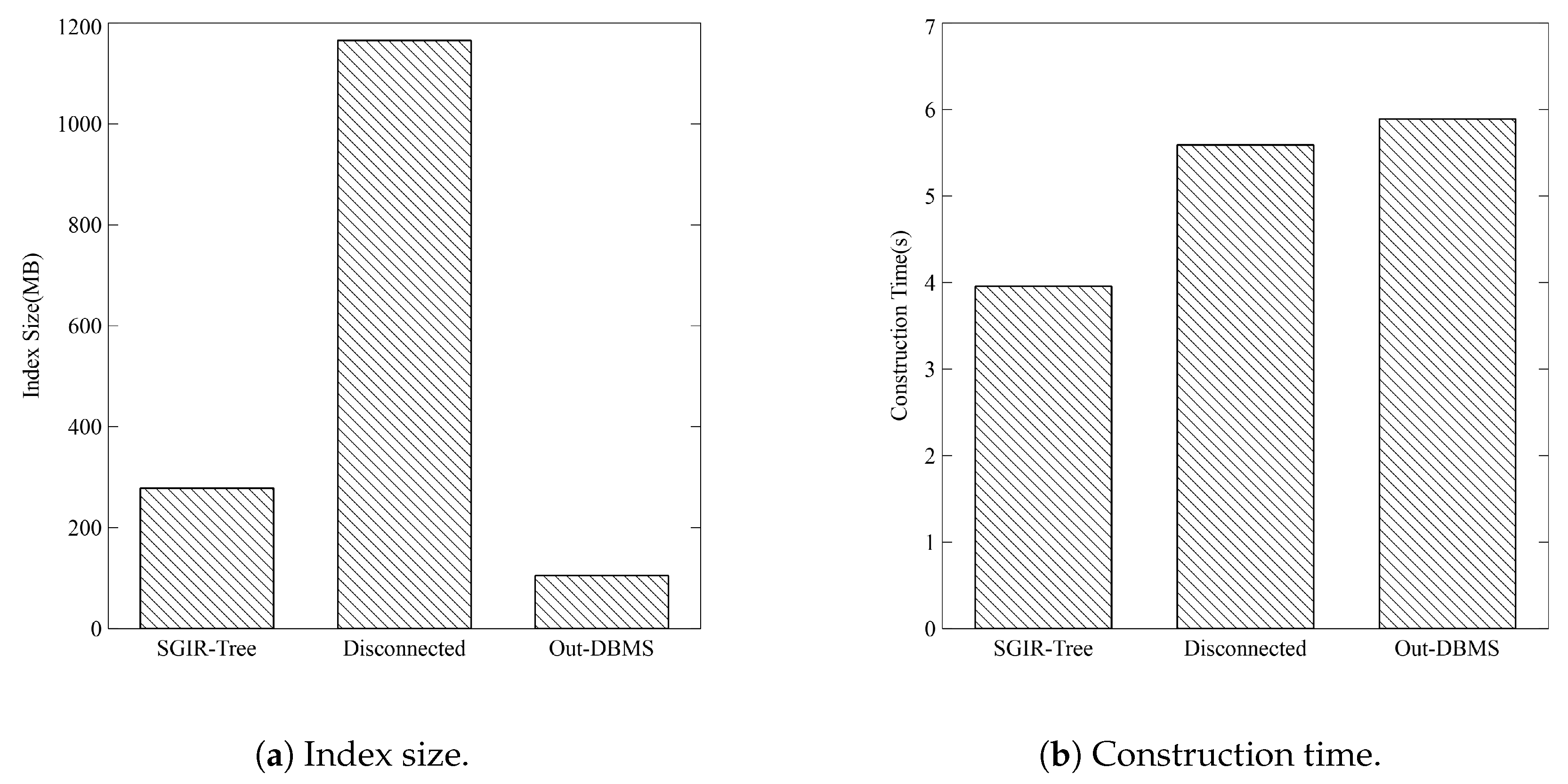
4.3. Index Overhead Results

The node capacity, a key parameter of the R-Tree, is set to the default value of 10. The comparison results of the index size and construction time of the SGIR-Tree, the disconnected index(Disconnected), and the Out-DBMS index are illustrated in Figure 3.

Figure 3a illustrates the comparison of index sizes among the three indices. The index size of the SGIR-Tree is approximately 278 MB, which is 4.2 times smaller than the disconnected index (approximately 1166 MB) and 2.8 times larger than the Out-DBMS index (approximately 105 MB). The proposed method is stored in an LPG, unlike the traditional R-Tree form like STR-TREE, which only stores the MBR and pointers to children. Therefore, each node not only stores the MBR and pointers to edges but also includes labels, which improves query efficiency by enabling faster node identification. Additionally, edges store pointers to connected nodes, labels, and MBRs; then, the MBR is also stored in the edges between leaf nodes and spatial nodes. This additional MBR storage allows for more precise spatial queries and reduces unnecessary node traversal, leading to a larger index size. The disconnected index has a very large index size because it duplicates the spatial nodes within the GDBMS to build the index. As illustrated in Figure 3b, the construction time of the proposed method is about 4 s, which is 1.4 times faster than the disconnected index (approximately 5.6 s) and 1.5 times faster than the Out-DBMS index (approximately 5.9 s). Despite the larger index size, the SGIR-Tree achieves faster construction times due to the efficient integration within the DBMS, which allows for direct access to data without the overhead of copying spatial nodes as in the disconnected index. Furthermore, being an In-DBMS approach, the SGIR-Tree avoids the overhead associated with loading and synchronizing an external index as required by the Out-DBMS STR-TREE method. This direct integration and optimized in-memory processing contribute to the faster construction times of the SGIR-Tree.

These results demonstrate that the proposed SGIR-Tree excels in terms of storage efficiency and construction speed. It significantly outperforms the disconnected spatial index stored within the GDBMS and also shows superior construction speed compared to the external STR-TREE from the JTS library; this suggests that the proposed method is an efficient indexing structure tailored to the characteristics of GDBMSs.

4.4. Query Overhead Results

In this subsection, we evaluate the query execution performance of the SGIR-Tree. We analyze its efficiency for various spatial query types and compare it with existing methods.

4.4.1. Query Overhead in SGIR-Tree

Spatial Join: The join operation used in this study is based on the spatial relations between geometric objects as defined by Egenhofer DE-9IM. The operation uses two spatial sets: Building and Highway sets, and Place and LandUse sets. These sets are chosen because Building and Highway have the highest number of spatial nodes, and Place and LandUse provide additional variety for evaluating the joins. As introduced earlier, spatial join operations using R-Trees involve comparing the MBR overlaps between nodes of different spatial sets. However, for the disjoint operation, it is impossible to perform calculations based on MBR overlaps of the R-Tree. Instead, we utilize the characteristic that the disjoint operation is the opposite of the intersects operation, calculating it as the remaining set after subtracting the results of the intersects operation from the total sets. Performing the disjoint operation between the Highway and Building spatial sets is not feasible due to the high memory load caused by this algorithm. Therefore, we additionally conduct join experiments between the spatial sets of Place and LandUse. Specifically, Place includes features such as neighborhoods, public squares, and cities, whereas LandUse encompasses areas such as greenfields, farmlands, and industrial areas.

Figure 4 illustrates the execution time and memory usage of the spatial join queries. Figure 4a,b represent the query times for Highway and Building, and Place and LandUse datasets, respectively, while Figure 4c,d show the memory overhead for these queries. First, examining the results for the Highway and Building dataset, the ‘intersects’ and ‘touches’ operations consume the most resources in terms of query execution time and memory usage. In particular, the ‘intersects’ operation has a memory usage of 6.5 MB, which is more than three times higher than the other operations, indicating that it has the most candidate spatial nodes. Conversely, the remaining operations exhibit relatively fast execution times and lower memory usage.

For the Place and LandUse dataset, the ‘disjoint’ operation has the longest execution time of approximately 8 s and the highest memory usage at 2630 MB; this is because the ‘disjoint’ operation is implemented by calculating all ‘intersects’ results and then excluding them from the total. In the Place and LandUse dataset, the ‘coveredBy’, ‘equals’, and ‘within’ operations show significantly faster execution times compared to other operations, which is likely due to the fewer number of node pairs satisfying these relationships. Overall, the proposed index structure effectively supports various spatial join operations and demonstrates stable performance even with large datasets.

KNN: The KNN queries are conducted on all spatial sets (Building, Highway, LandUse, Natural, Place, and Shop), varying the value of K as 1, 5, 25, and 125. Figure 5 shows the execution time and memory usage of the KNN queries.

Figure 5a,b show the KNN query performance of the SGIR-Tree as the value of K changes. The query execution time increases linearly as the value of K increases, while the memory usage exhibits a non-linear and fluctuating pattern. These patterns reflect the efficient structure and algorithmic characteristics of the SGIR-Tree. The execution time increases from 0.932 s at K = 1 to 1.217 s at K = 125, representing an approximately 1.31 times increase; this indicates that despite the 125-fold increase in the value of K, the execution time rises relatively gradually. In contrast, memory usage exhibits a more intriguing pattern. It decreases from 2.05 MB at K = 1 to 1.85 MB at K = 5. Thereafter, it increases to 2.42 MB at K = 25 and decreases again to 2.17 MB at K = 125. Comparing the memory usage at K = 5 (the lowest) and K = 25 (the highest) reveals a difference of only about 1.31 times. For K = 1 and K = 125, despite the 125-fold increase in the value of K, the memory usage increases by only 1.06 times. This memory usage pattern demonstrates the effective pruning capability of the SGIR-Tree. As explained in the Methodology section, the temporary distance used for pruning can increase as the value of K increases. With larger K values, more nodes are visited. Simultaneously, the larger temporary distance facilitates more pruning opportunities; this can result in an overall reduction in memory usage.

In summary, the execution time increases by 1.31 times, and the memory usage increases by a maximum of 1.31 times and a minimum of 1.06 times; this indicates that the SGIR-Tree can maintain both query performance and memory efficiency with large K values. Leveraging the structural advantages of the R-Tree and optimized algorithms tailored to graph databases, the SGIR-Tree is expected to offer high scalability and efficiency across various K values in practical applications for processing KNN queries.

Spatial Range: The spatial range queries are conducted on all spatial sets, varying the selectivity of the query range as 0.0001, 0.001, 0.01, and 0.1. As this selectivity is a parameter of the query point’s buffer, a larger value results in a wider range for the query MBR, leading to longer query times and higher memory overhead. Figure 6 illustrates the different selectivity ranges used in the experiment (Figure 6a), along with the execution time (Figure 6b) and memory usage (Figure 6c) of the spatial range queries.

The experimental results exhibit a general trend of increasing execution time and memory usage as the query range is increased. At the smallest range of 0.0001, the SGIR-Tree operates efficiently, with the lowest execution time and memory usage. As the range is increased to 0.001 and 0.01, performance changes are gradual; however, the index remains effective, maintaining execution times within 1 s and memory usage at approximately 2 MB. Visualizing the changes in query range (Figure 6a), it becomes evident that the buffer area grows by the square of the buffer distance as it increases from the Empire State Building; this is owing to the area of a circular buffer being proportional to the square of its radius. The largest query range of 0.1 covers most of New York City, resulting in a significant increase in memory usage to approximately 40 MB but still completes the query in approximately 4.8 s; this demonstrates that the SGIR-Tree functions effectively even when processing all spatial nodes in a wide area of the database.

Overall, the SGIR-Tree performs effectively across various query ranges, showing particularly high efficiency for small-range area queries. While it maintains good performance for large-range area queries, real-world applications can further optimize performance by appropriately adjusting query ranges or dividing large-range queries.

4.4.2. Comparison to Disconnected and Out-DBMS Spatial Index

Comparison to disconnected spatial index: Figure 7 present the performance comparison between the SGIR-Tree and the disconnected spatial index. This comparison is conducted using the spatial graph query $Q_{SG}=\langle S{P}_q,G_q\rangle$ as defined in Definition 4. The $S{P}_q$ component is executed using the parameters with the highest overhead from the previous experiments on spatial join, KNN, and spatial range queries, specifically, intersects, k = 125, and selectivity = 0.1. For the $G_q$ component, the condition is chosen to produce the most results during graph traversal after the spatial query: finding the color “beige” connected by the “HAS_COLOR” relationship to the Building nodes. The performance comparison metrics are the query execution time and memory overhead, excluding the $S{P}_q$ component. For both the SGIR-Tree and the disconnected spatial index, the process is the same up to $S{P}_q$. However, the disconnected spatial index requires additional matching between the $S{P}_q$ result nodes and the graph nodes for $G_q$ execution, whereas the SGIR-Tree integrates $S{P}_q$ and $G_q$, eliminating this additional matching process. Therefore, the comparison of the two indices is focused on the memory usage during the execution process after $S{P}_q$.

The results of $Q_{SG}$ with spatial join are shown in Figure 7a. The query time for the SGIR-Tree is approximately 90 s, which is approximately 4 s faster than that of 94 s for the disconnected index (improvement of approximately 1.04 times). In terms of memory usage, the SGIR-Tree uses approximately 0.0027 MB, whereas the disconnected index uses about 0.0207 MB, thereby indicating a difference of approximately eight times. In $Q_{SG}$ with the KNN (Figure 7b), the query time for the SGIR-Tree is 0.826 s, slightly higher than the 0.804 s of that of the disconnected index. However, there is a significant difference in memory usage. The SGIR-Tree uses 0.0008 MB, whereas the disconnected index uses 0.0133 MB. Thus, the SGIR-Tree consumes approximately 17 times less memory. For $Q_{SG}$ with the spatial range (Figure 7c), the query time for the SGIR-Tree is 2.991 s, approximately 1.4 s faster than the 4.362 s required by the disconnected index. There is a large difference in memory usage, with the SGIR-Tree using 0.00031 MB compared to 12.0007 MB for that of the disconnected index; this can be interpreted as the high selectivity of 0.1, including almost all spatial nodes, leading to significant memory overhead during matching in the disconnected index.

Overall, the SGIR-Tree shows improved performance compared to the disconnected spatial index for most types of queries. The significant improvement in memory usage is particularly notable because the SGIR-Tree structure directly connects the spatial index with the spatial nodes in the entire graph. This direct connection allows the results of $S_q$ to be immediately utilized in $G_q$, thereby eliminating the additional matching overhead required by the disconnected index.

Comparison to Out-DBMS spatial index: The STR-TREE supported by JTS does not handle spatial join and KNN queries; thus, only $G_S$ with spatial range queries are compared. The $S_q$ component targets the entire spatial sets with a selectivity of 0.1, and $G_q$ follows the same criteria as those in the disconnected spatial index experiments. As it is not possible to accurately measure the memory usage of the STR-TREE, only the query time is used as a metric. The comparison results are illustrated in Figure 8.

The average query time for the SGIR-Tree is 3.201 s, which is 73.631 s faster than the 76.832 s for the Out-DBMS index, representing a performance improvement of approximately 24 times. This significant difference can be attributed to the subgraph structure, which allows the spatial index to be directly utilized within the GDBMS, thereby reducing the data loading overhead associated with external indices. Specifically, STR-TREE requires approximately 70 s to only load the indices for all spatial sets. These results demonstrate that the SGIR-Tree offers advantages in query performance compared to the Out-DBMS spatial index approach. The SGIR-Tree is particularly effective when spatial and graph queries need to be processed together within the GDBMS environment. However, further research is needed to determine if these performance improvements hold in all scenarios. For example, it is necessary to analyze performance variations based on factors such as data scale, distribution, and query complexity.

5. Conclusions

This study proposes the SGIR-Tree for efficient spatial data management and query processing in GDBMSs. This method organically integrates the hierarchical structure of the R-Tree with the graph structure of the GDBMS, combining the efficiency of spatial indexing with the flexibility of graph databases. The core of the proposed method involves converting and storing the nodes and pointers of the R-Tree as nodes and edges in the GDBMS. Directly connecting leaf nodes with spatial entities enhances the connectivity between the index and the data, enabling the seamless integration of spatial searches and graph traversals. Furthermore, storing MBR information as properties of nodes and edges facilitates efficient filtering using the graph structure during spatial query processing. The experimental results clearly demonstrate the superiority of the proposed method. It exhibits significant improvements in execution time and memory usage compared to the disconnected spatial index and Out-DBMS spatial index in spatial graph queries with spatial join, KNN, and spatial range. The method maintains stable performance even with large datasets, thereby proving its applicability in real-world scenarios. This improvement is attributable to the effective integration of spatial data and graph structures by the SGIR-Tree structure, thus minimizing redundancy and enhancing search efficiency.

One major limitation of this study is that the dataset used is limited to a 1-hop structure, which does not fully reflect performance in real-world datasets with more complex relationships. Future research should further validate the proposed method using datasets with more complex relationships and various hop counts. In addition, implementing and optimizing the index in distributed environments could be an important research topic. Further research on adjusting and extending the proposed index structure for distributed systems is needed to handle large-scale spatial graph data efficiently.

In conclusion, the SGIR-Tree proposed in this study significantly improves the efficiency of spatial query processing in GDBMSs. This advancement is expected to provide a foundation for effectively utilizing spatial and graph data in various fields, such as location-based services, social network analysis, urban planning, and geographic information systems. The results of this study represent a milestone in the development of spatial data processing technologies in GDBMSs. The SGIR-Tree can evolve into a powerful tool to meet the complex spatial graph analysis needs in the era of big data by addressing its limitations and expanding its application range through future research.

References

1. Yeung, A.K.W.; Hall, G.B. Spatial Database Systems: Design, Implementation and Project Management; Springer Science & Business Media: Berlin/Heidelberg, Germany, 2007. [Google Scholar]
2. Sun, L.; Jin, B. Improving NoSQL Spatial-Query Processing with Server-Side In-Memory R*-Tree Indexes for Spatial Vector Data. Sustainability 2023, 15, 2442. [Google Scholar] [CrossRef]
3. Park, S.; Cheng, T. Framework for Constructing Multimodal Transport Networks and Routing Using a Graph Database: A Case Study in London. Trans. GIS 2023, 27, 1391–1417. [Google Scholar] [CrossRef]
4. Xiao, F.; Guo, W.; Liu, W.; Zeng, J. A Spatio-temporal Big Data Decision Support System of Real Estate. In Proceedings of the 2021 International Conference on Information Technology and Biomedical Engineering (ICITBE), Nanchang, China, 24–26 December 2021; pp. 30–34. [Google Scholar] [CrossRef]
5. Stadler, C.; Lehmann, J.; Höffner, K.; Auer, S. LinkedGeoData: A Core for a Web of Spatial Open Data. Semant. Web 2012, 3, 333–354. [Google Scholar] [CrossRef]
6. Qiao, Y.; Luo, X.; Li, C.; Tian, H.; Ma, J. Heterogeneous Graph-Based Joint Representation Learning for Users and POIs in Location-Based Social Network. Inf. Process. Manag. 2020, 57, 102151. [Google Scholar] [CrossRef]
7. Yue, P.; Tan, Z. 1.06 GIS Databases and NoSQL Databases. In Comprehensive Geographic Information Systems; Huang, B., Ed.; Elsevier: Oxford, UK, 2018; pp. 50–79. [Google Scholar] [CrossRef]
8. Sun, Y.; Sarwat, M. Riso-Tree: An Efficient and Scalable Index for Spatial Entities in Graph Database Management Systems. ACM Trans. Spat. Algorithms Syst. 2021, 7, 1–39. [Google Scholar] [CrossRef]
9. Li, W.; Wang, S.; Wu, S.; Gu, Z.; Tian, Y. Performance benchmark on semantic web repositories for spatially explicit knowledge graph applications. Comput. Environ. Urban Syst. 2022, 98, 101884. [Google Scholar] [CrossRef]
10. Bertella, P.G.K.; Lopes, Y.K.; de Oliveira, R.A.P.; Carniel, A.C. A Systematic Review of Spatial Approximations in Spatial Database Systems. J. Inf. Data Manag. 2022, 13, 2519. [Google Scholar] [CrossRef]
11. Sun, Y.; Sarwat, M. A Spatially-Pruned Vertex Expansion Operator in the Neo4j Graph Database System. GeoInformatica 2019, 23, 397–423. [Google Scholar] [CrossRef]
12. Guttman, A. R-Trees: A Dynamic Index Structure for Spatial Searching. In Proceedings of the 1984 ACM SIGMOD International Conference on Management of Data-SIGMOD ’84, Boston, MA, USA, 18–21 June 1984; p. 47. [Google Scholar] [CrossRef]
13. Bentley, J.L. Multidimensional Binary Search Trees Used for Associative Searching. Commun. ACM 1975, 18, 509–517. [Google Scholar] [CrossRef]
14. Sellis, T.K.; Roussopoulos, N.; Faloutsos, C. The R+-Tree: A Dynamic Index for Multi-Dimensional Objects. In Proceedings of the 13th International Conference on Very Large Data Bases, San Francisco, CA, USA, 1–4 September 1987; VLDB’87. pp. 507–518. [Google Scholar]
15. Beckmann, N.; Kriegel, H.P.; Schneider, R.; Seeger, B. The R*-Tree: An Efficient and Robust Access Method for Points and Rectangles. In Proceedings of the 1990 ACM SIGMOD International Conference on Management of Data, Atlantic City, NJ, USA, 23–26 May 1990; SIGMOD’90. pp. 322–331. [Google Scholar] [CrossRef]
16. Robinson, J.T. The K-D-B-tree: A Search Structure for Large Multidimensional Dynamic Indexes. In Proceedings of the 1981 ACM SIGMOD International Conference on Management of Data, Ann Arbor, MI, USA, 29 April–1 May 1981; SIGMOD’81. pp. 10–18. [Google Scholar] [CrossRef]
17. Procopiuc, O.; Agarwal, P.K.; Arge, L.; Vitter, J.S. Bkd-Tree: A Dynamic Scalable kd-Tree. In Advances in Spatial and Temporal Databases, Proceedings of the 8th International Symposium, SSTD 2003, Santorini Island, Greece, 24–27 July 2003; Springer: Berlin/Heidelberg, Germany, 2003; pp. 46–65. [Google Scholar] [CrossRef]
18. Finkel, R.A.; Bentley, J.L. Quad Trees a Data Structure for Retrieval on Composite Keys. Acta Inform. 1974, 4, 1–9. [Google Scholar] [CrossRef]
19. Amiri, A.M.; Samavati, F.; Peterson, P. Categorization and Conversions for Indexing Methods of Discrete Global Grid Systems. ISPRS Int. J. Geo-Inf. 2015, 4, 320–336. [Google Scholar] [CrossRef]
20. Zhu, J.; Chong, H.Y.; Zhao, H.; Wu, J.; Tan, Y.; Xu, H. The Application of Graph in BIM/GIS Integration. Buildings 2022, 12, 2162. [Google Scholar] [CrossRef]
21. Brodt, A.; Nicklas, D.; Mitschang, B. Deep Integration of Spatial Query Processing into Native RDF Triple Stores. In Proceedings of the 18th SIGSPATIAL International Conference on Advances in Geographic Information Systems, San Jose, CA, USA, 2–5 November 2010; GIS’10. pp. 33–42. [Google Scholar] [CrossRef]
22. Wang, D.; Zou, L.; Feng, Y.; Shen, X.; Tian, J.; Zhao, D. S-Store: An Engine for Large RDF Graph Integrating Spatial Information. In Database Systems for Advanced Applications, Proceedings of the 18th International Conference, DASFAA 2013, Wuhan, China, 22–25 April 2013; Meng, W., Feng, L., Bressan, S., Winiwarter, W., Song, W., Eds.; Springer: Berlin/Heidelberg, Germany, 2013; pp. 31–47. [Google Scholar] [CrossRef]
23. Liagouris, J.; Mamoulis, N.; Bouros, P.; Terrovitis, M. An Effective Encoding Scheme for Spatial RDF Data. Proc. VLDB Endow. 2014, 7, 1271–1282. [Google Scholar] [CrossRef]
24. Theocharidis, K.; Liagouris, J.; Mamoulis, N.; Bouros, P.; Terrovitis, M. SRX: Efficient Management of Spatial RDF Data. VLDB J. 2019, 28, 703–733. [Google Scholar] [CrossRef]
25. Shi, J.; Wu, D.; Mamoulis, N. Top-k Relevant Semantic Place Retrieval on Spatial RDF Data. In Proceedings of the 2016 International Conference on Management of Data, San Francisco, CA, USA, 26 June–1 July 2016; SIGMOD’16. pp. 1977–1990. [Google Scholar] [CrossRef]
26. Cai, Z.; Kalamatianos, G.; Fakas, G.J.; Mamoulis, N.; Papadias, D. Diversified Spatial Keyword Search on RDF Data. VLDB J. 2020, 29, 1171–1189. [Google Scholar] [CrossRef]
27. Virtuoso Documentation. Available online: https://docs.openlinksw.com/virtuoso/sqlrefgeospatial/ (accessed on 24 September 2024).
28. Osman, T. GeoSPARQL-Jena: Implementation and Benchmarking of a GeoSPARQL Graphstore. Eur. Conf. Knowl. Manag. 2022, 23, 885–894. [Google Scholar] [CrossRef]
29. Jin, X.; Shin, S.; Jo, E.; Lee, K.H. Collective Keyword Query on a Spatial Knowledge Base. IEEE Trans. Knowl. Data Eng. 2019, 31, 2051–2062. [Google Scholar] [CrossRef]
30. Wu, D.; Hou, C.; Xiao, E.; Jensen, C.S. Semantic Region Retrieval from Spatial RDF Data. In Proceedings of the Database Systems for Advanced Applications; Nah, Y., Cui, B., Lee, S.W., Yu, J.X., Moon, Y.S., Whang, S.E., Eds.; Springer: Cham, Switzerland, 2020; pp. 415–431. [Google Scholar] [CrossRef]
31. Wang, C.J.; Ku, W.S.; Chen, H. Geo-Store: A spatially-augmented SPARQL query evaluation system. In Proceedings of the 20th International Conference on Advances in Geographic Information Systems, Redondo Beach, CA, USA, 6–9 November 2012; SIGSPATIAL’12. pp. 562–565. [Google Scholar] [CrossRef]
32. Lee, K.; Liu, L.; Ganti, R.K.; Srivatsa, M.; Zhang, Q.; Zhou, Y.; Wang, Q. Lightweight Indexing and Querying Services for Big Spatial Data. IEEE Trans. Serv. Comput. 2016, 12, 343–355. [Google Scholar] [CrossRef]
33. Leeka, J.; Bedathur, S.; Bera, D.; Lakshminarasimhan, S. STREAK: An Efficient Engine for Processing Top-k SPARQL Queries with Spatial Filters. arXiv 2017, arXiv:1710.07411. [Google Scholar]
34. RDF4j Github Repository. Available online: https://github.com/eclipse-rdf4j/rdf4j/issues/1160 (accessed on 24 September 2024).
35. Stardog Documentation Release-Note. Available online: https://docs.stardog.com/release-notes/stardog-platform (accessed on 24 September 2024).
36. GraphDB 7.0 Documnetation. Available online: https://graphdb.ontotext.com/documentation/7.0/enterprise/geo-spatial-extensions.html?highlight=spatial%20index# (accessed on 24 September 2024).
37. Hadjieleftheriou, M.; Hoel, E.; Tsotras, V.J. SaIL: A Spatial Index Library for Efficient Application Integration. GeoInformatica 2005, 9, 367–389. [Google Scholar] [CrossRef]
38. Huang, W.; Raza, S.A.; Mirzov, O.; Harrie, L. Assessment and Benchmarking of Spatially Enabled RDF Stores for the Next Generation of Spatial Data Infrastructure. ISPRS Int. J. Geo-Inf. 2019, 8, 310. [Google Scholar] [CrossRef]
39. Neo4j Spatial Plugin Github Repository. Available online: https://github.com/neo4j-contrib/spatial (accessed on 24 September 2024).
40. JanusGraph Github Repository. Available online: https://github.com/JanusGraph/janusgraph/issues/3015 (accessed on 24 September 2024).
41. JanusGraph Github Repository. Available online: https://github.com/JanusGraph/janusgraph/commits/master/janusgraph-lucene/src/main/java/org/janusgraph/diskstorage/lucene/LuceneIndex.java?after=4a576f67ff0e53b699ed078dad964d448bc94b10+34 (accessed on 24 September 2024).
42. NebulaGraph Documentation. Available online: https://www.nebula-graph.io/posts/explore-geospatial-data-with-nebulagraph (accessed on 24 September 2024).
43. TigerGraph Blog. Available online: https://medium.com/tigergraph/leveraging-geospatial-data-with-a-native-parallel-graph-database-d2c92e24d675 (accessed on 24 September 2024).
44. Kamel, I.; Faloutsos, C. Hilbert R-tree: An Improved R-tree Using Fractals. In Proceedings of the 20th International Conference on Very Large Data Bases, San Francisco, CA, USA, 12–15 September 1994; VLDB’94. pp. 500–509. [Google Scholar]
45. Roumelis, G.; Vassilakopoulos, M.; Loukopoulos, T.; Corral, A.; Manolopoulos, Y. The xBR+-Tree: An Efficient Access Method for Points. In Proceedings of the Database and Expert Systems Applications, Valencia, Spain, 31 August 2015; Chen, Q., Hameurlain, A., Toumani, F., Wagner, R., Decker, H., Eds.; Springer: Cham, Switzerland, 2015; pp. 43–58. [Google Scholar] [CrossRef]
46. Gu, T.; Feng, K.; Cong, G.; Long, C.; Wang, Z.; Wang, S. The RLR-Tree: A Reinforcement Learning Based R-Tree for Spatial Data. Proc. ACM Manag. Data 2023, 1, 63:1–63:26. [Google Scholar] [CrossRef]
47. Lee, T.; Moon, B.; Lee, S. Bulk Insertion for R-Tree by Seeded Clustering. In Database and Expert Systems Applications, Proceedings of the 14th International Conference, DEXA 2003, Prague, Czech Republic, 1–5 September 2003; Springer: Berlin/Heidelberg, Germany, 2003; pp. 129–138. [Google Scholar] [CrossRef]
48. Cheung, K.L.; Fu, A.W.C. Enhanced Nearest Neighbour Search on the R-tree. ACM SIGMOD Rec. 1998, 27, 16–21. [Google Scholar] [CrossRef]
49. Brinkhoff, T.; Kriegel, H.P.; Seeger, B. Efficient Processing of Spatial Joins Using R-trees. ACM SIGMOD Rec. 1993, 22, 237–246. [Google Scholar] [CrossRef]
50. Dsouza, A.; Tempelmeier, N.; Gottschalk, S.; Yu, R.; Demidova, E. WorldKG: World-Scale Completion of Geographic Information. In Volunteered Geographic Information: Interpretation, Visualization and Social Context; Burghardt, D., Demidova, E., Keim, D.A., Eds.; Springer Nature: Cham, Switzerland, 2023; pp. 3–19. [Google Scholar] [CrossRef]
51. Yang, J.; Jang, H.; Yu, K. Geographic Knowledge Base Question Answering over OpenStreetMap. ISPRS Int. J. Geo-Inf. 2024, 13, 10. [Google Scholar] [CrossRef]
52. Hoffart, J.; Suchanek, F.M.; Berberich, K.; Weikum, G. YAGO2: A Spatially and Temporally Enhanced Knowledge Base from Wikipedia. Artif. Intell. 2013, 194, 28–61. [Google Scholar] [CrossRef]
53. Karalis, N.; Mandilaras, G.; Koubarakis, M. Extending the YAGO2 Knowledge Graph with Precise Geospatial Knowledge. In The Semantic Web–ISWC 2019, Proceedings of the 18th International Semantic Web Conference, Auckland, New Zealand, 26–30 October 2019; Ghidini, C., Hartig, O., Maleshkova, M., Svátek, V., Cruz, I., Hogan, A., Song, J., Lefrançois, M., Gandon, F., Eds.; Springer: Cham, Switzerland, 2019; pp. 181–197. [Google Scholar] [CrossRef]
54. Bast, H.; Brosi, P.; Kalmbach, J.; Lehmann, A. An Efficient RDF Converter and SPARQL Endpoint for the Complete OpenStreetMap Data. In Proceedings of the 29th International Conference on Advances in Geographic Information Systems, Beijing, China, 2–5 November 2021; SIGSPATIAL’21. pp. 536–539. [Google Scholar] [CrossRef]
Figure 1. Comparison of isolated and subgraph spatial index approaches in a social network graph with R-Tree index. (a) Isolated index: Spatial entities within 500 m can be found (green map marker), but matching with the entire graph is required. (b) Subgraph index: Restaurants within 500 m can be directly identified and graph traversal used to find specific restaurants visited by connected users. The two orange boxes inside the leaf node indicate the Minimum Bounding Rectangles (MBRs) for Bonchon and the adjacent spatial node.
Ijgi 13 00346 g001
Figure 2. Example of the structure in the proposed SGIR-Tree.
Ijgi 13 00346 g002
Figure 3. Indices overhead.
Ijgi 13 00346 g003
Figure 4. Spatial join query overhead.
Ijgi 13 00346 g004
Figure 5. KNN query overhead.
Ijgi 13 00346 g005
Figure 6. Spatial Range Query.
Ijgi 13 00346 g006
Figure 7. Comparison of SGIR-Tree to disconnected index.
Ijgi 13 00346 g007
Figure 8. Comparison SGIR-Tree to Out-DBMS Index.
Ijgi 13 00346 g008