Abstract
Enriching and updating maps are among the most important tasks of any urban management organization for informed decision making. Urban cadastral map enrichment is a time-consuming and costly process, which needs an expert’s opinion for quality control. This research proposes a smart framework to enrich a cadastral base map using a more up-to-date map automatically by machine learning algorithms. The proposed framework has three main steps, including parcel matching, parcel change detection and base map enrichment. The matching step is performed by checking the center point of each parcel in the other map parcels. Support vector machine and random forest classification algorithms are used to detect the changed parcels in the base map. The proposed models employ the genetic algorithm for feature selection and grey wolf optimization and Harris hawks optimization for hyperparameter optimization to improve accuracy and performance. By assessing the accuracies of the models, the random forest model with feature selection and grey wolf optimization, with an F1-score of 0.9018, was selected for the parcel change detection method. Finally, the detected changed parcels in the base map are deleted and relocated automatically with corresponding parcels in the more up-to-date map by the affine transformation.
1. Introduction
Cities are becoming more complex day to day due to increments in population, urbanization and the pace of construction and change [1]. The vast extents, high densities and fast changes in cities and urban areas make measuring, managing, monitoring, mapping and modeling urban changes more challenging and time-consuming for organizations and researchers [1]. The growth of urbanization causes intensive use of land. The faster growth of the physical extent of urban areas compared to their population causes more land to be used for urban development [2]. Hence, efficient land administration and parcel-based land development modeling play an important role in sustainable urban growth [3,4]. Land Administration Systems (LASs) in cities are for intelligent land and urban space management [5]. Land information is required for different LAS components, which are land development, land use, land value and land tenure [5]. Urban cadastral maps as a part of land information are large-scale maps that contain dimensions, shapes, spatial relationships and different attributes of information about land parcels [6].
Enrichment of urban cadastral maps helps organizations to make accurate and timely decisions for urban management [7]. Urban cadastral map enrichment and checking for the accuracy and reliability of data are important duties of urban management organizations [8]. Urban cadastral maps are enriched with the help of legal documents for geometric changes, incorporating new information and data, or the removal of inaccurate data [8]. Enrichment and updating of urban cadastral maps are as important as their production and pose different challenges [9]. Map enrichment is a parcel-based time-consuming process due to the large number of parcels and the large amount of information in urban areas and needs visual parcel-to-parcel checking and a high level of expertise in the different steps of enrichment, including matching, change detection and base map enrichment. Hence, detecting changes in a map with more up-to-date maps from other sources automatically by machine learning algorithms can reduce the time and cost of map enrichment. Machine learning methods such as random forest are good methods with computational advantages for large-scale urban cadastral maps and spatial data analyses [4]. Supervised machine learning methods are some of the change detection techniques that require training data for classification [10].
Map enrichment has been performed using different methods and data and for different usages. In some research, historical and analogue cadastral maps have been used to determine ownership boundaries and in the renewal of cadastral maps [6,9,11]. Data and map integration are other methods for map enrichment. Integration of different web maps [12] and enriching a base map with a more up-to-date map, aerial images, orthophotos and remote sensing (RS) imagery [7,13,14,15,16,17] are some of the spatial data fusion and integration methods which have been previously investigated.
Artificial intelligence methods, including machine learning and deep learning, have recently been used very much for map enrichment; updating; object, boundary and change detection; and spatial data fusion [14,15,18,19,20]. In [18], a combination of data-level fusion and feature-level fusion was employed for natural object detection by multi-source geospatial data and deep learning. Deep learning methods have been implemented to align and update cadaster maps with satellite images [19], detect visible land boundaries automatically with aerial images and revise existing cadastral maps [20]. In [21], a comparison between manual approaches and machine learning algorithms for extracting visible cadaster boundaries from satellite images in rural and urban areas was made, and the authors showed that machine learning algorithms have lower costs, require less time and achieve a higher accuracy than manual approaches.
Most previous research has been focused on aerial or satellite images to enrich base maps. Most of them have been employed in small areas, or map features have been enriched case by case, and less attention has been given to enriching base maps with more recent maps in a vector space in vast, dense and complex urban areas. In addition, automatic change detection and map modification with an acceptable accuracy have been less investigated. Hence, the contribution of this research is to propose an intelligent framework to enrich cadastral parcels in a base map of an urban area with a more up-to-date map automatically.
The remaining parts of this paper are as follows: Section 2 discusses the methodology of the research, the proposed methods and their evaluation. Section 3 presents the study area, the employed data and the implementation of the proposed method. Section 4 constitutes the discussion, and Section 5 concludes the paper and recommends some directions for future research.
2. Proposed Methodology
This research is aimed at reaching an intelligent framework for enriching land parcels in urban base maps. Two urban maps were employed in this research: a base map (a Cadaster Department map, a map at 1:2000 scale in the UTM (Zone 39N) projection system, produced in 2002) that was to be enriched and a more up-to-date urban map (a Tehran Municipality map, a map at 1:1000 scale in the UTM (Zone 39N) projection system, produced in 2014) that was used to enrich the base map. Parcels in each map were target features in this research, and the focus was only on enriching the geometry of the parcels. Due to limitations on data access, other information for each parcel, such as registration, legal and descriptive information, was not investigated. This framework has three main steps: matching, parcel change detection and base map enrichment. In this research, after preprocessing the data, including format and scale homogenization and topology checking, a matching algorithm was employed to find the corresponding parcels for each parcel in each of the maps. Then, 38 different geometric, topologic and statistical parameters were calculated for each parcel in each of the maps to be used in support vector machine (SVM) and random forest (RF) machine learning algorithms for detecting changes in the base map intelligently. There are different methods to increase the accuracy of models, including data addition, dimension reduction, regularization, missing value and outlier management, feature engineering, feature selection, ensemble learning, and hyperparameter optimization. Missing value and outlier management, feature engineering, feature selection, ensemble learning (using random forest algorithms), and hyperparameter optimization were employed in this research in the models’ training steps. In training the models, feature selection and hyperparameter optimization were used to increase the accuracy of change detection. Finally, the changed parcels that were detected in the previous step were replaced automatically by new parcels in the more up-to-date map. In this step, each parcel in the more up-to-date map that corresponds to a changed parcel in the base map is located on the base map by the unchanged neighbors of the parcel.
2.1. Matching
In spatial datasets, the matching process is the identification of corresponding features in two or more different datasets in the same spatial coverage, where the corresponding items represent the same feature in the real world [22]. Matching is one of the main steps in enriching and integrating heterogeneous spatial data, which is performed to add new data, maintain similar and unchanged spatial data, remove additional data, and reduce differences and contradictions between data and information in the datasets [23,24].
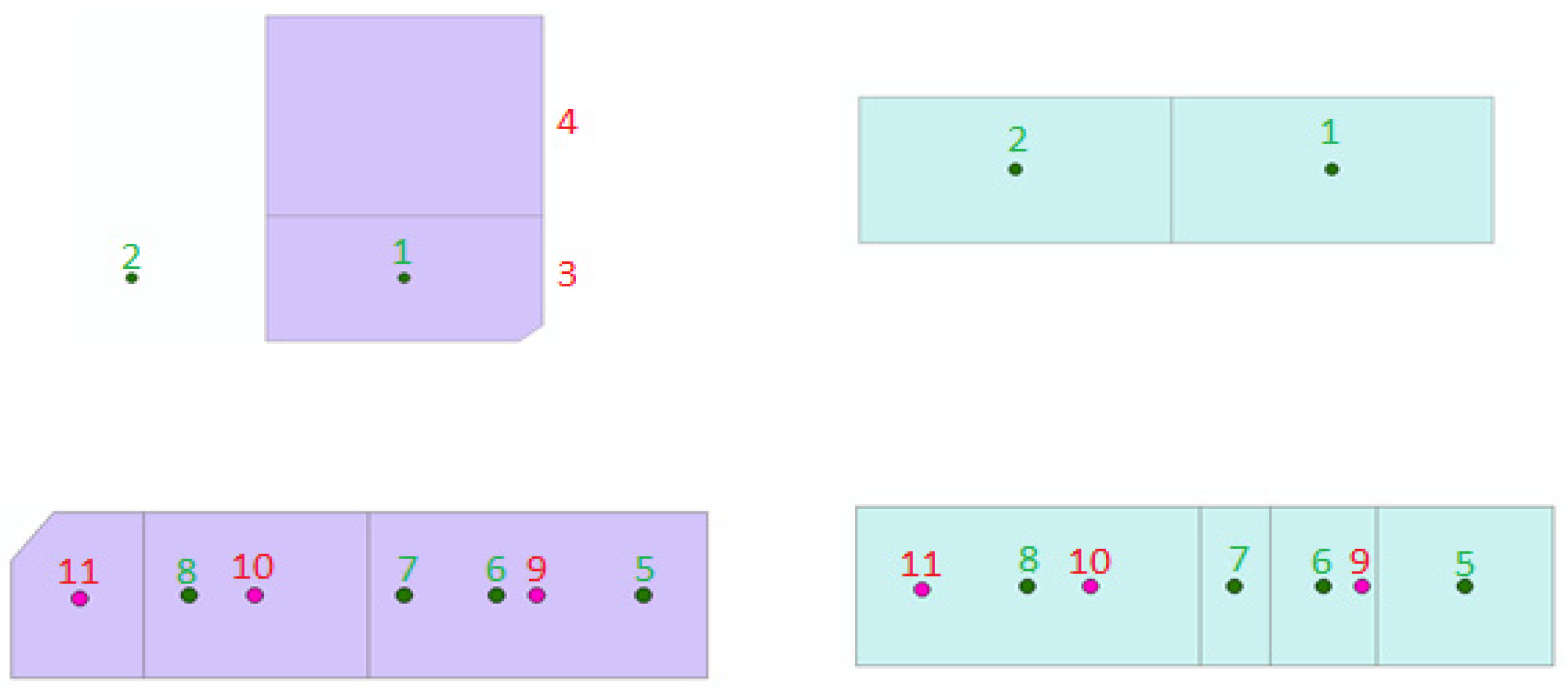
Since the data used in this research are parcels, if these parcels are used and the intersection or sharing of borders between parcels of the first map and the second map is examined, the neighbors of the parcels are also considered as the corresponding parcels. This causes errors in detecting corresponding parcels. Hence, to solve this problem, according to Figure 1, gravity centers of parcels are calculated and the matching process is performed by these gravity centers.
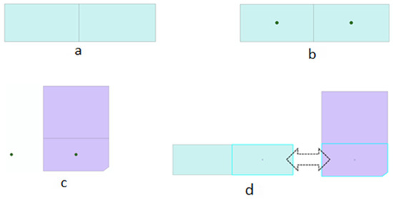
Figure 1.
Parcel matching. Green parcels: base map parcels, green points: gravity centers of base map parcels, purple parcels: second map parcels. (a) Base map parcels. (b) Calculated gravity centers of parcels. (c) Transfer of center points to second map. (d) Detection of the corresponding parcels.
The gravity center is the center of mass of a parcel that may fall inside or outside the parcel. The coordinate of the gravity center point () of a non-self-intersecting parcel is calculated by Equations (1) and (2) [25].
where (, ) is the coordinate of the vertex of the polygon, (, ) and (, ) are the same, and is the signed area of the polygon that is calculated by the Shoelace formula (Gauss’s area formula) by Equation (3) [25].
In this research, to identify the corresponding parcels in the base map and the second map, the gravity centers of the parcels in the base map were calculated. Then, parcels from the second map where these centers were located were considered as corresponding parcels for each parcel in the base map. In order to consider all the changes for the parcels in the base map compared to the more up-to-date map, this matching must be performed in both maps, which means that this matching should be implemented in parcels in the second maps too. Figure 2 illustrates the matching method in this research.
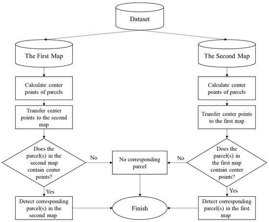
Figure 2.
Parcel matching process.
It is necessary to implement the matching algorithm in both maps to reach all these relations. Based on these relations, some changes in the base map can be detected. To better train and evaluate the change detection model, training and test data should be selected from all categories that exist in the matching process. Table 1 and Figure 3 show the different relations in the matching process.

Table 1.
Matching relations.

Figure 3.
Parcel matching. Green parcels: base map parcels, green points and numbers: gravity centers of base map parcels, purple parcels: second map parcels, red points and numbers: gravity centers of second map parcels.
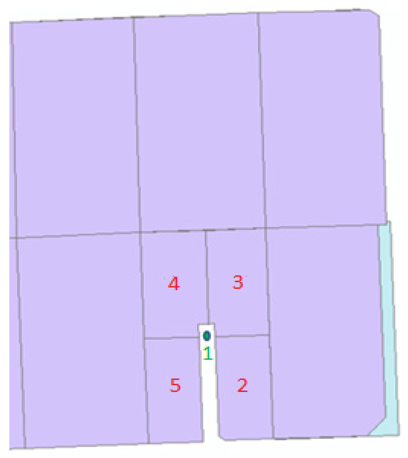
Because of the effect of the number of vertices of a polygon in determining the center of gravity of that polygon, the validation of matching is performed for parcels with different numbers of vertices. Figure 4 shows the effect of the number of vertices on determining the center of gravity and their effect on incorrect matching.
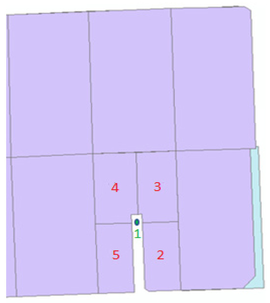
Figure 4.
Effect of number of vertices in determining the center of gravity. Green parcels: base map parcels, green points and numbers: gravity centers of base map parcels, purple parcels: second map parcels, red numbers: the second map parcels that corresponds to parcel number one from the base map.
In Figure 4, parcel number one corresponds to parcels number two, three, four and five, and it is the union of parcels in the second map, and its center of gravity is point number one, which is not located inside any parcels of the second map. If the matching is not performed from the second map to the first, this feature will not be correctly matched, or, if the parcel is not separated, the parcel will not be matched correctly.
2.2. Classification and Parcel Change Detection Modeling
The purpose of this step is to find parcels that have changed in the base map. For this purpose, after finding the corresponding parcels and by checking the geometric, topologic and statistical parameters, the changed parcels are identified by classification with support vectors machine (SVM) and random forest (RF) methods. To increase accuracy and reduce computational complexity, feature selection was used and hyperparameters were optimized by metaheuristic algorithms.
The geometric, topologic and statistical parameters are important parameters for features in maps. Hence, 38 different geometric, topologic and statistical parameters were considered for comparing parcels in the two maps [26,27]. To check the correlation between the parameters and features and prevent noise in the models, a correlation matrix was calculated between the calculated parameters (features) and then the parameters were selected for modeling. By checking the correlation of features, 19 dependent features were removed from the list of features of the parcels, and a total of 19 features with low dependencies were considered for each parcel to be used in the modeling. Table 2 shows a list of all the geometric, topologic and statistical parameters considered and the ones that were selected after checking the correlation of the features.

Table 2.
Geometric, topologic and statistical parameters and the ones that were selected after the correlation checking of the features.
2.2.1. Support Vector Machine
The support vector machine (SVM) is an algorithm that searches for an optimum hyperplane for linear separation of categories by mapping the training data in a non-linear way to a higher dimension [28]. This algorithm uses support vectors and edges to find this hyperplane. The advantages of this algorithm are its ability to model linear, non-linear and complex problems, its high accuracy, and its low probability of data overfitting. This algorithm is suitable for classification and numerical predictions [28,29,30]. If the data are located above the separating hyperplane, they are labeled 1; otherwise, they are labeled −1. The hyperplane equation corresponds to Equation (4) [31].
where is the normal vector that is perpendicular to the hyperplane, is a deviation number and (an error margin parameter) specifies the extent of violation of the determined boundary for each data. is used to prevent the adverse effect of noise data on decision-making boundaries and overfitting. Equation (5) is for optimization, and the new data are classified by a trained SVM and the Lagrange formulation according to Equation (6) [31].
In Equation (5), is the variable that regularizes the allowable value of the model for misclassification [31]. In Equation (6), is the label of the class for and is a new data. The Lagrangian coefficients and are numerical parameters from the optimization in Equation (5) [31].
2.2.2. Random Forest
There are various methods to improve performance and classification accuracy. The ensemble learning method is one of these methods, and the desired model consists of several classifiers. There is a high possibility of error if basic classifiers are used, but in ensemble methods, if more than half of the categories are wrong, the final output will contain errors [31]. Boosting and bagging are some methods of ensemble learning methods [32]. In bagging algorithms, models are trained simultaneously, in parallel and independently. To create each model, data are randomly selected from the main dataset, while there will be a possibility of having some data in all or some models. Finally, the result will be equal to the vote of the majority of the models. One of the bagging algorithms is the random forest (RF) algorithm [31,32,33]. In the RF algorithm. the classifiers used in the ensemble method are of the decision tree algorithms, and, finally, the best class is predicted based on voting. This algorithm performs better in comparison with boosting algorithms and has better performance in datasets with errors or outliers [31,34].
2.2.3. Genetic Algorithm
The genetic algorithm (GA) is one of the evolutionary and meta-heuristic computing methods, which is based on Darwin’s theory of biological evolution [35]. This algorithm has been used in feature selection for parcel change detection. At first, an initial population that includes a set of random rules is created. Each rule in this algorithm is coded with the help of a K-bit chromosome, where K is the number of values in that rule. Then, a new population of meritorious rules is generated based on the theory of survival of the fittest. New generations and children are created by genetic operators, such as selection, intersection and mutation, from the appropriate rules. The process of producing new populations by the populations of the previous stage continues until the termination condition is fulfilled. This termination condition can be the fulfillment of the fitness threshold of each of the rules in the final population, the production of a certain number of new populations, or the creation of several populations without improving the rejection of the rules fitness [31,36,37].
2.2.4. Grey Wolf Optimization
Grey wolf optimization (GWO) is one of the meta-heuristic algorithms based on the collective intelligence and social behavior of grey wolves during hunting [38]. Due to the examination of the grey wolf algorithm with some other meta-heuristic algorithms and the presentation of competitive results, as well as proof of the application of the grey wolf algorithm for engineering problems with an unknown search space [38], this method was selected as one of the optimization algorithms in this research. The hunting process in grey wolves includes searching and identifying prey, surrounding the prey, and attacking the prey [38]. The wolves in each pack are divided into one of four kinds: Alpha, Beta, Delta and Omega. Optimization is performed by three wolves: Alpha, Beta and Delta. In the grey wolf optimization algorithm, Alpha is the best solution, and Beta and Delta are the second and third best solutions, respectively. Equations (7)–(10) present the grey wolf optimization algorithm [38].
where t is the iteration number, A and C are the coefficient vectors, is the prey location vector, X is the grey wolf location vector, and and are random vectors in the range from zero to one and decrease linearly from two to zero during iterations. The new positions of each wolf in the grey wolf algorithm are calculated based on the best positions, which are the positions of the Alpha, Beta and Delta wolves. Equations (11)–(13) present the update of these locations [38].
2.2.5. Harris Hawks Optimization
The Harris hawks optimization (HHO) algorithm is a population-based algorithm that is inspired by the chase behavior of Harris hawks in surprising their prey [39]. This algorithm has been used in this research due to the comparison of the Harris hawks optimization algorithm with other nature-inspired optimization algorithms in several engineering problems and the promising and sometimes competitive results of the Harris hawks optimization algorithm with respect to other meta-heuristic algorithms [39]. The Harris hawks algorithm has three main stages of exploration: transition from exploration to exploitation and exploitation (extraction). In the exploration phase, the location vectors of the hawks are calculated by Equations (14) and (15) [39].
where q ≥ 0.5 is for situations when the hawks are randomly located in trees and waiting for the prey and q < 0.5 is for cases when the hawks’ locations are based on other hawk’s locations. In addition, X(t + 1) is the location vector in the ith iteration, is the position of the prey, X(t) is the current location vector of the hawks, is the location of a random hawk in the current population, is the average location of the current population of hawks, and as well as q are random numbers between zero and one, which are changed and updated in each iteration. LB and UB represent the upper and lower bounds for the variables. N is the total number of hawks, and is the location of each hawk in the i iteration.
To transfer from the exploration stage to the exploitation (extraction) stage, it is necessary to calculate the energy of the prey. This energy is calculated by Equation (16) [39].
where E is the energy of the prey to escape, T is the maximum number of repetitions and is the initial energy of the prey. has a value between negative one and positive one which changes in each iteration. This energy decreases from one to negative one during the changes.
At the exploitation stage, Harris hawks have four methods of attacking prey based on their prey escape behavior and their pursuit method. These methods are soft besiege, hard besiege, soft besiege with progressive rapid dives, and hard besiege with progressive rapid dives [39]. The Equations (17) and (18) are related to soft besiege [39].
The values of ΔX(t) are the difference between the prey location and the current location in repetition t, , and is a random number between zero and one. The value of J represents the power of the prey’s random jump in all jumps. which changes randomly in each iteration.
The location of each hawk is updated by Equation (19) in hard besiege [39].
In the soft besiege with progressive rapid dives method, first, the hawks’ location and next movements are determined by Equation (20) and a soft besiege. Then, ac-cording to Equations (21) and (22), the hawks will dive towards the prey, and, finally, their locations in soft besiege are updated by Equation (23) [39].
where D is the dimension of the problem, S is a random vector with size 1*D and LF is the flight function calculated by Equation (22). U and v are random values between zero and one, and beta has a constant value of 1.5.
In hard besiege with progressive rapid dives, the locations of hawks in hard besiege are updated by Equation (23), with the difference that the Y and Z values are calculated by Equations (24) and (25) [39].
2.2.6. Validation
To validate the modeling and to calculate the accuracy of parcel change detection, the root mean square error (RMSE), overall accuracy (accuracy), precision, recall and F1-score were used in this research. According to Equation (26), the RMSE was used to calculate loss functions [40]. The confusion matrix is shown in Table 3 [41].

Table 3.
Confusion matrix.
According to the confusion matrix, accuracy, precision, recall and F1-score are calculated by Equations (27)–(30) [42].
Table 4 shows the confusion matrix for the parcel change detection modeling. This matrix indicates the identification of changes in parcels correctly or incorrectly [42].

Table 4.
Confusion matrix for parcel change detection modeling.
2.2.7. The Proposed Methodology
The proposed model contains SVM and RF classification integrated with the GA for feature selection and the GWO or HHO algorithms for hyperparameter optimization in each iteration of training the models to improve their accuracy.
2.3. Base Map Enrichment
After detecting the changed parcels in the base map, the process of automatic enrichment of the base map (the Cadaster Department map) was performed with the more up-to-date map (the Tehran Municipality map), as shown in Figure 5. First, the detected changed parcels were removed from the base map. In the second step, for each removed parcel in the base map, the nearest neighboring parcels with the corresponding parcel in the more up-to-date map were identified, and then, in the third step, the transformation parameters between the neighbors of that parcel were calculated from the most up-to-date map to the base map. Then, in the fourth step, the vertices of the desired parcel in the updated map were transferred to the base map by the calculated transformation parameters. Finally, in the fifth step, the base map was checked against topologic errors to evaluate the enrichment.
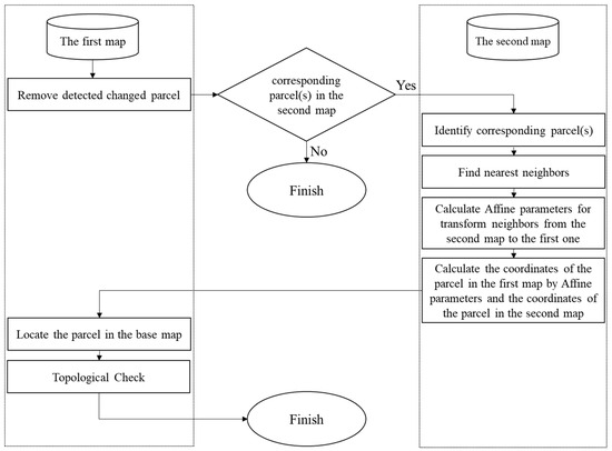
Figure 5.
Base map enrichment with the more up-to-date map.
The affine transformation was used in this research to transform between the maps and enrich the base map due to the two-dimensional maps and features [43]. Equations (31) and (32) show the affine transformation. The coordinates of the vertices of the parcels were used in the equations to find the parameters or the transferred coordinates.
where x and are the initial coordinates, are the transferred coordinates. and c and d are the transfer factors. a and b are calculated by Equations (33) and (34) [43].
where is the scale factor and alpha is the rotation angle, which are calculated from Equations (35) and (36) [43].
3. Implementation
3.1. Study Area
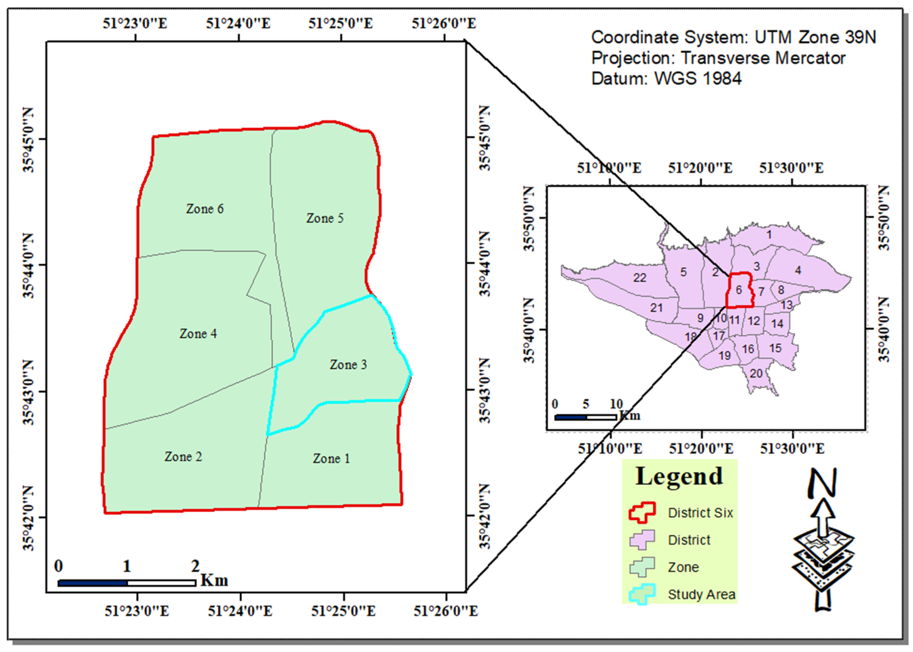
The study area is the third zone of Tehran Municipality District Six. The capital of Iran, Tehran, consists of 22 districts, 125 zones and 355 neighborhoods. District Six is one of the oldest districts of Tehran Municipality, which is geographically located in the center of Tehran. This district has an area of 2138 square kilometers (3.3% of the total area of Tehran), a population of 250,000, six zones and 14 neighborhoods [44]. The third zone of Tehran Municipality District Six is located in the middle east of this area. This zone is one of the oldest, most highly populated zones in Tehran. Hence, this zone was selected as the study area, which is illustrated in Figure 6.

Figure 6.
The study area.
3.2. Data
The data employed include a parcel map of the Cadastral Department and a parcel map of Tehran Municipality.
3.2.1. Iranian Cadaster Deaprtment Dataset
The Iranian Cadaster Department is under the auspices of the Iran Deeds and Property Registration Organization, which prepares documents for property registration records. One of the maps in the Cadaster Department is the base map produced in 2002 by the National Cartography Centre of Iran (NCC) through photogrammetry, which has been enriched and updated with new maps and other organizations’ maps. The map is at 1:2000 scale and is in accordance with the UTM (Zone 39N) projection system. The map does not include any registered parcels, and there is another database for the registered parcels in the Cadaster Department. Hence, enriching the base map and relocating parcels from the other map did not change any registered parcel.
3.2.2. Tehran Municipality Dataset
Tehran Municipality is the main organization that manages the city of Tehran and designs new plans for urban development. Hence, it needs to have the latest updated urban maps for effective urban management. In addition, any construction and geometric or land use changes in buildings in Tehran need the municipality’s approval. The Tehran Municipality map was produced in 2014 by the photogrammetric method and has been enriched and updated since then. The map is at 1:1000 scale and is in accordance with the UTM (Zone 39N) projection system.
3.3. Preprocessing of the Employed Data
The mapping data of different organizations can be heterogeneous and incompatible due to differences in methods and standards of map preparation, maintenance, updating, data preparation time, format, scale and applications [45]. Metadata play a very important role in data management and data quality-control processes [46].
To integrate and compare the datasets, the two maps were converted to the same format (Shapefile (Esri Format)) and the parcel topology was checked. Then, both of the datasets were converted to 1:2000 scale. Hence, the Tehran Municipality map was generalized from 1:1000 to 1:2000 scale by polygon simplification and the Douglas–Peucker algorithm with 0.1 m tolerance. This method preserved the polygons’ shapes and removed vertices with more than 0.1 m perpendicular distance to the new line added after the vertices’ removal [47,48,49]. Finally, parcel geometry was checked and modified.
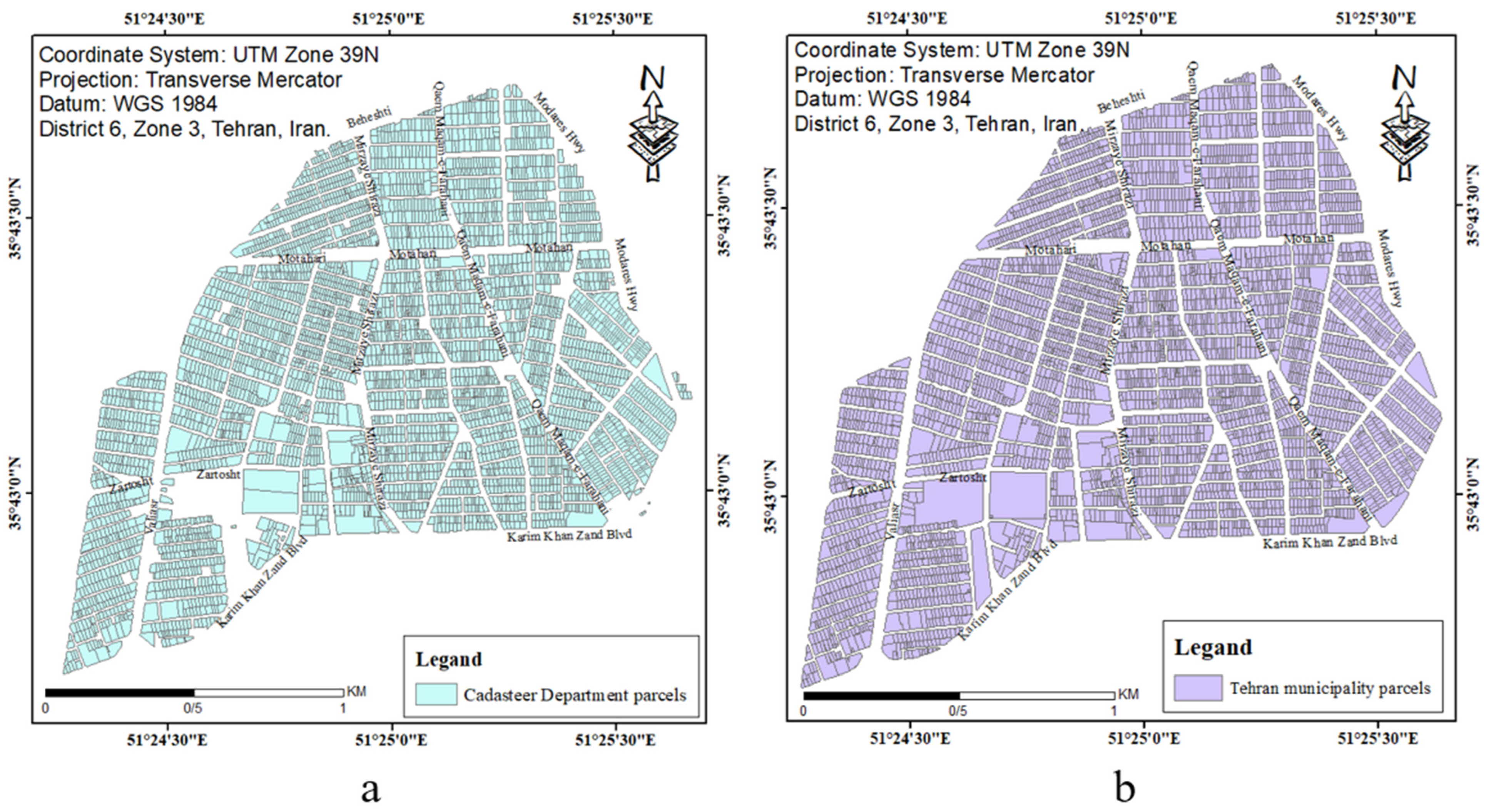
Figure 7 illustrates parcels in the Cadaster Department map and the Tehran Municipality map in the third zone of District Six after the preprocesses. The differences in the parcels and block numbers make it clear that some changes in the Cadaster Department map are essential for its enrichment.
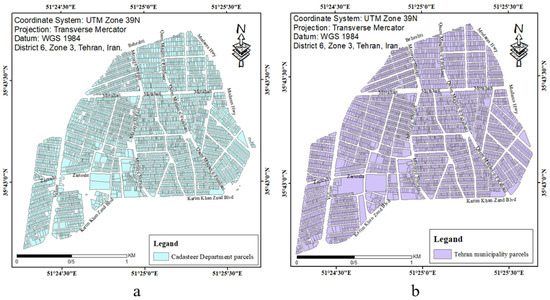
Figure 7.
Employed data after preprocesses. (a) The Cadaster Department map. (b) The Tehran Municipality map.
3.4. Matching
In order to evaluate the matching, test data had to be selected from all the different matching modes. Hence, after identifying the types of parcels in the first map based on the number of vertices, five percent of each type were considered as test data to validate the matching process. A total of 230 parcels were selected for the matching validation, which was about five percent of each state randomly considered in the study area. Figure 8 shows the selected parcels for the matching validation in the Cadaster Department (base) map.
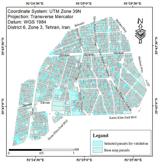
Figure 8.
The selected parcels for the matching validation.
After the matching process, the elements of the confusion matrix were calculated by test data, as shown in Table 5. According to the confusion matrix, the accuracy and F1-score of matching were equal to 0.952 and 0.975, which indicates that a high matching accuracy was achieved.

Table 5.
Matching validation.
In Table 5, confusion matrix elements have been defined as [41]:
- True Positives (TPs): correctly matched parcels;
- True Negatives (TNs): incorrectly matched parcels (the parcels were deleted in the second map while they were detected correctly by the algorithm);
- False Positives (FPs): incorrectly matched parcels;
- False Negatives (FNs): parcels that were not matched incorrectly (the parcels were not deleted in the second map but were not detected incorrectly by the algorithm).
3.5. Classification and Parcel Change Detection Modeling
Table 6 presents the parameters for tuning the models.

Table 6.
Tuning parameters.
The Cadaster Department map, which was used as the base map, has 4444 parcels, and the Tehran Municipality map, which was used as a more up-to-date and richer map, has 4468 parcels. In order to train and test the models, 25% of the data, which is equal to 1110 parcels of the Cadaster Department map, were divided into two categories of training and test data. A total of 70% of these data (777 parcels) were considered as training data and 30% (333 parcels) were considered as test data. After the matching, according to Table 1 and Figure 1 and Figure 3, some changes can be identified, including addition, deletion, integration (merging) and separation (splitting) of the parcels. For better training and testing of the models, parcels were selected from the integrated (merged), separated (split) and other parcels as training and test parcels. Table 7 shows the frequency of the different situations and the method used to select the training and test data.

Table 7.
Frequencies of different matching situations and the methods used to select the number of training and test parcels from the different situations.
The training and test data were spatially distributed in the study area shown in Figure 9.
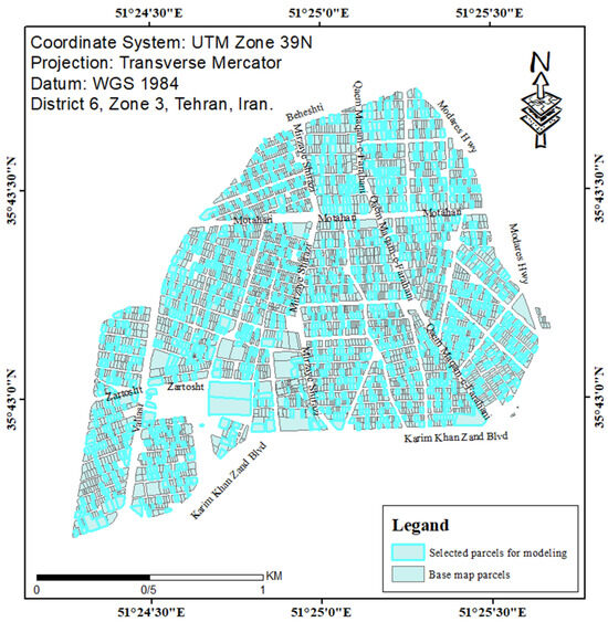
Figure 9.
The parcels selected as training and test data for modeling.
To evaluate the models, in each model, the test data and outputs were used to calculate the true positives, true negatives, false positives and false negatives. Finally, precision, recall, accuracy and F1-scores were calculated for each method. Table 8 shows the comparison of the models in terms of accuracy and F1-scores for the training and test data. In Table 8, SVM-GA and RF-GA are the models with feature selection, SVM-GA-GWO and RF-GA-GWO are the models with feature selection and grey wolf optimization, and SVM-GA-HHO and RF-GA-HHO are the models with feature selection and Harris hawks optimization.

Table 8.
Change detection modeling validation.
According to Table 8, the recalls of all the models are very high and close to one, which indicates the high ability of the models to identify the changes in the parcels of the Cadaster Department base map. The RF model has a higher accuracy and F1-score than the SVM model in both the GWO and HHO optimization modes, which indicates the greater ability of the RF model to detect changes and distinguish between changed parcels and unchanged ones compared to the SVM model. The SVM and RF models have the lowest accuracy among the models, which shows the effect of feature selection and hyperparameter optimization on improving accuracy of the models. Also, optimization by the Harris hawks optimization algorithm increased the F1-scores of the models compared to optimization by the grey wolf algorithm.
A list of features selected in each model is shown in Table 9. These features were selected by the feature selection algorithm (GA) in each model. The “N” indicates that the feature was not selected, and the “Y” indicates that the feature was selected in the desired model.

Table 9.
The parameters (features) selected in the models by feature selection.
According to Table 9, the features of the number of vertices (node count) of the parcels and the minimum extent Y of the parcels were selected in all the models, which indicates the importance of these features in detecting the changes in parcels with the research models. In addition, the features of centroid Y of the parcels, the polygon main angle of the parcels and MBB APodY1 were not selected in any of the models in the feature selection process, which indicates the lack of influence of these items in detecting changes in the parcels in the models. The selected features indicate the greater importance of geometric features compared to topologic and statistical features in detecting the parcel changes.
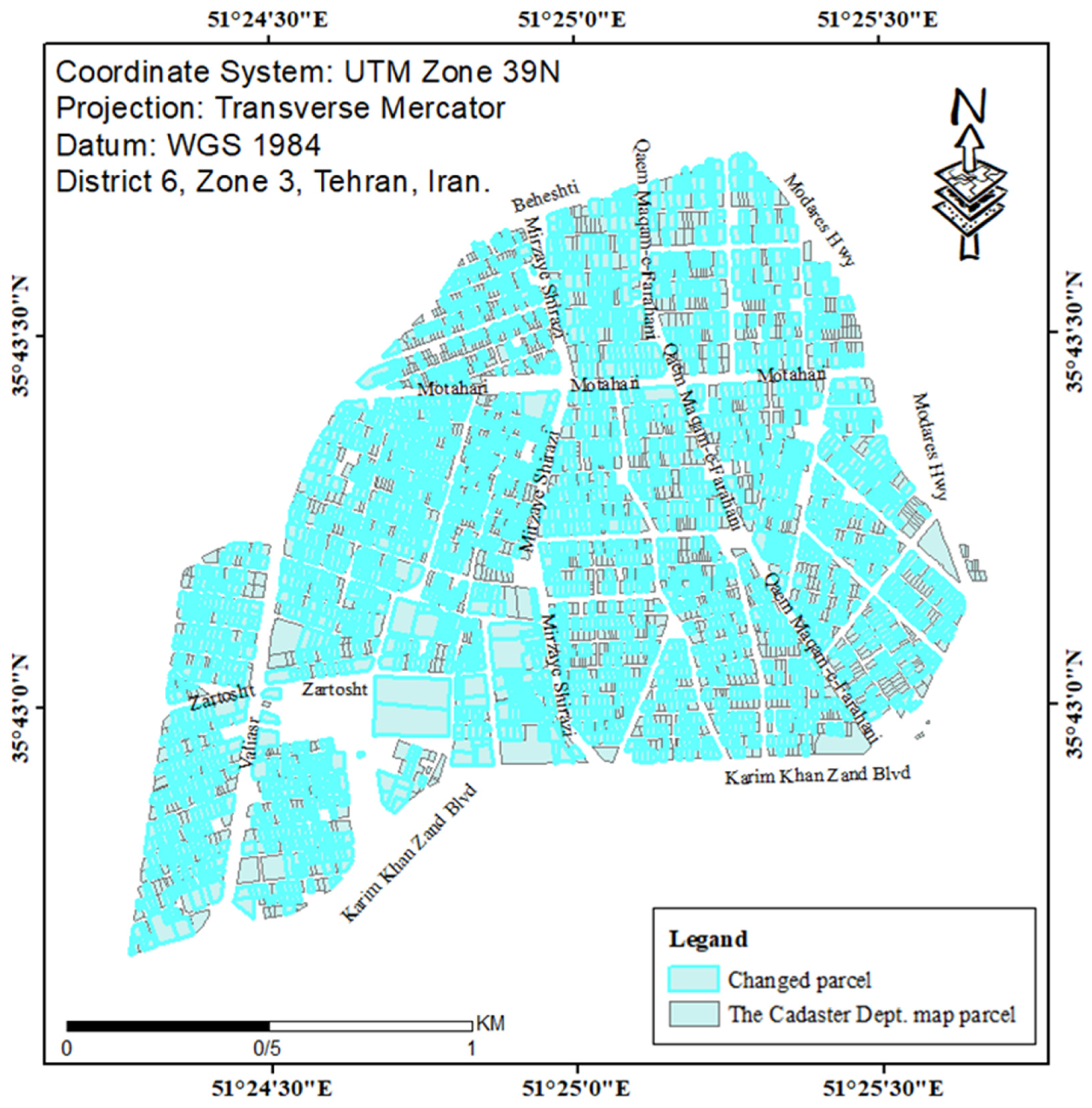
According to Table 8, the RF models with feature selection and GWO or HHO have better accuracy and F1-scores than the SVM ones. Based on the statistics of the confusion matrix in Table 8, the RF-GA-GWO model detected the changed parcels better than the RF-GA-HHO model. Hence, the RF-GA-GWO model was determined as the proposed model and implemented on the whole parcels of the base map. After training the model, other parcels that were not selected as training and test data were checked by the determined parameters and features, and the changes in the parcels were intelligently identified. Figure 10 illustrates the changed parcels detected by RF-GA-GWO. In this model, more than half of the parcels were detected as changed parcels, which indicates the existence of a number of changes in the base map and the need for its enrichment. The parcels detected via this method were used in the next section to enrich the base map.
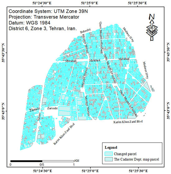
Figure 10.
The changed and detected parcels in the RF-GA-GWO model.
3.6. Base Map Enrichment
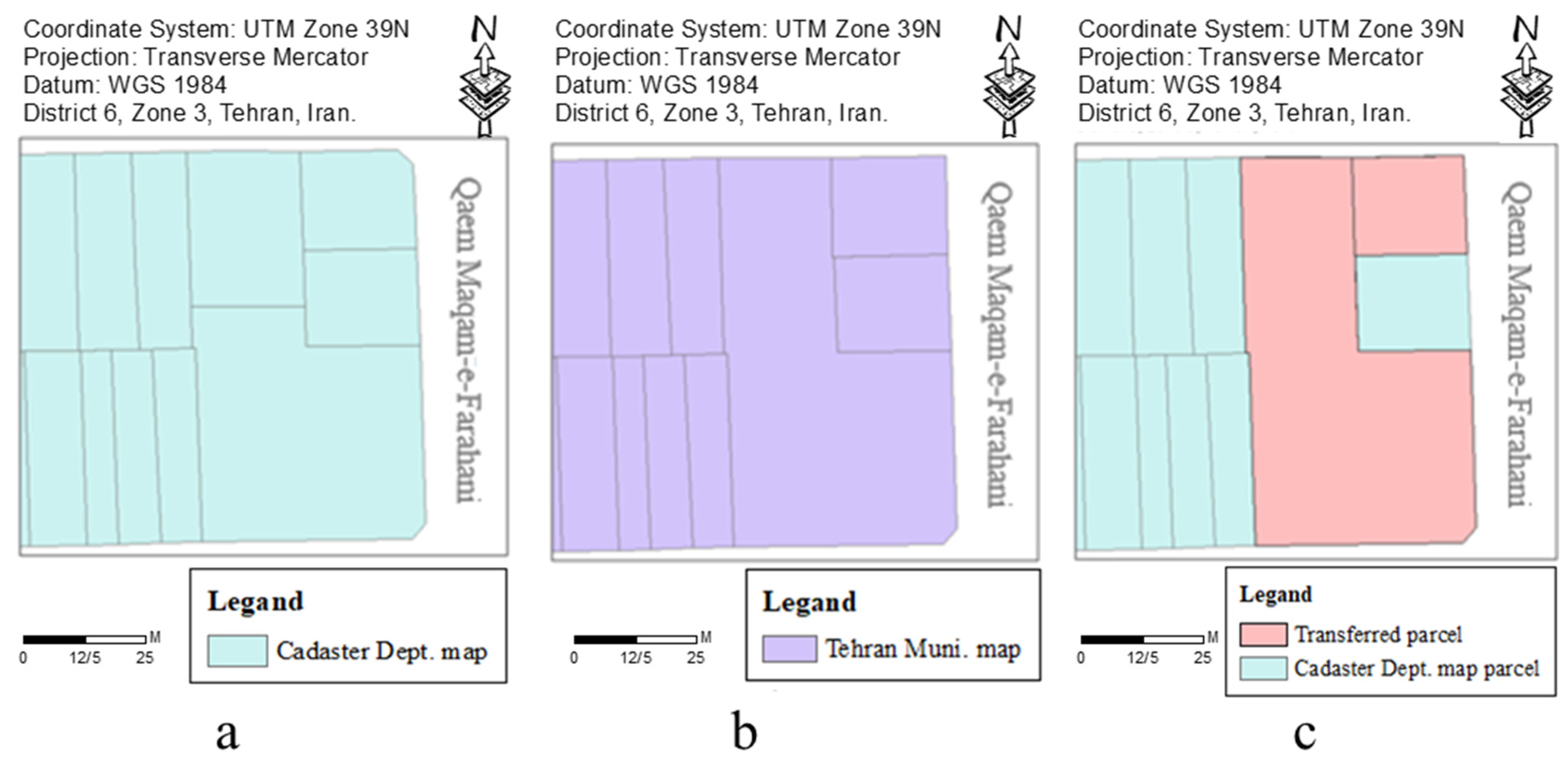
After the intelligent detection of the parcels in the Cadaster Deparment map that were changed according to the Tehran Municipality map and using data mining and machine learning methods, the enrichment of the base map was performed automatically. First, the detected changed parcels in the Cadaster Department map were removed. Then, by the neighbors of the parcels in the Tehran Municipality map and the transformation parameters, the corresponding parcels in the Tehran Municipality map were located in the Cadaster Department map. The transformation and placement of the parcels from the Tehran Municipality map to the Cadaster Department map were checked by the root mean square error (RMSE). After placing all the changed parcels, to evaluate the data enrichment, the topology of the parcels was checked. In cases of topologic errors, such as the overlaying of several parcels, the incorrectly located parcels were identified and corrected. Figure 11 presents an example of the identification of the changes in the Cadaster Department map and the location of the parcels from the Tehran Municipality map.
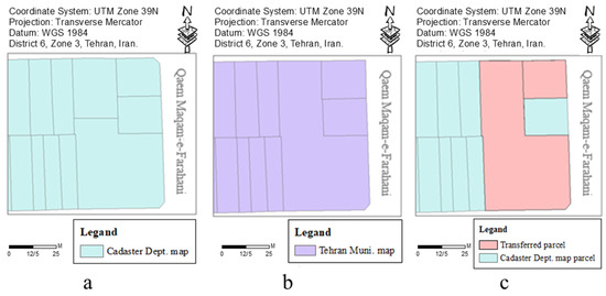
Figure 11.
The intelligent change detection and map enrichment in the base map. (a) The Cadaster Department map before enrichment. (b) The Tehran Municipality map. (c) The Cadaster Department map after the automatic enrichment.
According to Figure 11, in the displayed area, two changes were detected in the parcels of the Cadaster Department map. The detected changes included the merging of two parcels with each other and changes in the parcel geometry. The RMSEs of the merged parcels and the geometrically modified parcels were equal to 0.00051 and 0.000113 m, respectively.
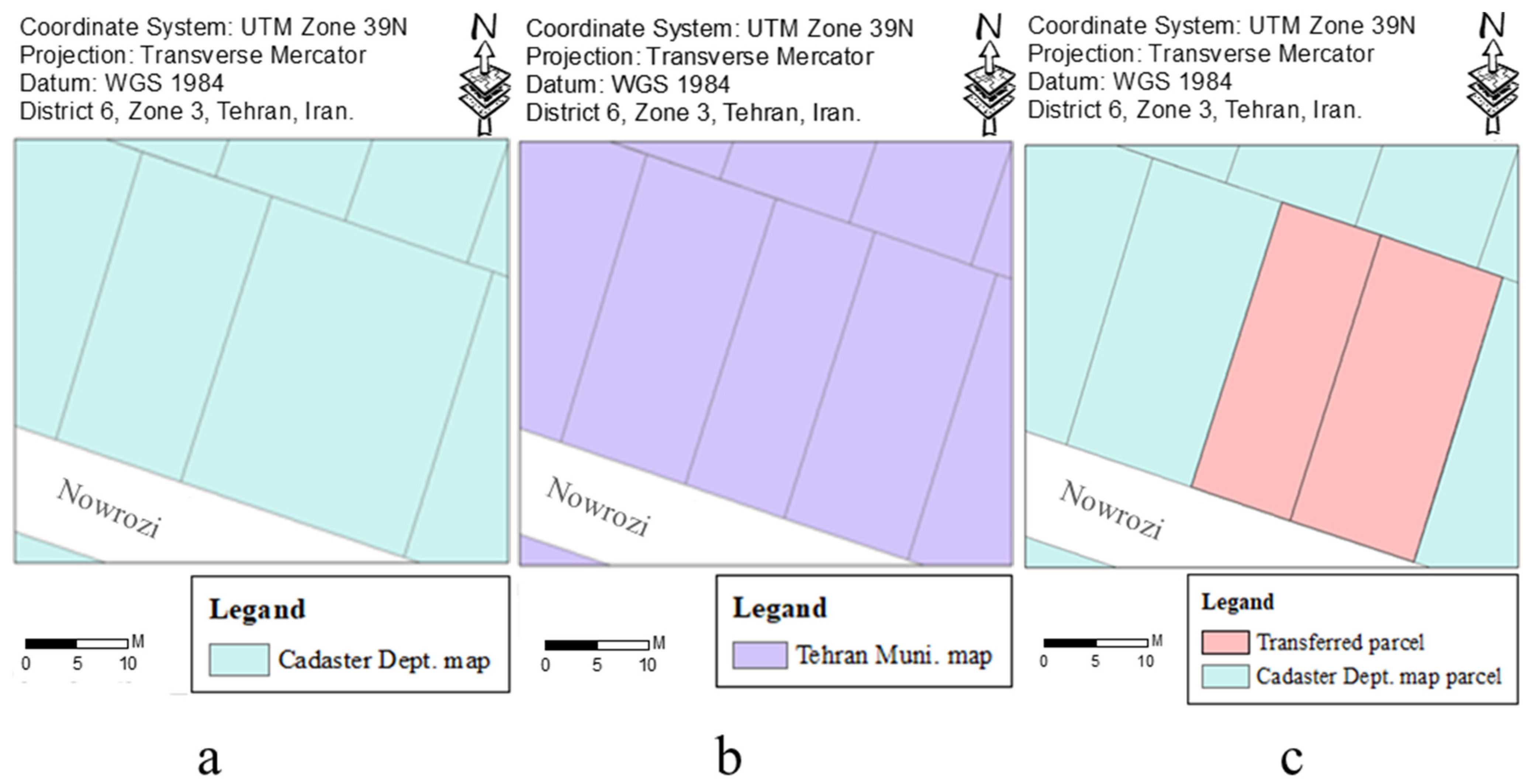
Figure 12 illustrates the intelligent detection of the separated parcels in the base map, as well as the automatic enrichment of the base map based on the transfer and placement of parcels from the Tehran Municipality map to the base map. The RMSE of the separated (split) parcel was equal to 0.000035 m.
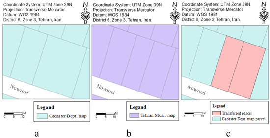
Figure 12.
The intelligent change detection and map enrichment in the base map. (a) The Cadaster Department map before enrichment. (b) The Tehran Municipality map. (c) The Cadaster Department map after the automatic enrichment.
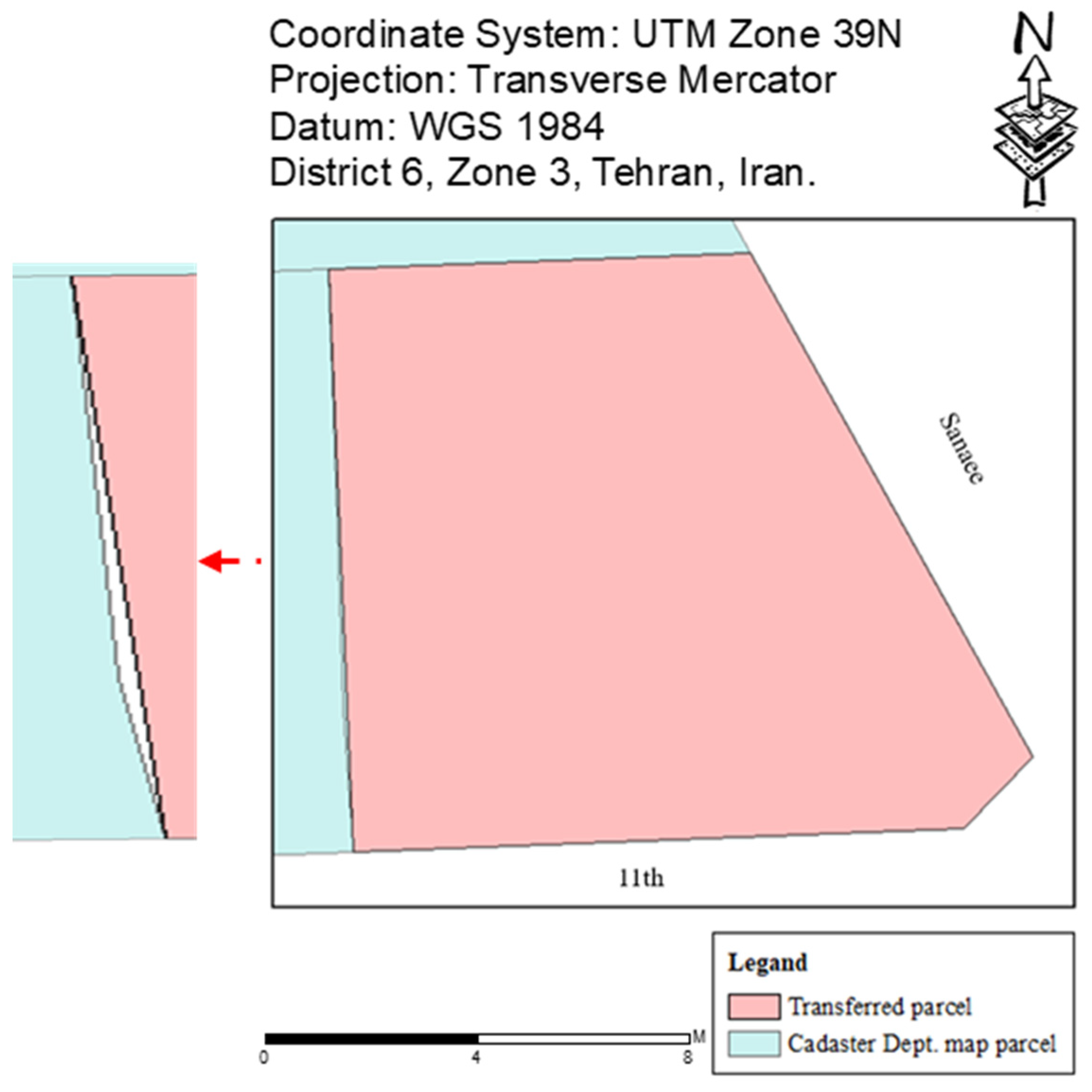
Figure 13 shows the topologic error (gap) caused by the removal of the changed parcel in the urban cadaster base map and its automatic enrichment. In these cases, the topologic error was resolved by correcting the parcel manually.
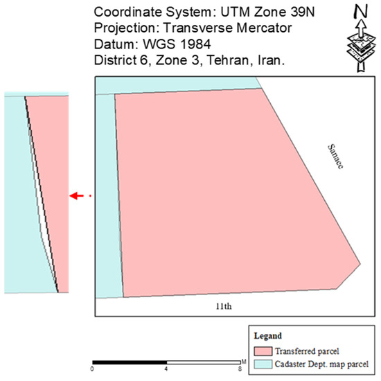
Figure 13.
The topologic error (gap) in the transformation and placement of the parcel from the Tehran Municipality map to the Cadaster Department map.
4. Discussion
The matching algorithm has an accuracy of 0.952 and an F1-score of 0.975. This method was able to identify the corresponding parcels with high accuracy. On the other hand, the use of the two-way matching caused more parcels to be correctly matched, and different states, including added and split parcels, were identified correctly and with high accuracy. Also, matching by the proposed method and identifying integrated (merged) and separated (split) parcels played an important role in training and validation in the modeling. Classifying the data by matching outputs caused a good selection for the training and test data, which had a suitable and random distribution among the different states of the parcels.
Using the feature selection and optimization of hyperparameters of the models improved the detection of changed parcels in the data and its accuracy. Feature selection led to selection of the best and most suitable features in each model. Based on the high and almost similar recalls of all the models, their ability to detect changes is very high. The RF models performed better than the SVM models due to the simultaneous and parallel implementation of several basic models with each other and finally using the majority vote to determine the result. The RF-GA-GWO and RF-GA-HHO models, with accuracies of 0.8541 and 0.8721, have the highest accuracies and ability to distinguish between changed and unchanged parcels. These models, with F1-scores equal to 0.9018 and 0.9109, have the highest F1-scores and ability to detect changes and the accuracy of detecting changes among the models employed in this research. The selected features in the models showed a greater influence of geometric features in detecting the changed parcels than topologic and statistical features. According to the confusion matrix in Table 4, feature selection and hyperparameter optimization effectively increased the rate of true predictions (true positives and true negatives) and also decreased false predictions (false negatives and false positives) in the proposed models. The RF-GA-GWO model had higher rates of true positives and false negatives, which increased the correct detection of the changed parcels. In contrast, the RF-GA-HHO model had higher rates of false positives and true negatives, which increased trust in the detected changed parcels. Hence, grey wolf optimization improved the ability of the RF algorithm to detect the changed parcels in the base map, while HHO improved the ability of the RF algorithm to detect the unchanged parcels in the base map. In general, in an area with a huge number of changed parcels, as in the base map compared to the more up-to-date map of the research study area, the RF-GA-GWO has a better performance than the RF-GA-HHO model in detecting these changes. Hence, the RF-GA-GWO model was selected as the proposed method in this research.
The automatic enrichment of the urban cadaster base map made it unnecessary to have experts check all the parcels and accelerated the enrichment of the maps. In addition, the parcels that were detected as false positives and considered as changed parcels by mistake were relocated by the proposed method. The strength of the models lay in detecting the changes in the parcels. In contrast, in detecting the unchanged parcels, they did not have the same performance as in detecting the changed parcels. Therefore, our proposed methodology more accurately covers false-positive cases in models and plays a significant role in the intelligent and automatic enrichment of maps. Automatic enrichment modified the shifting, rotation and scaling of the parcels in the Tehran Municipality map compared to those of the Cadaster Department map by affine transformation to replace the changed parcels in the base map. The existing topologic errors in the enrichment step were mostly due to the difference in the number of vertices (node counts) of the unchanged neighbors for each of the changed parcels in the two maps of Tehran Municipality and the Cadaster Department, which caused the overlapping of parcels or gaps between them. If the maps were correctly GIS readied and there were no extra vertices in the parcels, there would be fewer topologic errors in the automatic enrichment process.
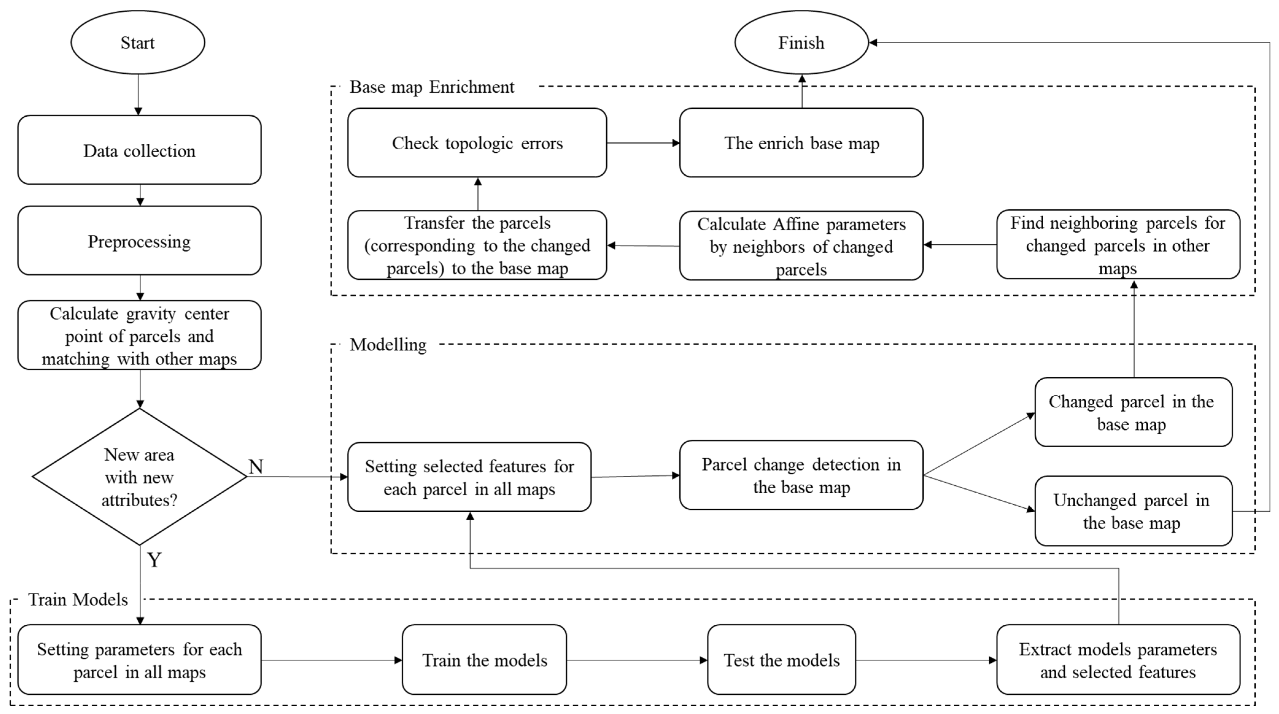
Figure 14 illustrates the intelligent and automatic framework developed in this research. First, available maps and data from different organizations are collected. Then, after preprocessing, the differences, inconsistencies and errors in the maps are resolved. By calculating the center of gravity of each parcel in the maps and transferring them to other maps, the corresponding parcels are identified in the other maps. If there are new information and features for the parcels, or if there is a specific geometric shape complexity for the parcels in the investigated area, the models are retrained by the training data. Finally, the selected features and modeling parameters are extracted for the other data. If the study area is similar to the previously studied area in which the model was trained, the selected parameters and features are used in the proposed model. After modeling all the parcels and detecting the changes in the whole area, the parcels from other maps that correspond to the changed parcels in the base map are placed in the base map by the affine transformation algorithm after calculating the affine parameters from unchanged neighbor parcels for each changed parcel, then the topologic errors are removed so that the base map is intelligently and automatically enriched.
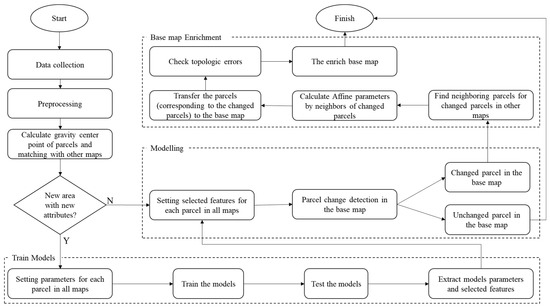
Figure 14.
The proposed framework for urban base map enrichment.
In this research, unlike previous studies [6,9,11], changes in a base map were identified by machine learning algorithms in an intelligent and automatic method, which increases the speed and accuracy of the urban map enrichment process. Moreover, relocating changed parcels automatically and updating them with the help of a more up-to-date map reduces human errors and the time required to enrich urban maps. In previous studies [6,9,11], enrichment has often been performed manually, visually and case by case, which is very time-consuming compared to the proposed model. The presented framework plays a very important role in reducing the cost and time spent by organizations in preparing urban maps or enriching urban cadastral maps by the quick and accurate use of available maps from other organizations. This framework solves some of the needs of organizations and lets them make more accurate and informed decisions.
Since the juridical map and registered parcels are fixed properties and obtained from the special administrative procedures, these parcels cannot be changed and replaced by other parcels without legal processing. In this research, the base map from the Cadaster Department was produced by the NCC and had no registered parcel. This base map is usually used beside another dataset for registered parcels to handle new requests for property registration. Hence, enriching this base map reduces the Cadastral Department process for registration. On the other hand, other organizations, such as utilities and infrastructure organizations, can effectively use the proposed framework to enrich their maps for better decision making and urban management.
5. Conclusions
The preparation of accurate cadastral maps in urban areas is a time-consuming and costly process for urban managent organizations. In addition, the enrichment and upgrading of maps by other organizations’ maps needs huge manpower, time and funding. Hence, intelligent and automatic enrichment of an existing map by the maps of other organizations and more up-to-date maps plays a vital role in informed urban management, enabling timely decisions with reduced costs. Since parcels are an important part of urban maps, an intelligent and automatic framework is essential to enrich two-dimensional maps of parcels in urban areas with urban maps of other organizations in the metropolises and cities of a country. This research focused on enrichment of the parcels in the Cadaster Department map from a geometric point of view and by the most up-to-date maps available in Tehran Municipality. After the data preprocessing, matching was performed by each parcel gravity center point and checking the position of the points in the other map. The matching process was implemented in both of the maps to find all types of matching and relations. To validate the process, five percent of the base map parcels were selected randomly based on the number of vertices of parcels. The accuracy and F1-scores were 0.952 and 0.975 for the matching algorithm. Based on different matching relations and different changes in the base map, 25 percent of the whole data (1110 parcels from 4444 parcels) were considered as training and test data. The training data included 70 percent of these data, and 30 percent of the data were considered as the test data. A total of 38 different geometric, topologic and statistical parameters were calculated for each parcel in both of the maps. After correlation matrix calculation, 19 parameters were selected for the modeling. Classification of the changed and unchanged parcels was implemented by SVM and RF algorithms. To improve the performance and accuracy of the models, feature selection by the GA and hyperparameter optimization by the GWO and HHO algorithms was performed in each model, which improved the accuracy of the models by about five percent and the F1-scores by about two percent. The proposed models were RF-GA-GWO and RF-GA-HHO. The RF-GA-GWO improved the model for detecting the changed parcels in the base map, and the RF-GA-HHO improved the model for detecting unchanged parcels in the base map. After training and validating the models, all data of the base map were classified into changed and unchanged parcels by the proposed models. The RF-GA-GWO model was selected for the base map enrichment phase, with more than 50 percent changed parcels in the modeling phase. In the base map enrichment step, the changed parcels were deleted from the base map and replaced with the corresponding parcels from the more up-to-date map automatically by neighbors of the changed parcels in both of the maps and affine transformation. Each parcel was evaluated by the RMSE of affine transformation and topology checking undertaken after the base map enrichment. Finally, an intelligent and automatic framework was proposed for map enrichment with a more up-to-date map by the machine learning algorithms.
Data access limitation was one of the main issues of this research. More information about parcels, such as owner’s names and land use. in each map may help to match the parcels better and cover other parts of map enrichment, such as semantics. Parcels with holes or parcels with their gravity centers located outside of their corresponding parcels in the other map may have caused errors in the matching process. There were none of these types of parcels in the study area; however, these parcels can be detected by point-in-polygon analysis, and the matching process can be corrected before the modeling. Since the accuracy and selected features in both of the models were close, the ensemble methods for integrating the models’ outputs were not very useful. Other models that cover other parts of feature space can be integrated with these models by ensemble algorithms, such as voting and stacking, to cover uncertainty [32].
In future research, we are going to consider other types of data in the maps to enrich the base map. In addition to the geometric point of view, other data like descriptive information can be considered. Another suggestion for future research is to use more complex transformations, such as projective transformation, to evaluate the accuracy of the enrichment phase. The outputs of the models can be integrated with each other by different algorithms, such as stacking and voting [32].
Author Contributions
Conceptualization, Alireza Hajiheidari, Mahmoud Reza Delavar and Abbas Rajabifard; methodology, Alireza Hajiheidari; software, Alireza Hajiheidari; validation, Alireza Hajiheidari; formal analysis, Alireza Hajiheidari; investigation, Alireza Hajiheidari; resources, Alireza Hajiheidari and Mahmoud Reza Delavar; data curation, Alireza Hajiheidari; writing—original draft preparation, Alireza Hajiheidari; writing—review and editing. Mahmoud Reza Delavar and Abbas Rajabifard; visualization, Alireza Hajiheidari; supervision, Mahmoud Reza Delavar and Abbas Rajabifard; project administration, Mahmoud Reza Delavar. All authors have read and agreed to the published version of the manuscript.
Funding
This research received no external funding.
Data Availability Statement
The datasets used and analyzed during the current study are available from the corresponding author on reasonable request.
Conflicts of Interest
The authors declare no conflict of interest.
References
- Molinero-Parejo, R.; Aguilera-Benavente, F.; Gómez-Delgado, M.; Shurupov, N. Combining a Land Parcel Cellular Automata (LP-CA) Model with Participatory Approaches in the Simulation of Disruptive Future Scenarios of Urban Land Use Change. Comput. Environ. Urban Syst. 2023, 99, 101895. [Google Scholar] [CrossRef]
- Hajji, R.; El Asri, H.; Ez-Zriouli, C. Upgrading to 3D Cadastre in Morocco: Lessons Learned from Benchmarking of International 3D Cadastral Systems. Land Use Policy 2023, 128, 106605. [Google Scholar] [CrossRef]
- Govedarica, M.; Radulović, A.; Sladić, D. Designing and Implementing a LADM-Based Cadastral Information System in Serbia, Montenegro and Republic of Srpska. Land Use Policy 2021, 109, 105732. [Google Scholar] [CrossRef]
- Tepe, E.; Safikhani, A. Spatio-Temporal Modeling of Parcel-Level Land-Use Changes Using Machine Learning Methods. Sustain. Cities Soc. 2023, 90, 104390. [Google Scholar] [CrossRef]
- Indrajit, A.; van Loenen, B.; Ploeger, H.; van Oosterom, P. Developing a Spatial Planning Information Package in ISO 19152 Land Administration Domain Model. Land Use Policy 2020, 98, 104111. [Google Scholar] [CrossRef]
- Bacior, S. Austrian Cadastre Still in Use—Example Proceedings to Determine the Legal Status of Land Property in Southern Poland. Land Use Policy 2023, 131, 106740. [Google Scholar] [CrossRef]
- Hajiheidari, A.R.; Delavar, M.R.; Rajabifard, A. Cadastral and urban maps enrichments using smart spatial data fusion. ISPRS Ann. Photogramm. Remote Sens. Spat. Inf. Sci. 2023, 10, 263–269. [Google Scholar] [CrossRef]
- Cienciała, A.; Sobolewska-Mikulska, K.; Sobura, S. Credibility of the Cadastral Data on Land Use and the Methodology for Their Verification and Update. Land Use Policy 2021, 102, 105204. [Google Scholar] [CrossRef]
- Ercan, O. Evolution of the Cadastre Renewal Understanding in Türkiye: A Fit-for-Purpose Renewal Model Proposal. Land Use Policy 2023, 131, 106755. [Google Scholar] [CrossRef]
- Negri, R.G.; Frery, A.C. A General and Extensible Framework for Assessing Change Detection Techniques. Comput. Geosci. 2023, 178, 105390. [Google Scholar] [CrossRef]
- Čeh, M.; Gielsdorf, F.; Trobec, B.; Krivic, M.; Lisec, A. Improving the Positional Accuracy of Traditional Cadastral Index Maps with Membrane Adjustment in Slovenia. ISPRS Int. J. Geo-Inf. 2019, 8, 338. [Google Scholar] [CrossRef]
- Safra, E.; Kanza, Y.; Sagiv, Y.; Doytsher, Y. Integrating Data from Maps on the World-Wide Web. In Proceedings of the International Symposium on Web and Wireless Geographical Information Systems, Hong Kong, China, 4–5 December 2006; Springer: Berlin/Heidelberg, Germany, 2006; pp. 180–191. [Google Scholar]
- Pullar, D.; Donaldson, S. Accuracy Issues for Spatial Update of Digital Cadastral Maps. ISPRS Int. J. Geo-Inf. 2022, 11, 221. [Google Scholar] [CrossRef]
- Song, A.-R.; Park, S.; Kim, Y.-I. Updating Cadastral Maps Using Deep Convolutional Networks and Hyperspectral Imaging; Daejeon Convention Center(DCC): Daejeon, Korea, 2019. [Google Scholar]
- Wierzbicki, D.; Matuk, O.; Bielecka, E. Polish Cadastre Modernization with Remotely Extracted Buildings from High-Resolution Aerial Orthoimagery and Airborne LiDAR. Remote Sens. 2021, 13, 611. [Google Scholar] [CrossRef]
- Ali, Z.; Tuladhar, A.; Zevenbergen, J. An Integrated Approach for Updating Cadastral Maps in Pakistan Using Satellite Remote Sensing Data. Int. J. Appl. Earth Obs. Geoinf. 2012, 18, 386–398. [Google Scholar] [CrossRef]
- Puniach, E.; Bieda, A.; Ćwiąkała, P.; Kwartnik-Pruc, A.; Parzych, P. Use of Unmanned Aerial Vehicles (UAVs) for Updating Farmland Cadastral Data in Areas Subject to Landslides. ISPRS Int. J. Geo-Inf. 2018, 7, 331. [Google Scholar] [CrossRef]
- Wang, S.; Li, W. GeoAI in Terrain Analysis: Enabling Multi-Source Deep Learning and Data Fusion for Natural Feature Detection. Comput. Environ. Urban Syst. 2021, 90, 101715. [Google Scholar] [CrossRef]
- Girard, N.; Charpiat, G.; Tarabalka, Y. Aligning and Updating Cadaster Maps with Aerial Images by Multi-Task, Multi-Resolution Deep Learning. In Proceedings of the 14th Asian Conference on Computer Vision, Perth, Australia, 2–6 December 2018; pp. 675–690, ISBN 978-3-030-20872-1. [Google Scholar]
- Fetai, B.; Grigillo, D.; Lisec, A. Revising Cadastral Data on Land Boundaries Using Deep Learning in Image-Based Mapping. ISPRS Int. J. Geo-Inf. 2022, 11, 298. [Google Scholar] [CrossRef]
- Nyandwi, E.; Koeva, M.; Kohli, D.; Bennett, R. Comparing Human Versus Machine-Driven Cadastral Boundary Feature Extraction. Remote Sens. 2019, 11, 1662. [Google Scholar] [CrossRef]
- Samal, A.; Seth, S.; Cueto, K. A Feature-Based Approach to Conflation of Geospatial Sources. Int. J. Geogr. Inf. Sci. 2004, 18, 459–489. [Google Scholar] [CrossRef]
- Kim, J.O.; Yu, K.; Heo, J.; Lee, W.H. A New Method for Matching Objects in Two Different Geospatial Datasets Based on the Geographic Context. Comput. Geosci. 2010, 36, 1115–1122. [Google Scholar] [CrossRef]
- Wang, Y.; Lv, H.; Chen, X.; Du, Q. A PSO-Neural Network-Based Feature Matching Approach in Data Integration. In Cartography-Maps Connecting the World; Springer: Berlin/Heidelberg, Germany, 2015; pp. 189–219. [Google Scholar] [CrossRef]
- Nürnberg, R. Calculating the Area and Centroid of a Polygon in 2d. 2013. Available online: http://wwwf.imperial.ac.uk/rn/centroid.pdf (accessed on 25 January 2024).
- Zhang, X.; Ai, T.; Stoter, J.; Zhao, X. Data Matching of Building Polygons at Multiple Map Scales Improved by Contextual Information and Relaxation. ISPRS J. Photogramm. Remote Sens. 2014, 92, 147–163. [Google Scholar] [CrossRef]
- Xavier, E.M.; Ariza-López, F.J.; Urena-Camara, M.A. A Survey of Measures and Methods for Matching Geospatial Vector Datasets. ACM Comput. Surv. 2016, 49, 1–34. [Google Scholar] [CrossRef]
- Awad, M.; Khanna, R. Support Vector Regression. In Efficient Learning Machines; Springer: Berlin/Heidelberg, Germany, 2015; pp. 67–80. [Google Scholar]
- Wu, X.; Kumar, V.; Ross Quinlan, J.; Ghosh, J.; Yang, Q.; Motoda, H.; McLachlan, G.J.; Ng, A.; Liu, B.; Yu, P.S. Top 10 Algorithms in Data Mining. Knowl. Inf. Syst. 2008, 14, 1–37. [Google Scholar] [CrossRef]
- Smola, A.J.; Schölkopf, B. A Tutorial on Support Vector Regression. Stat. Comput. 2004, 14, 199–222. [Google Scholar] [CrossRef]
- Han, J.; Kamber, M.; Pei, J. Data Mining: Concepts and Techniques, 3rd ed.; Morgan Kaufmann: Burlington, MA, USA, 2012. [Google Scholar]
- Zhang, C.; Ma, Y. Ensemble Machine Learning: Methods and Applications; Springer: Berlin/Heidelberg, Germany, 2012; ISBN 1-4419-9325-8. [Google Scholar]
- Kuncheva, L.I. Combining Pattern Classifiers: Methods and Algorithms; John Wiley & Sons: Hoboken, NJ, USA, 2014; ISBN 1-118-31523-5. [Google Scholar]
- Liaw, A.; Wiener, M. Classification and Regression by randomForest. R News 2002, 2, 18–22. [Google Scholar]
- Mirjalili, S.; Dong, J.S.; Lewis, A. Nature-Inspired Optimizers; Springer: Cham, Switzerland, 2020; pp. 69–85. [Google Scholar]
- Haupt, R.L.; Haupt, S.E. Practical Genetic Algorithms; John Wiley & Sons: Hoboken, NJ, USA, 2004; ISBN 0-471-67175-4. [Google Scholar]
- Srinivas, M.; Patnaik, L.M. Genetic Algorithms: A Survey. Computer 1994, 27, 17–26. [Google Scholar] [CrossRef]
- Mirjalili, S.; Mirjalili, S.M.; Lewis, A. Grey Wolf Optimizer. Adv. Eng. Softw. 2014, 69, 46–61. [Google Scholar] [CrossRef]
- Heidari, A.A.; Mirjalili, S.; Faris, H.; Aljarah, I.; Mafarja, M.; Chen, H. Harris Hawks Optimization: Algorithm and Applications. Future Gener. Comput. Syst. 2019, 97, 849–872. [Google Scholar] [CrossRef]
- Chai, T.; Draxler, R.R. Root Mean Square Error (RMSE) or Mean Absolute Error (MAE)?—Arguments against Avoiding RMSE in the Literature. Geosci. Model Dev. 2014, 7, 1247–1250. [Google Scholar] [CrossRef]
- Chicco, D.; Jurman, G. The Advantages of the Matthews Correlation Coefficient (MCC) over F1 Score and Accuracy in Binary Classification Evaluation. BMC Genom. 2020, 21, 6. [Google Scholar] [CrossRef]
- Powers, D.M. Evaluation: From Precision, Recall and F-Measure to ROC, Informedness, Markedness and Correlation. arXiv 2020, arXiv:2010.1606. [Google Scholar]
- Gray, A.; Abbena, E.; Salamon, S. Modern Differential Geometry of Curves and Surfaces with Mathematica. 2006. Available online: https://hdl.handle.net/2318/104908 (accessed on 25 January 2024).
- Tehran Municipality. Tehran Statistical Yearbook 2021–2022; Information and Communication Technology Organization of Tehran Municipality: Theran, Iran, 2022. [Google Scholar]
- Hajiheidari, A.; Delavar, M.R.; Rajabifard, A. Challenges of Integrating Cadastral Map and Urban Data Infrastructure in Iran, 4th ed.; International Geoinformation Days (IGD): Tabriz, Iran, 2022; pp. 155–158. [Google Scholar]
- Mohammadi, H. The Integration of Multi-Source Spatial Datasets in the Context of SDI Initiatives; University of Melbourne: Melbourne, Australia; Centre for Spatial Data Infrastructures and Land Administration: Carlton, Australia, 2008. [Google Scholar]
- Song, X.; Cheng, C.; Zhou, C.; Zhu, D. Gestalt-Based Douglas-Peucker Algorithm to Keep Shape Similarity and Area Consistency of Polygons. Sens. Lett. 2013, 11, 1015–1021. [Google Scholar] [CrossRef]
- National Cartographic Center of Iran. Standards and Instructions for Public Display and Cartography; National Cartographic Center of Iran: Tehran, Iran, 2012. [Google Scholar]
- National Cartographic Center of Iran. Multi-Scale Spatial Data Model; National Cartographic Center of Iran: Tehran, Iran, 2021. [Google Scholar]
Disclaimer/Publisher’s Note: The statements, opinions and data contained in all publications are solely those of the individual author(s) and contributor(s) and not of MDPI and/or the editor(s). MDPI and/or the editor(s) disclaim responsibility for any injury to people or property resulting from any ideas, methods, instructions or products referred to in the content. |
© 2024 by the authors. Licensee MDPI, Basel, Switzerland. This article is an open access article distributed under the terms and conditions of the Creative Commons Attribution (CC BY) license (https://creativecommons.org/licenses/by/4.0/).


