Article

Hourly PM2.5 Concentration Prediction Based on Empirical Mode Decomposition and Geographically Weighted Neural Network

School of Geodesy and Geomatics, Wuhan University, Wuhan 430079, China
*
Author to whom correspondence should be addressed.
ISPRS Int. J. Geo-Inf. 2024, 13(3), 79; https://doi.org/10.3390/ijgi13030079
Submission received: 3 January 2024 / Revised: 15 February 2024 / Accepted: 26 February 2024 / Published: 2 March 2024
(This article belongs to the Special Issue HealthScape: Intersections of Health, Environment, and GIS&T)

Abstract

:
Accurate prediction of fine particulate matter (PM2.5) concentration is crucial for improving environmental conditions and effectively controlling air pollution. However, some existing studies could ignore the nonlinearity and spatial correlation of time series data observed from stations, and it is difficult to avoid the redundancy between features during feature selection. To further improve the accuracy, this study proposes a hybrid model based on empirical mode decomposition (EMD), minimal-redundancy-maximal-relevance (mRMR), and geographically weighted neural network (GWNN) for hourly PM2.5 concentration prediction, named EMD-mRMR-GWNN. Firstly, the original PM2.5 concentration sequence with distinct nonlinearity and non-stationarity is decomposed into multiple intrinsic mode functions (IMFs) and a residual component using EMD. IMFs are further classified and reconstructed into high-frequency and low-frequency components using the one-sample t-test. Secondly, the optimal feature subset is selected from high-frequency and low-frequency components with mRMR for the prediction model, thus holding the correlation between features and the target variable and reducing the redundancy among features. Thirdly, the residual component is predicted with the simple moving average (SMA) due to its strong trend and autocorrelation, and GWNN is used to predict the high-frequency and low-frequency components. The final prediction of the PM2.5 concentration value is calculated by an artificial neural network (ANN) composed of the predictive values of each component. PM2.5 concentration prediction experiments in three representational cities, such as Beijing, Wuhan, and Kunming were carried out. The proposed model achieved high accuracy with a coefficient of determination greater than 0.92 in forecasting PM2.5 concentration for the next 1 h. We compared this model with four baseline models in forecasting PM2.5 concentration for the next few hours and found it performed the best in PM2.5 concentration prediction. The experimental results indicated the proposed model can improve prediction accuracy.

1. Introduction

The United Nations Sustainable Development Goals (SDGs) are a set of 17 social, economic and environmental goals set by the United Nations in 2015 to address global challenges and achieve sustainable development [1]. One of them is to build inclusive, safe, resilient, and sustainable cities and human settlements. However, amid the expeditious economic and societal advancement, the worldwide ecological milieu has suffered tremendous harm, precipitating a notable catalyst in compromising human well-being—air quality degradation [2,3]. The deleterious impacts of air pollution on human health are unequivocal [4]. The main culprit is fine particulate matter (PM2.5) [5], with ramifications extending beyond its adverse effects on air quality and visibility. PM2.5 harbors toxic and detrimental substances that permeate deep within the lungs, heart, and bloodstream, exerting a pernicious influence on vital organs such as the heart and brain, which poses a grave menace to human health [5,6,7]. The precise forecasting of PM2.5 concentration is crucial to ameliorating environmental conditions, effectively managing air pollution, and proactively averting the myriad health afflictions triggered by atmospheric contamination [8,9,10].
Recent research methodologies employed for PM2.5 concentration prediction can be broadly classified into three main categories: mechanistic, statistical, and artificial intelligence models [11,12]. Mechanistic models leverage meteorological principles and mathematical techniques to simulate air quality at specific scales [9,12]. Typical mechanistic models include the Community Multiscale Air Quality (CMAQ) model [13,14] and the Weather Research and Forecasting (WRF) model [15,16]. High computational requirements and complex modeling processes are among the factors that impede the broader utilization of mechanistic models [12,13,14,15,16,17]. Statistical models explore the dynamics of PM2.5 using statistical analysis techniques, which are devoid of modeling intricacies, yet display superior performances [18,19]. Statistical models primarily include the autoregressive moving average model (ARMA) [20,21] and the autoregressive integrated moving average model (ARIMA) [22]. The reliance of statistical models on historical PM2.5 concentration data poses a challenge when incorporating external factors into the analysis [23]. Additionally, statistical models struggle to capture the nonlinear characteristics present in PM2.5 concentration effectively [12]. Artificial intelligence models mainly include machine learning and deep learning [23]. For instance, He et al. [24] employed an artificial neural network (ANN) to forecast PM2.5 concentration. Experiments indicated that the ANN successfully captured the nonlinear relationship between PM2.5 and the input variables.
The rapid advancement of deep learning technology has garnered significant scholarly acclaim while simultaneously being used for air quality forecasting [12]. Long short-term memory neural networks (LSTMs) [25,26] and convolutional neural networks (CNNs) [27] represent two extensively utilized deep learning architectures within the domain of air quality prediction. Li et al. [8] introduced a hybrid model that combined CNN and LSTM to predict the 24-h PM2.5 concentration in Beijing. Previous research [25,26,27] has demonstrated the commendable predictive capabilities of deep learning in discerning PM2.5 concentration with the utmost precision. Nonetheless, most existing deep learning models have struggled to advance beyond their current performance, primarily due to their inadvertent disregard for the non-stationarity inherent in time series [28]. Considering the detailed nature of PM2.5 sequences, delving into data preprocessing techniques for PM2.5 prediction has become imperative. These approaches have exhibited promising achievements, contributing to a discernible enhancement in prediction accuracy [29]. The adoption of data decomposition techniques is effective for preprocessing PM2.5 time series data, with the potential to advance the accuracy of PM2.5 concentration prediction significantly [30]. Most data decomposition techniques are based on empirical mode decomposition (EMD) [28,31]. For instance, Huang et al. [28] demonstrated the efficacy of employing EMD to decompose the initial PM2.5 sequence into multiple subsequences. Subsequently, they applied a well-constructed gated recurrent unit (GRU) to forecast each subsequence. The predicted value of each subsequence was aggregated to yield the final predicted value of PM2.5 concentration. Numerous previous studies [28,29,30,31] have confirmed the efficacy of data decomposition techniques in enhancing the accuracy of air quality predictions. Hence, the model proposed in this study employs EMD to preprocess the original PM2.5 sequence into multiple intrinsic mode functions (IMFs). Subsequently, the IMFs are reconstructed based on the one-sample t-test. This approach reduces the model’s complexity and runtime while maintaining prediction accuracy.
Feature selection contributes to improved model performance and reduced model complexity [32]. For PM2.5 concentration prediction, several common feature selection criteria were utilized, including the Pearson correlation coefficient [33], Kendall’s tau coefficient [34], causality [32], and mutual information [35]. While these feature selection methods perform well in selecting features that are highly relevant to the target variable, they may still face challenges in avoiding redundancy between the selected features. The minimal-redundancy-maximal-relevance (mRMR) algorithm considers both the redundancy between features and their relevance to the target variable [36]. Consequently, the model proposed in this study utilizes the mRMR algorithm for feature selection.
Considering the data from neighboring stations surrounding the target station can further improve the prediction accuracy [18]. Geographically weighted regression (GWR) is a spatial statistical analysis method for exploring spatial non-stationarity and spatial relationships in geographic data [37]. Combining the idea of GWR and ANN, this study proposes the novel geographically weighted neural network (GWNN) model for predicting PM2.5 concentration. GWNN model leverages the capabilities of ANN to determine the coefficients of GWR, thereby eliminating the issue of traditional methods for tedious kernel function and bandwidth selection.
Combining data decomposition, data reconstruction, feature selection, and considering the spatial relationship of PM2.5 monitoring stations, this study proposes a hybrid model called EMD-mRMR-GWNN for PM2.5 concentration prediction. The main contributions of this study are as follows:
  • The analysis of PM2.5 concentration in three representative cities, such as Beijing, Wuhan, and Kunming, reveals that the PM2.5 concentration has distinct nonlinearity as well as the diversity of seasonal patterns.
  • The EMD-mRMR-GWNN model was developed for PM2.5 concentration prediction. This model effectively integrates the advantages of data decomposition, data reconstruction, and feature selection techniques while considering the spatial relationship of PM2.5 monitoring stations. Experimental results on datasets from three cities in China (Beijing, Wuhan, and Kunming) indicate that the proposed hybrid model performed well.
  • The original PM2.5 sequence is adaptively decomposed into multiple IMFs and a residual component using EMD and classified into high-frequency and low-frequency components by the one-sample t-test, significantly reducing the prediction difficulty and model complexity.
  • For prediction accuracy, considering the correlation between features and the target variable, as well as the redundancy among features, we utilize the mRMR to select the optimal feature subset. By leveraging the nonlinear modeling capability of ANN and the spatial correlation capturing ability of GWR, we build a GWNN model to predict the high-frequency and low-frequency components, which significantly improves the accuracy of PM2.5 prediction.
This study is structured as follows: Section 2 introduces the material of this study and presents the modeling framework. Section 3 analyzes the performance of the EMD-mRMR-GWNN model and compares it with LSTM, GRU, GWNN, and mRMR-GWNN models. Finally, a conclusion is provided in Section 4.

2. Materials and Methods

2.1. Data Description

Three Chinese cities were selected as the study areas: Beijing, Wuhan, and Kunming. Beijing has 12 air quality monitoring stations (1001A–1012A), Wuhan has 9 (1325A–1334A, of which 1332A was excluded due to too many missing values), and Kunming has 6 (1450A–1455A). These cities were chosen to represent different geographical regions and varying levels of air pollution. Thus, the study provided a more comprehensive understanding of PM2.5 concentration prediction in diverse urban environments. The distribution of air quality monitoring stations in these three cities is shown in Figure 1.
The air quality data were obtained from the China National Environmental Monitoring Centre (CNEMC). Hourly pollutant concentration data, including PM2.5, PM10, SO2, NO2, O3, and CO, were collected from air quality monitoring stations in Beijing, Wuhan, and Kunming. The data collection period spanned from 1 January 2016, to 31 December 2020.
Figure S1 shows the PM2.5 concentration sequences of Beijing, Wuhan, and Kunming (one station is shown per city). Table S1 shows the statistical data of PM2.5 concentrations. The PM2.5 concentrations in all three cities exhibited volatility and had significantly different characteristics. The average PM2.5 concentration in Beijing was high and very volatile. In contrast, Kunming maintained a low average PM2.5 concentration with little volatility, resulting in stable air quality. Wuhan’s air quality was intermediate between the first two cities, with moderate PM2.5 concentration and volatility. Overall, these three cities displayed a declining trend in PM2.5 concentration, indicating an improvement in air quality. One possible reason was that the Chinese government has made significant efforts to adjust the energy structure, industrial structure, and transportation structure. In recent years, the Chinese Government has taken positive action on many fronts to achieve the goal of sustainable development. First, it has promoted energy transformation, limiting the use of highly polluting coal energy and encouraging clean energy alternatives [38]. Second, the Chinese government has actively promoted industrial upgrading and transformation to reduce dependence on resource-intensive and highly polluting industries. Finally, the Chinese government focuses on public transport in urban planning, building convenient public transport systems such as subways and light railways, and supporting the development of new energy vehicles through policies such as subsidies for car purchases [39]. Figure S2 shows the PM2.5 concentration for each season from December 2019 to November 2020 at the three stations. For Beijing and Wuhan, the highest PM2.5 concentrations were in winter, and the lowest were in summer. Heating is one of the major reasons for the high PM2.5 concentration during winter in Beijing. Wuhan has predominantly northerly winds in winter, thus the transmission of pollutants from centralized heating in the north may contribute to air pollution in Wuhan. The seasonal characteristics of PM2.5 in Kunming were different from those in Wuhan and Beijing. The PM2.5 concentration in Kunming was greatest during spring. Possible causes were spring drought, large temperature differences between day and night, scarce rainfall, and being prone to inversions and fog, which affected the dispersion of PM2.5. In this study, the three cities were considered representative as they corresponded to regions with high, moderate, and low PM2.5 concentrations, respectively. The proposed model’s stability was verified using different PM2.5 concentration datasets.

2.2. Empirical Mode Decomposition

EMD is a data analysis method used to decompose a nonstationary signal into a set of IMFs and a residual component. Each IMF has a specific frequency range. EMD is an adaptive data decomposition method that does not require predefined basis functions or filters [40]. The EMD implementation process is as follows:
  • Detect and extract the local maximum and local minimum in the signal x(t) and set the initial index i = 1 .
  • The upper envelope u(t) and lower envelope l(t) of the signal are obtained by cubic spline interpolation of the envelope between the extreme points.
  • Calculate the mean value m(t) of the upper and lower envelope.
    m t = u t + l t 2
  • The mean value m(t) of the upper and lower envelope is removed from the original signal x(t) to obtain a new sequence h(t).
    h t = x t m t
  • A judgment is made on the new sequence h(t). If h(t) satisfies the following two conditions: the number of extreme points and the number of points crossing the zero point are equal or differ by no more than one, and the average value of the upper envelope formed by the local extreme points and the lower envelope formed by the local extreme points is zero, then h(t) is considered to be an IMF, I M F i t = h ( t ) . If h(t) does not satisfy the above conditions, h(t) is considered the original signal for the next round of iterations until the conditions are satisfied.
  • The above steps are repeated until no more new IMFs can be decomposed, and the remaining signal is regarded as the residual component Res(t).
  • Finally, the original signal is decomposed into multiple IMFs and a residual component.
    x t = n = 1 i I M F i t + R e s t

2.3. Minimal-Redundancy-Maximal-Relevance

The mRMR (minimal-redundancy-maximal-relevance) is a feature selection method used to select the most representative subset of features from a given feature set that is highly correlated with the target variable and has less redundancy [36]. The mRMR algorithm evaluated the importance of each feature by measuring its relevance and redundancy. The goal of the mRMR algorithm was to reduce redundancy in the subset of features while maintaining high correlation.

2.3.1. Maximal Relevance

According to mRMR, maximal relevance is achieved by finding a subset of features that satisfies Equation (4), maximizing the average of the mutual information between the features in the subset of features and the target variable.
max D = 1 K x i K I x i ; y
where K is the subset of features, x i is the feature, and y is the target variable. I is the mutual information between the feature x i and the target variable y, and D is the average of the mutual information between the features and the target variable in the subset of features.
Mutual information is a concept used to measure the correlation between two random variables [36] to capture and assess the interdependence between these variables by evaluating the amount of information one variable provides about another variable [41]. Specifically, for two discrete random variables x and y, their mutual information is defined as:
I x ; y = p x , y l o g p x , y p x p y d x d y
where p x , y denotes the joint probability distribution of x and y, and p(x) and p(y) denote the marginal probability distribution of x and y, respectively. A larger value of mutual information indicates a stronger correlation between the two variables. A value of 0 indicates that the two variables are independent.

2.3.2. Minimal Redundancy

When selecting a subset of features based on the maximal relevance criterion, a significant amount of redundant information may be generated within the chosen features. This redundancy can adversely affect the computational effort required by the model and potentially decrease the prediction accuracy [36]. Consequently, eliminating the redundant information to optimize the selected subset of features becomes necessary. According to the mRMR, minimal redundancy is achieved by minimizing the mutual information between features in the subset as follows:
min R = 1 K 2 x i , x j K I x i ; x j
where K is the subset of features, x i and x j are the features in the subset, and I is the mutual information between the features. Redundant information is removed by minimizing mutual information between features.
Ultimately, considering both the relevance between the features and the target variable, and the redundancy between the features, the goal of the mRMR is to satisfy Equation (7).
max Φ = D R
Φ denotes the difference between the relevance and the redundancy. By maximizing the difference between relevance and redundancy, the mRMR can reduce redundancy in the subset of features while maintaining high relevance. The mRMR finds a subset of features through an incremental search. Suppose that the n − 1 features were selected from the original feature set X, constituting the subset of features K n 1 , then the selection of the nth feature x n needs to satisfy Equation (8).
m a x x n X K n 1 I x n ; y 1 n 1 x i K n 1 I x n ; x i
According to Equation (8), the mRMR successively selects features from the remaining set of features XK and adds them to the subset of features K. Finally, the subset of features with the largest mRMR value is selected as the model input.

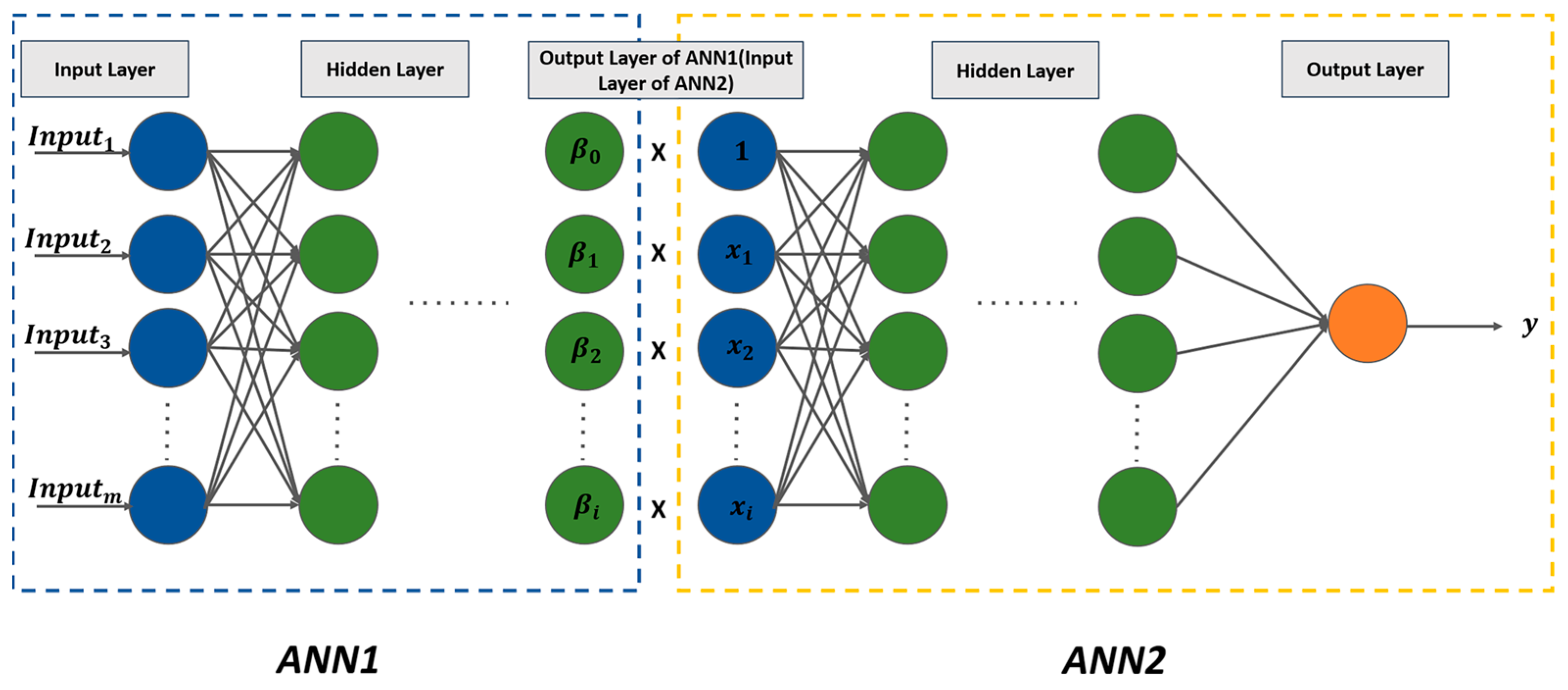
2.4. Geographically Weighted Neural Network

The PM2.5 concentration sequence is nonstationary and a nonlinear relationship exists between PM2.5 and the dependent variables. However, the GWR model is a linear model that does not address the nonlinear relationship inherent in the data. Furthermore, the GWR model relies solely on the spatial distance and the spatial weight matrix generated by the kernel function to calculate the model, which is insufficient for capturing and explaining the intricate relationship between the dependent variable and the independent variables [37]. In addition, the selection of an appropriate kernel function posed a challenge. Therefore, when it comes to predicting PM2.5 concentration, relying solely on the GWR model was unreliable. ANN possessed a more robust capability for nonlinear modeling compared to traditional linear models. By incorporating a hierarchical structure and activation functions, ANN effectively captured and represented intricate nonlinear relationships among input features [42]. Furthermore, ANN learned from extensive amounts of data and dynamically adjusted model parameters to suit various problems. To exploit the benefits of both ANN and GWR, we proposed the GWNN model for predicting PM2.5 concentration. The GWNN model integrated the geographically weighted conception into ANN to enhance the accuracy of PM2.5 concentration prediction. By combining the robust nonlinear modeling capabilities of ANN with the spatial correlation capturing abilities of GWR, GWNN aimed to improve the accuracy and reliability of PM2.5 concentration prediction. The structure of GWNN is shown in Figure 2.
GWNN consisted of two ANNs with different roles. The ANN1 is a coefficient estimation neural network used to learn the coefficients β in GWR. Any reasonably defined distance metric can be used for GWR model solving [43]. Simple spatial distances could not express the complex spatial relationships between stations. Consequently, we designated the PM2.5 concentration data from neighboring stations surrounding the target station within the previous 24 h of the prediction time as the ANN1 input. This was used to capture the spatial relationship of PM2.5 concentration among different stations. The ANN1 output was the regression coefficient β. The product of the regression coefficient β (learned by ANN1) and the dependent variable x was employed as input to the second neural network, ANN2. The independent variable x contained the constant 1 and the features selected by the mRMR. Through the nonlinear transformation, ANN2 provided the predicted output value, y. Both ANN1 and ANN2 consisted of an input layer, multiple hidden layers, and an output layer.

2.5. Proposed Model

Based on data decomposition, mRMR, and GWNN, this study proposed a hybrid model EMD-mRMR-GWNN for PM2.5 concentration prediction, as shown in Figure 3. The EMD reduced the non-stationarity of the original PM2.5 sequence by decomposing it into a set of subsequences. Additionally, the one-sample t-test was introduced to classify and reconstruct the subsequences into high-frequency component and low-frequency components. The mRMR was used to select features that were highly correlated with the target variable and had less redundancy. This approach aimed to reduce model complexity while improving prediction accuracy. GWNN was used for predicting high-frequency and low-frequency components. GWNN integrated the geographically weighted idea into ANN, leveraging the nonlinear modeling capabilities of ANN and the spatial correlation capturing ability of GWR to improve prediction accuracy. The model was implemented as follows:
  • Firstly, the original PM2.5 sequence was decomposed into multiple IMFs and a residual component using EMD.
  • To reduce the complexity, the running time, and the cumulative error of the model, the IMFs were classified and reconstructed into high-frequency component and low-frequency components using the one-sample t-test.
  • SMA was employed to predict the residual component with a strong trend and autocorrelation, which avoids overfitting while ensuring prediction accuracy.
  • GWNN was employed to predict the high-frequency and low-frequency components. The input of ANN1 in GWNN was the PM2.5 concentration data in the past 24 h at the stations surrounding the target station. The product of the regression coefficient β learned by ANN1 and the dependent variable x, was the input of ANN2 in GWNN. The features selected by the mRMR and the constant 1 constitute the independent variable x.
  • Finally, the predicted value of each component was input into an ANN to predict the PM2.5 concentration.

2.6. Prediction Performance Evaluation Metrics

To evaluate the model prediction results objectively and intuitively and compare the prediction performance of different models, this study utilizes three classical metrics: root mean square error (RMSE), mean absolute error (MAE) and coefficient of determination ( R 2 ), as the prediction performance evaluation metrics.
R M S E = 1 N i = 1 N y i y ^ i 2
M A E = 1 N i = 1 N y i y ^ i
R 2 = 1 i = 1 N y i y ^ i 2 i = 1 N y i y ¯
where N is the number of data, y i denotes the true value, y ^ i denotes the predicted value, and y ¯ denotes the average of the true values. Smaller values of RMSE and MAE indicate a more accurate model, as they reflect a smaller difference between the predicted values and the true values. The value of R 2 ranges from 0 to 1. A higher value of R 2 indicates that the independent variables are more capable of explaining the dependent variable, demonstrating the better performance of the model.

3. Results and Discussion

3.1. Decomposition and Reconstruction of PM2.5 Sequence

3.1.1. Decomposition with EMD

Due to the highly nonlinear and nonstationary nature of the PM2.5 sequence, improving the accuracy of direct prediction of the original PM2.5 concentration becomes challenging. Therefore, we have employed EMD to decompose the original PM2.5 sequence into a set of IMFs and a residual component. Taking the Beijing 1005A, Wuhan 1328A, and Kunming 1454A stations as examples, the results of decomposing the original PM2.5 sequence using EMD are shown in Figures S3–S5. The PM2.5 sequences at the three stations were decomposed into multiple IMFs at different frequencies and a residual component. The PM2.5 sequence at the Beijing 1005A Station was decomposed into 15 IMFs, while the PM2.5 sequence at the Wuhan 1328A and Kunming 1454A stations were decomposed into 13 IMFs each. The decomposition results illustrated the strong volatility of the PM2.5 concentration in Beijing.

3.1.2. Reconstruction of IMFs with the One-Sample t-Test

Directly predicting the IMFs decomposed from the PM2.5 sequence increased the complexity of the model significantly. To address this issue and reduce computational time, we employed the one-sample t-test to reconstruct these IMFs. According to the EMD algorithm, the IMFs must satisfy the local symmetry of the upper and lower envelope relative to the time axis. In the initial stages of the EMD process, the first few IMFs generated tend to be high frequencies. The upper and lower envelopes of these IMFs were obtained by connecting numerous peaks in the signal. As a result, these IMFs were essentially symmetric, and the mean value of the data approached zero. However, the latter IMFs were produced by EMD with low frequency. The upper and lower envelopes were derived by interpolating a limited number of peaks, which resulted in significant deviations from the original signal’s trend. This led to an asymmetric signal; thus, maintaining a mean value of zero for the data became challenging. Consequently, we used the one-sample t-test to determine whether the IMFs were significantly different from zero, thus dividing the IMFs into high-frequency and low-frequency components.
The results of the one-sample t-test for each IMF of PM2.5 at the Beijing 1005A, Wuhan 1328A, and Kunming 1454A stations are shown in Table S2. We set the significance level at 0.05. When the p-value was less than 0.05, the null hypothesis was rejected, and the mean of the IMF was considered significantly different from 0, and the IMF was categorized as a low-frequency component. When the p-value was greater than 0.05, the null hypothesis could not be rejected, and the mean of the IMF was considered not significantly different from 0 and the IMF was categorized as a high-frequency component. According to the results of the one-sample t-test, the classification of each IMF of PM2.5 at Beijing 1005A, Wuhan 1328A, and Kunming 1454A stations is shown in Table S3. The IMFs classified as high-frequency components were combined and reconstructed into a new high-frequency component. The IMFs classified as low-frequency components were combined and reconstructed into a new low-frequency component. The reconstruction results are shown in Figure 4. After reconstruction, the original PM2.5 sequence was finally decomposed into three components: a high-frequency component, a low-frequency component, and a residual component. The high-frequency component was characterized by pronounced volatility, exhibiting substantial fluctuations. In contrast, the volatility of the low-frequency component was weak and demonstrated periodic patterns. The residual components exhibited a distinct trend.

3.2. Feature Selection with mRMR

After decomposing and reconstructing the original PM2.5 sequence into high-frequency, low-frequency, and residual components, the subsequent work was to predict each of these three components separately. The residual component, which exhibited a distinct trend, was predicted using SMA. The high-frequency and low-frequency components were predicted using the proposed GWNN model. The mRMR algorithm was employed to perform feature selection for the input of ANN2 in the GWNN model. The original features were the PM2.5, PM10, SO2, NO2, O3, and CO concentration data and the high-frequency and low-frequency components of the target station within the previous 24 h at the prediction time. The mRMR was utilized to select the optimal features from the original features. The original features are shown in Table 1. The features selected by the mRMR at Beijing 1005A, Wuhan 1328A, and Kunming 1454A stations, are listed in Table S4, Table S5, and Table S6, respectively.

3.3. Prediction Results of EMD-mRMR-GWNN

The high-frequency, low-frequency, and residual components, the previous 24 h of PM2.5 concentration data from neighboring stations surrounding the target station, and the features selected by mRMR, were input to the EMD-mRMR-GWNN model to predict the PM2.5 concentration of the target station at the prediction time. The PM2.5 concentration data from neighboring stations surrounding the target station within the previous 24 h was the input to ANN1 in the GWNN model. The product of the independent variables and the output of ANN1 was the input to ANN2 in the GWNN model. The independent variables consisted of the constant value 1 and features selected by mRMR. The EMD-mRMR-GWNN model parameters were set as follows: the number of ANN1 hidden layers was 2, the number of ANN2 hidden layers was 5, the training batch size was 128, the learning rate was 0.001, and the maximum number of iterations was 100. Every air quality monitoring station had 42,803 data points. These data points were divided into training, validation, and test sets according to the ratio of 6:2:2. To prevent overfitting, an early stopping strategy was implemented during the training of the EMD-mRMR-GWNN model. This strategy involved monitoring the validation set loss during training. If the validation set loss increased continuously for three consecutive times, the training process was stopped. The prediction results of EMD-mRMR-GWNN in forecasting PM2.5 concentration for the next 1 h, as illustrated at the Beijing 1005A, Wuhan 1328A, and Kunming 1454A stations, are shown in Figure 5.
As shown in Figure 5, the prediction performance of EMD-mRMR-GWNN was excellent at the Beijing 1005A, Wuhan 1328A, and Kunming 1454A stations. Based on the consistent predicted and actual values of PM2.5 across all three stations, the EMD-mRMR-GWNN model provided high-precision predictions for PM2.5 concentration. Table 2 demonstrates the prediction performance evaluation metrics of the EMD-mRMR-GWNN model at these three stations in forecasting PM2.5 concentration for the next 1 h. The RMSE and MAE at the Beijing 1005A Station were significantly larger than those at the Wuhan 1328A and Kunming 1454A stations, which may be attributed to the high PM2.5 concentration and greater volatility in Beijing than in Wuhan and Kunming. RMSE at Kunming 1454A Station was the smallest. The proposed model performed best at Wuhan 1328A Station, with the smallest MAE and the largest R 2 value. The R 2 values at all three stations were close to 1 and greater than 0.92, showing the stabilizing performance of the proposed model when predicting PM2.5 concentration at different levels. In particular, the R 2 at Wuhan 1454A Station was greater than 0.95. Table S7 demonstrates the prediction performance evaluation metrics of the EMD-mRMR-GWNN model at these three stations in forecasting PM2.5 concentration for the next few hours. The prediction accuracy of the proposed model decreased with the increase in prediction hours. Taking the results of the Beijing1005A Station as an example, R 2 value dropped from 0.9435 in forecasting PM2.5 concentration for the next 1 h to 0.8941 in forecasting PM2.5 concentration for the next 12 h.

3.4. Prediction Performance Comparison of Different Models

To validate the superiority of the proposed EMD-mRMR-GWNN model in predicting PM2.5 concentration, four benchmark models were employed for comparison: LSTM, GRU, GWNN, and mRMR-GWNN. The prediction results of comparative models at the Beijing 1005A, Wuhan 1328A, and Kunming 1454A stations in forecasting PM2.5 concentration for the next 1 h are shown in Figure 6. As two variants of the recurrent neural network, LSTM and GRU have high prediction accuracy. GRU achieves comparable predictive performance to the LSTM with fewer parameters. Therefore, it can be considered that GRU is superior to LSTM in this experiment. The other three models showed higher prediction accuracy than LSTM and GRU. Our method proved to be highly effective in enhancing the accuracy of PM2.5 concentration prediction, as evidenced by the proximity between the predicted values of the GWNN, mRMR-GWNN, and EMD-mRMR-GWNN models and the true values. Compared to the benchmark models, the proposed model exhibited the closest proximity between the predicted values and the true values, thereby demonstrating the highest level of prediction accuracy. This strongly indicated that the proposed model was superior to the other models under consideration. The prediction accuracy of the models was ranked from low to high as follows: LSTM, GRU, GWNN, mRMR-GWNN, and EMD-mRMR-GWNN. The mRMR effectively reduced the complexity of the model by selecting a smaller set of input features, which not only decreased redundancy between features but also enhanced prediction accuracy. By employing the EMD, the original PM2.5 concentration sequence was decomposed into components characterized by smaller volatility. This decomposition process effectively reduced the difficulty and improved the accuracy of prediction. The application of EMD facilitated a more refined analysis of the data, leading to improved forecasting outcomes.
Table 3 shows prediction performance evaluation metrics of the comparative models at the Beijing 1005A, Wuhan 1328A, and Kunming 1454A stations in forecasting PM2.5 concentration for the next 1 h. The table indicated that, considering RMSE, MAE, and R 2 , the proposed model is optimal with the smallest RMSE and MAE, and the largest R 2 . This indicated that the proposed model had the highest prediction accuracy. At the Beijing 1005A Station, the RMSE, MAE, and R 2 of the proposed model were 8.9714, 5.4614, and 0.9435, respectively. At the Wuhan 1328A Station, the RMSE, MAE, and R 2 of the proposed model are 5.7730, 3.2199, and 0.9514, respectively. At the Kunming 1454A Station, the RMSE, MAE, and R 2 of the proposed model are 5.3323, 3.6039, and 0.9286, respectively. The predicted values of the proposed model were the closest to the true values at all three stations. Tables S8–S10 show prediction performance evaluation metrics of the comparative models at the Beijing 1005A, Wuhan 1328A, and Kunming 1454A stations in forecasting PM2.5 concentration for the next few hours. The prediction accuracy of all the models declined with the increase in prediction hours. It should be noted that the proposed model still performed best in all the experiments, demonstrating its stability and superiority.
To quantify prediction accuracy improvement in the proposed model, we calculated the percentage of improvement in prediction evaluation metrics. We abbreviated LSTM, GRU, GWNN, mRMR-GWNN, and EMD-mRMR-GWNN as M1, M2, M3, M4, and M5, respectively. Table 4 shows the percentage of improvement in the prediction evaluation metrics of different models at the Beijing 1005A, Wuhan 1328A, and Kunming 1454A stations in forecasting PM2.5 concentration for the next 1 h. Considering RMSE, MAE, and R 2 comprehensively, models M1 and M2 were comparable and performed the worst and model M5 was optimal. Compared to M1 and M2 at these three stations, the M5 RMSE decreased by a maximum of 29.18%, MAE decreased by a maximum of 19.85%, and R 2 increased by a maximum of 8.28%. Compared to M1 and M2, the M3 RMSE decreased by a maximum of 7.05%, MAE decreased by a maximum of 10.56%, and R 2 increased by a maximum of 2.19%, indicating the superior performance of GWNN in predicting PM2.5 concentration. The prediction accuracy was significantly improved by GWNN due to its utilization of two key capabilities: the powerful nonlinear modeling capability of ANN and the spatial correlation capturing capability of GWR. Compared to M3, the M4 RMSE decreased by a maximum of 3.38%, MAE decreased by a maximum of 8.52%, and R 2 increased by a maximum of 0.94%, demonstrating the effectiveness of mRMR in improving model prediction accuracy. The mRMR integrated the relevance between features and the target variable and the redundancy between features to improve the predictive ability of the model while reducing the model complexity. In addition, compared to M4, the M5 RMSE decreased by a maximum of 21.33%, MAE decreased by a maximum of 14.01% and R 2 increased by a maximum of 4.97%. The use of EMD reduced the complexity of the original PM2.5 sequence and improved the prediction accuracy of the model.

4. Conclusions

This study introduces a novel hybrid model combining three distinct techniques called EMD-mRMR-GWNN, designed specifically for predicting hourly PM2.5 concentration. Extensive experiments conducted in three different study areas, Beijing, Wuhan, and Kunming, validate the stability and superior performance of this hybrid model for accurate prediction. The results obtained present the efficacy and reliability of the EMD-mRMR-GWNN model for dealing with PM2.5 concentration prediction challenges. The primary conclusions are as follows:
  • The analysis of the PM2.5 concentration of Beijing, Wuhan, and Kunming reveals that Beijing had the highest and most volatile PM2.5 concentration, while Kunming had the lowest and least volatile PM2.5 concentration. The three cities have shown a declining trend in PM2.5 concentration, indicating air quality improvement. Beijing and Wuhan showed similar seasonal patterns, with the highest PM2.5 concentrations in winter and the lowest in summer. However, Kunming had its peak PM2.5 concentration during spring, showing a different seasonal pattern from Beijing and Wuhan.
  • We propose a model called GWNN that combines ANN and GWR. Experiments to forecast PM2.5 concentration for the next 1 h at the Beijing 1005A, Wuhan 1328A, and Kunming 1454A stations show that GWNN RMSE decreases by a maximum of 7.05%, MAE decreases by a maximum of 10.56%, and R2 increases by a maximum of 2.19%, compared to LSTM and GRU.
  • For feature selection, the mRMR is introduced, which considers the relevance between features and the target variable as well as the redundancy between features. Compared to GWNN, at the Beijing 1005A, Wuhan 1328A, and Kunming 1454A stations, mRMR-GWNN RMSE decreases by a maximum of 3.38%, MAE decreases by a maximum of 8.52%, and R 2 increases by a maximum of 0.94%. The mRMR-GWNN model achieves higher prediction accuracy with fewer input features.
  • The complexity of the original PM2.5 sequence is reduced by decomposing the original PM2.5 sequence into a set of IMFs and a residual component through EMD. Meanwhile, the one-sample t-test is introduced to reconstruct the IMFs into high-frequency and low-frequency components.
  • The high-frequency and low-frequency components are predicted using mRMR-GWNN. The residual component is predicted using SMA. The predicted value of each component is input to an ANN for predicting PM2.5 concentration. Experiments at the Beijing 1005A, Wuhan 1328A, and Kunming 1454A stations, show that the EMD-mRMR-GWNN model outperforms baseline models. Compared to mRMR-GWNN, the RMSE of the EMD-mRMR-GWNN model decreases by a maximum of 21.33%, MAE decreases by a maximum of 14.01%, and R 2 increases by a maximum of 4.97%. Compared to LSTM and GRU, the RMSE of the EMD-mRMR-GWNN model decreases by a maximum of 29.18%, MAE decreases by a maximum of 19.85%, and R 2 increases by a maximum of 8.28%.
  • Experiments to forecast PM25 concentration for the next 4, 8, and 12 h verified the stability and superiority of the EMD-mRMR-GWNN model, compared with baseline models.
This study presents an effective tool for the short-term prediction of PM2.5 concentration. At the theoretical level, this study incorporates data decomposition and GWNN into the task of predicting PM2.5 concentration. The proposed model demonstrates promising outcomes and offers a novel perspective on PM2.5 concentration prediction. At the practical application level, the enhanced accuracy in predicting PM2.5 concentration can greatly assist in assessing the exposure to air pollutants for people [44]. Additionally, it can support the formation of environmental policies related to traffic management to mitigate air pollution resulting from vehicles, as vehicles contribute to air pollution to a significant extent [45]. However, the model proposed in this study solely focuses on short-term PM2.5 concentration prediction and does not consider long-term scenarios. Furthermore, meteorological factors are not incorporated within the proposed model in this study. Meteorological factors, including wind speed, wind direction, temperature, and humidity have a discernible impact on PM2.5 concentration. Consequently, subsequent studies should consider the influence of meteorological factors on air quality to improve the prediction accuracy and to achieve the long-term prediction of PM2.5 concentration.

Supplementary Materials

The following supporting information can be downloaded at: https://www.mdpi.com/article/10.3390/ijgi13030079/s1, Figure S1: PM2.5 concentration sequences; Figure S2: PM2.5 concentrations for different seasons; Figure S3: EMD decomposition of the PM2.5 sequence of Beijing 1005A Station; Figure S4: EMD decomposition of the PM2.5 sequence of Wuhan 1328A Station; Figure S5: EMD decomposition of the PM2.5 sequence of Kunming 1454A Station; Table S1: Statistical analysis of PM2.5 dataset; Table S2: Results of the one sample t-test; Table S3: Classification of IMFs; Table S4: Features selected by mRMR at Beijing 1005A station; Table S5: Features selected by mRMR at Wuhan 1328A station; Table S6: Features selected by mRMR at Kunming 1454A station. Table S7: Prediction performance evaluation metrics in forecasting PM2.5 concentration for the next few hours; Table S8: prediction performance evaluation metrics of the comparative models at the Beijing 1005A Station in forecasting PM2.5 concentration for the next few hours; Table S9: prediction performance evaluation metrics of the comparative models at the Wuhan 1328A Station in forecasting PM2.5 concentration for the next few hours; Table S10: prediction performance evaluation metrics of the comparative models at the Kunming 1454A Station in forecasting PM2.5 concentration for the next few hours.

Author Contributions

Conceptualization, Yan Chen; methodology, Yan Chen; data curation, Yan Chen; writing—original draft preparation, Yan Chen; writing—review and editing, Yan Chen and Chunchun Hu; visualization, Yan Chen; project administration, Chuchun Hu; funding acquisition, Chunchun Hu. All authors have read and agreed to the published version of the manuscript.

Funding

This research was funded by the Natural Science Foundation of Hubei Province of China under grant number 2022CFB194.

Data Availability Statement

The data of this work can be shared to the readers depending on the request.

Conflicts of Interest

The authors declare no conflict of interest.

References

  1. Pradhan, P.; Costa, L.; Rybski, D.; Lucht, W.; Kropp, J.P. A Systematic study of Sustainable Development Goal (SDG) interactions. Earth’s Future 2017, 5, 1169–1179. [Google Scholar] [CrossRef]
  2. Lu, J.G. Air pollution: A systematic review of its psychological, economic, and social effects. Curr. Opin. Psychol. 2020, 32, 52–65. [Google Scholar] [CrossRef]
  3. Yang, T.; Zhou, K.; Yang, Y. Air pollution impacts on public health: Evidence from 110 cities in Yangtze River Economic Belt of China. Sci. Total Environ. 2022, 851, 158125. [Google Scholar] [CrossRef]
  4. Zu, D.; Zhai, K.; Qiu, Y.; Pei, P.; Zhu, X.; Han, D. The Impacts of Air Pollution on Mental Health: Evidence from the Chinese University Students. Int. J. Environ. Res. Public Health 2020, 17, 6734. [Google Scholar] [CrossRef] [PubMed]
  5. Li, X.; Jin, L.; Kan, H. Air pollution: A global problem needs local fixes. Nature 2019, 570, 437–439. [Google Scholar] [CrossRef] [PubMed]
  6. Xu, G.; Ren, X.; Xiong, K.; Li, L.; Bi, X.; Wu, Q. Analysis of the driving factors of PM2.5 concentration in the air: A case study of the Yangtze River Delta, China. Ecol. Indic. 2020, 110, 105889. [Google Scholar] [CrossRef]
  7. Jin, H.; Chen, X.; Zhong, R.; Liu, M. Influence and prediction of PM2.5 through multiple environmental variables in China. Sci. Total Environ. 2022, 849, 157910. [Google Scholar] [CrossRef]
  8. Li, T.; Hua, M.; Wu, X. A Hybrid CNN-LSTM Model for Forecasting Particulate Matter (PM2.5). IEEE Access 2020, 8, 26933–26940. [Google Scholar] [CrossRef]
  9. Gao, X.; Li, W. A graph-based LSTM model for PM2.5 forecasting. Atmos. Pollut. Res. 2021, 12, 101150. [Google Scholar] [CrossRef]
  10. Nguyen, M.T.; Nguyen, P.L.; Nguyen, K.; Le, V.B.; Ji, Y. PM2.5 Prediction Using Genetic Algorithm-Based Feature Selection and Encoder-Decoder Model. IEEE Access 2021, 9, 57338–57350. [Google Scholar] [CrossRef]
  11. Qiao, W.; Tian, W.; Tian, Y.; Yang, Q.; Wang, Y.; Zhang, J. The Forecasting of PM2.5 Using a Hybrid Model Based on Wavelet Transform and an Improved Deep Learning Algorithm. IEEE Access 2019, 7, 142814–142825. [Google Scholar] [CrossRef]
  12. Li, Y.; Peng, T.; Hua, L.; Ji, C.; Ma, H.; Nazir, M.S.; Zhang, C. Research and application of an evolutionary deep learning model based on improved grey wolf optimization algorithm and DBN-ELM for AQI prediction. Sustain. Cities Soc. 2022, 87, 104209. [Google Scholar] [CrossRef]
  13. Djalalova, I.; Monache, L.D.; Wilczak, J.M. PM2.5 analog forecast and Kalman filter post-processing for the Community Multiscale Air Quality (CMAQ) model. Atmos. Environ. 2015, 108, 76–87. [Google Scholar] [CrossRef]
  14. Lightstone, S.D.; Moshary, F.; Gross, B. Comparing CMAQ Forecasts with a Neural Network Forecast Model for PM2.5 in New York. Atmosphere 2017, 8, 161. [Google Scholar] [CrossRef]
  15. Thongthammachart, T.; Araki, S.; Shimadera, H.; Eto, S.; Matsuo, T.; Kondo, A. An integrated model combining random forests and WRF/CMAQ model for high accuracy spatiotemporal PM2.5 predictions in the Kansai region of Japan. Atmos. Environ. 2021, 262, 118620. [Google Scholar] [CrossRef]
  16. Cheng, F.; Feng, C.W.; Yang, Z.M.; Hsu, C.; Chan, K.W.; Lee, C.; Chang, S.C. Evaluation of real-time PM2.5 forecasts with the WRF-CMAQ modeling system and weather-pattern-dependent bias-adjusted PM2.5 forecasts in Taiwan. Atmos. Environ. 2021, 244, 117909. [Google Scholar] [CrossRef]
  17. Xu, Y.; Chen, Y. Short-term PM2.5 prediction based on variational mode decomposition and machine learning methods. In Proceedings of the 2022 International Conference on Machine Learning and Knowledge Engineering (MLKE), Guilin, China, 25–27 February 2022. [Google Scholar]
  18. Pak, U.; Ma, J.; Wang, J.; Ryom, K.; Juhyok, U.; Pak, K.; Pak, C. Deep learning-based PM2.5 prediction considering the spatiotemporal correlations: A case study of Beijing, China. Sci. Total Environ. 2020, 699, 133561. [Google Scholar] [CrossRef] [PubMed]
  19. Yeo, I.; Choi, Y.; Lops, Y.; Sayeed, A. Efficient PM2.5 forecasting using geographical correlation based on integrated deep learning algorithms. Neural Comput. Appl. 2021, 33, 15073–15089. [Google Scholar] [CrossRef]
  20. Zhu, H.; Lu, X. The Prediction of PM2.5 Value Based on ARMA and Improved BP Neural Network Model. In Proceedings of the 2016 International Conference on Intelligent Networking and Collaborative Systems (INCoS), Ostrava, Czech Republic, 7–9 September 2016. [Google Scholar]
  21. Yang, J.; Zhou, X. Prediction of PM2.5 Concentration Based on ARMA Model Based on Wavelet Transform. In Proceedings of the 2020 12th International Conference on Intelligent Human-Machine Systems and Cybernetics (IHMSC), Hangzhou, China, 22–23 August 2020. [Google Scholar]
  22. Wang, P.; Zhang, H.; Qin, Z.; Zhang, G. A novel hybrid-Garch model based on ARIMA and SVM for PM 2.5 concentrations forecasting. Atmos. Pollut. Res. 2017, 8, 850–860. [Google Scholar] [CrossRef]
  23. Wu, C.; He, H.; Song, R.; Zhu, X.; Peng, Z.; Fu, Q.; Pan, J. A hybrid deep learning model for regional O3 and NO2 concentrations prediction based on spatiotemporal dependencies in air quality monitoring network. Environ. Pollut. 2023, 320, 121075. [Google Scholar] [CrossRef]
  24. He, Z.; Guo, Q.; Wang, Z.; Li, X. Prediction of Monthly PM2.5 Concentration in Liaocheng in China Employing Artificial Neural Network. Atmosphere 2022, 13, 1221. [Google Scholar] [CrossRef]
  25. Zhang, B.; Zhang, H.; Zhao, G.; Lian, J. Constructing a PM2.5 concentration prediction model by combining auto-encoder with Bi-LSTM neural networks. Environ. Model. Softw. 2020, 124, 104600. [Google Scholar] [CrossRef]
  26. Kristiani, E.; Lin, H.; Lin, J.; Chuang, Y.; Huang, C.; Yang, C. Short-Term Prediction of PM2.5 Using LSTM Deep Learning Methods. Sustainability 2022, 14, 2068. [Google Scholar] [CrossRef]
  27. Chae, S.; Shin, J.; Kwon, S.; Lee, S.; Kang, S.; Lee, D.H. PM10 and PM2.5 real-time prediction models using an interpolated convolutional neural network. Sci. Rep. 2021, 11, 11952. [Google Scholar] [CrossRef]
  28. Huang, G.; Li, X.; Zhang, B.; Ren, J. PM2.5 concentration forecasting at surface monitoring sites using GRU neural network based on empirical mode decomposition. Sci. Total Environ. 2021, 768, 144516. [Google Scholar] [CrossRef]
  29. Wang, W.; Tang, Q. Combined model of air quality index forecasting based on the combination of complementary empirical mode decomposition and sequence reconstruction. Environ. Pollut. 2023, 316, 120628. [Google Scholar] [CrossRef] [PubMed]
  30. Chen, S.; Zheng, L. Complementary ensemble empirical mode decomposition and independent recurrent neural network model for predicting air quality index. Appl. Soft Comput. 2022, 131, 109757. [Google Scholar] [CrossRef]
  31. Wang, Z.; Chen, L.; Ding, Z.; Chen, H. An enhanced interval PM2.5 concentration forecasting model based on BEMD and MLPI with influencing factors. Atmos. Environ. 2020, 223, 117200. [Google Scholar] [CrossRef]
  32. Lai, X.; Li, H.; Pan, Y. A combined model based on feature selection and support vector machine for PM2.5 prediction. J. Intell. Fuzzy Syst. 2021, 40, 10099–10113. [Google Scholar] [CrossRef]
  33. Lin, L.; Liang, Y.; Liu, L.; Zhang, Y.; Xie, D.; Yin, F.; Ashraf, T. Estimating PM2.5 Concentrations Using the Machine Learning RF-XGBoost Model in Guanzhong Urban Agglomeration, China. Remote Sens. 2022, 14, 5239. [Google Scholar] [CrossRef]
  34. Zhou, Y.; Chang, F.; Chang, L.; Kao, I.; Wang, Y.; Kang, C. Multi-output support vector machine for regional multi-step-ahead PM2.5 forecasting. Sci. Total Environ. 2019, 651, 230–240. [Google Scholar] [CrossRef]
  35. Wang, P.; Zhang, G.; Chen, F.; He, Y. A hybrid-wavelet model applied for forecasting PM2.5 concentrations in Taiyuan city, China. Atmos. Pollut. Res. 2019, 10, 1884–1894. [Google Scholar] [CrossRef]
  36. Peng, H.; Long, F.; Ding, C. Feature selection based on mutual information criteria of max-dependency, max-relevance, and min-redundancy. IEEE Trans. Pattern Anal. Mach. Intell. 2005, 27, 1226–1238. [Google Scholar] [CrossRef]
  37. Feng, L.; Wang, Y.; Zhang, Z.; Du, Q. Geographically and temporally weighted neural network for winter wheat yield prediction. Remote Sens. Environ. 2021, 262, 112514. [Google Scholar] [CrossRef]
  38. Zhao, C.; Ju, S.; Xue, Y.; Ren, T.; Ji, Y.; Xue, C. China’s energy transitions for carbon neutrality: Challenges and opportunities. Carbon Neutrality 2022, 1, 7. [Google Scholar] [CrossRef]
  39. Yuan, X.L.; Liu, X.; Zuo, J. The development of new energy vehicles for a sustainable future: A review. Renew. Sustain. Energy Rev. 2015, 42, 298–305. [Google Scholar] [CrossRef]
  40. Huang, N.E.; Shen, Z.; Long, S.R.; Wu, M.; Shih, H.H.; Zheng, Q.; Yen, N.; Tung, C.C.; Liu, H.X. The empirical mode decomposition and the Hilbert spectrum for nonlinear and non-stationary time series analysis. Proc. R. Soc. A Math. Phys. Eng. Sci. 1998, 454, 903–995. [Google Scholar] [CrossRef]
  41. Liang, Y.; Niu, D.; Hong, W. Short term load forecasting based on feature extraction and improved general regression neural network model. Energy 2019, 166, 653–663. [Google Scholar] [CrossRef]
  42. Huh, J.; Youn, J.; Park, P.; Jeon, K.; Park, S. Development of a Prediction Model for Daily PM2.5 in Republic of Korea by Using an Artificial Neutral Network. Appl. Sci. 2023, 13, 3575. [Google Scholar] [CrossRef]
  43. Lu, B.; Ge, Y.; Qin, K.; Zheng, J.H. A Review on Geographically Weighted Regression. Geomat. Inf. Sci. Wuhan Univ. 2020, 45, 1356–1366. [Google Scholar]
  44. Tang, M.; Acharya, T.D.; Niemeier, D. Black Carbon Concentration Estimation with Mobile-Based Measurements in a Complex Urban Environment. ISPRS Int. J. Geo-Inf. 2023, 12, 290. [Google Scholar] [CrossRef]
  45. Guo, M.; Miao, N.; Sun, S.; Xu, C.; Zhang, G.M.; Zhang, L.; Zhang, R.; Zheng, J.; Chen, C.; Jia, Z.; et al. Estimation and Analysis of Air Pollutant Emissions from On-Road Vehicles in Changzhou, China. Atmosphere 2024, 15, 192. [Google Scholar] [CrossRef]
Figure 1. The distribution of air quality monitoring stations: (a) The distribution of air quality monitoring stations in Beijing; (b) The distribution of air quality monitoring stations in Wuhan; (c) The distribution of air quality monitoring stations in Kunming.
Ijgi 13 00079 g001
Figure 2. Structure of GWNN.
Ijgi 13 00079 g002
Figure 3. Structure of EMD-mRMR-GWNN.
Ijgi 13 00079 g003
Figure 4. Reconstruction result of PM2.5 IMFs: (a) Reconstruction result of PM2.5 IMFs of Beijing 1005A Station; (b) Reconstruction result of PM2.5 IMFs of Wuhan 1328A Station; (c) Reconstruction result of PM2.5 IMFs of Kunming 1454A Station.
Ijgi 13 00079 g004
Figure 5. Prediction results of EMD-mRMR-GWNN in forecasting PM2.5 concentration for the next 1 h: (a) Prediction results of EMD-mRMR-GWNN at Beijing 1005A Station; (b) Prediction results of EMD-mRMR-GWNN at Wuhan 1328A Station; (c) Prediction results of EMD-mRMR-GWNN at Kunming 1454A Station.
Ijgi 13 00079 g005
Figure 6. Prediction results of comparative models in forecasting PM2.5 concentration for the next 1 h: (a) Prediction results of comparative models at Beijing 1005A Station; (b) Prediction results of comparative models at Wuhan 1328A Station; (c) Prediction results of comparative models at Kunming 1454A Station.
Ijgi 13 00079 g006
Table 1. Original features.
FeatureDescription
P M 2.5 t n PM2.5 concentration at the time t − n (previous nth hour to time t)
P M 10 t n PM10 concentration at the time t − n
S O 2 t n SO2 concentration at the time t − n
N O 2 t n NO2 concentration at the time t − n
O 3 t n O3 concentration at the time t − n
C O t n CO concentration at the time t − n
H i g h t n High-frequency component value at the time t − n
L o w t n Low-frequency component value at the time t − n
Table 2. Prediction performance evaluation metrics in forecasting PM2.5 concentration for the next 1 h.
StationPrediction Performance Evaluation Metric
RMSEMAE R 2
Beijing 1005A Station8.97145.46140.9435
Wuhan 1328A Station5.77303.21990.9514
Kunming 1454A Station5.33233.60390.9286
Table 3. Prediction performance evaluation metrics of comparative models at Beijing 1005A Station, Wuhan 1328A Station, and Kunming 1454A Station in forecasting PM2.5 concentration for the next 1 h.
StationComparative ModelsPrediction Performance Evaluation Metric
RMSEMAE R 2
Beijing 1005A StationLSTM10.49346.28240.9227
GRU10.58646.22230.9213
GWNN9.84036.20260.9320
mRMR-GWNN9.54025.67440.9361
EMD-mRMR-GWNN8.97145.46140.9435
Wuhan 1328A StationLSTM6.53483.91330.9377
GRU6.49423.73420.9384
GWNN6.46063.50020.9391
mRMR-GWNN6.26923.38080.9426
EMD-mRMR-GWNN5.77303.21990.9514
Kunming 1454A StationLSTM7.52944.49590.8576
GRU7.02434.44140.8761
GWNN7.01494.30630.8764
mRMR-GWNN6.77824.19100.8846
EMD-mRMR-GWNN5.33233.60390.9286
Table 4. Improvement percentage of prediction performance evaluation metrics of different models in forecasting PM2.5 concentration for the next 1 h.
StationModelImprovement Percentage of Prediction Performance Evaluation Metric
RMSEMAE R 2
Beijing 1005A StationM3 vs. M16.22%1.27%1.00%
M3 vs. M27.05%0.32%1.16%
M4 vs. M33.05%8.52%0.44%
M5 vs. M45.96%3.75%0.79%
M5 vs. M114.50%13.07%2.25%
M5 vs. M215.26%12.23%2.41%
Wuhan 1328A StationM3 vs. M11.14%10.56%0.15%
M3 vs. M20.52%6.27%0.07%
M4 vs. M32.96%3.41%0.38%
M5 vs. M47.91%4.76%0.93%
M5 vs. M111.66%17.72%1.46%
M5 vs. M211.11%13.77%1.39%
Kunming 1454A StationM3 vs. M16.83%4.22%2.19%
M3 vs. M20.13%3.04%0.03%
M4 vs. M33.38%2.68%0.94%
M5 vs. M421.33%14.01%4.97%
M5 vs. M129.18%19.85%8.28%
M5 vs. M224.09%18.86%5.99%
M1:LSTM, M2:GRU, M3:GWNN, M4:mRMR-GWNN, M5: mRMR-GWNN-EMD.
Disclaimer/Publisher’s Note: The statements, opinions and data contained in all publications are solely those of the individual author(s) and contributor(s) and not of MDPI and/or the editor(s). MDPI and/or the editor(s) disclaim responsibility for any injury to people or property resulting from any ideas, methods, instructions or products referred to in the content.

