Abstract
Exploring spatial anisotropy features and capturing spatial interactions during urban change simulation is of great significance to enhance the effectiveness of dynamic urban modeling and improve simulation accuracy. Addressing the inadequacies of current cellular automaton-based urban expansion models in exploring spatial anisotropy features, overlooking spatial interaction forces, and the ineffective expansion of cells due to traditional neighborhood computation methods, this study builds upon the machine learning-based urban expansion model. It introduces a spatial anisotropy index into the comprehensive probability module and incorporates a gravity-guided expansion neighborhood operator into the iterative module. Consequently, the RF-CNN-SAI-CA model is developed. Focusing on the 21 districts of the main urban area in Chongqing, the study conducts comparative analysis and ablation experiments using different models to simulate the land use changes between 2010 and 2020. Different model comparison results show that the recommended model in this study has a Kappa value of 0.8561 and an FOM value of 0.4596. Compared with the RF-CA model and the FA-MLP-CA model, the Kappa values are higher by 0.0407 and 0.1577, respectively, while the FOM values are improved by 0.0529 and 0.0654, respectively. Ablation experiment results indicate that removing gravity, SAI, and expansion neighborhood operators leads to a decrease in both Kappa and FOM values. These findings demonstrate that the RF-CNN-SAI-CA model, based on the expanded neighborhood iteration algorithm, effectively integrates spatial anisotropy features, captures spatial interaction forces, and resolves neighborhood cell failure issues, thereby significantly improving simulation effectiveness.
1. Introduction
City over-expansion has brought substantial economic benefits to city governments. However, it has also brought issues such as decreased arable land, declining land quality, and environmental pollution [1]. Urban expansion models, due to their ability to rationalize land resources and effectively adjust urban-rural structures, provide decision-making solutions for addressing societal issues like ecological environment and wastage of land resources, making them significant tools and methods in urban-rural development planning [2,3]. Among the numerous urban expansion models, the Cellular Automata (CA) model has emerged as a mainstream method for simulating urban expansion due to its support for spatiotemporal characteristics, well-structured openness, and iterative support for nonlinear computations [4,5,6,7]. This model focuses on rules governing the conversion of non-urban cells to urban cells [8], which are influenced by various factors. Previous research has combined neural networks [9,10], genetic algorithms [11], Logistic regression [12,13], and other methods with CA to extract conversion rules from historical data, proving the CA model’s flexible open structure and outstanding simulation performance.
Random Forest (RF) is an ensemble learning algorithm based on decision trees. It excels in handling large databases, requiring less training time compared to other machine learning classifiers. RF demonstrates robustness in dealing with outliers and noise, and it quantifies the importance of each input variable [14]. Leveraging these advantages of RF, this paper utilizes it to calculate the initial conversion probability for each cell point.
The origin of Convolutional Neural Networks (CNN) can be traced back to the early exploration in the field of deep learning, drawing inspiration primarily from the simulation of the biological visual system and the demands of pattern recognition. Its advantages include local perception of images, parameter sharing to reduce learning parameters, construction of spatial hierarchical structures, robustness to transformations like translation and rotation, and automatic feature learning. Through multi-level convolution and pooling operations, CNN gradually extracts abstract features from images, showcasing outstanding performance in tasks such as image classification, object detection, and semantic segmentation. Its adaptability to large-scale data makes it the preferred method for handling complex image data [15]. Leveraging these advantages of CNN, this paper considers its application in solving neighborhood effect probabilities.
In the domain of urban dynamic simulation, spatial interaction is crucial for accurately depicting urban development. Currently, researchers are focused on investigating three primary aspects: spatial proximity, spatial connectivity, and spatial anisotropy [16]. Spatial proximity considers the distance and correlation between different regions, where shorter distances generally lead to greater mutual influences among features. A common method when constructing Cellular Automata (CA) transition rules involves using inverse-distance weighting to measure the mutual impact between adjacent areas and a central region [17]. Although spatial proximity provides the most fundamental and core driving force for CA simulation rules, it often confines itself to specific neighborhoods, lacking an overall city perception and disregarding spatial connectivity between cells and the external world. Spatial connectivity usually refers to the spatial accessibility between cells and significant urban facilities (such as city centers, important transportation hubs, green parks, and essential service facilities). Presently, the predominant approach involves assigning different weight coefficients to various road types and considering spatial connectivity in CA models by computing the weighted accessibility distances of different roads [18,19]. Previous studies have considered distances not only to roads but also to city centers, green areas, certain crucial facilities, and overall cell accessibility reflected through different distance aggregations. However, current methodologies have not fully accounted for directional driving force variations among cells with the same spatial accessibility during urban development. Spatial anisotropy (SA) refers to the variation in the dependence (autocorrelation) of spatial phenomena or processes (data attributes) concerning changes in distance and direction. It is also an important characteristic of the spatial phenomenon of urban expansion. Modeling spatial anisotropy in urban expansion has long been of interest, yet challenges persist in its modeling. Current research on modeling spatial anisotropy in urban expansion mainly focuses on directional characteristics of urban evolution through aspects such as planning constraints [20], natural condition constraints [21], sector-based weighting [22], specific directional geographic weighting [23], among others.
This paper, through a meticulous review, primarily focuses on the following three limitations and proposes corresponding research questions: (1) Previous cellular automaton-based urban expansion models exhibit shortcomings in exploring spatial anisotropic features when considering spatial directionality. For instance, methods like sector zoning weighting [24,25] and specific directional geographic weighting fail to quantitatively characterize the directional probability of cells, overlooking the integration of spatial anisotropic features into the overall conversion probability by assigning each cell a spatial directional probability. (2) Urban development is a complex system with multiple facets, influenced not only by internal factors but also closely related to the development of surrounding cities. To understand the process of urban evolution, it is necessary to consider the interactions between cities and their surrounding counterparts. Spatial anisotropy is influenced by a combination of various internal and external factors, requiring a balance between local and global scales [26,27]. However, in previous studies, the modeling of anisotropic patterns in urban expansion often overly focuses on internal driving factors, lacking in-depth analysis of dynamic mechanisms, especially with minimal consideration for external driving factors. While gravity models provide a more detailed analysis method to reveal the anisotropic effects of external factors on the internal evolution of cities [28,29,30,31], their application presents challenges, such as the careful consideration of model parameters, data accuracy, and the balancing of relative gravities. Therefore, the integration of gravity models (deductive models) with other spatial interaction models, particularly in conjunction with machine learning models, is an important direction in urban simulation research [32,33]. (3) Regarding neighborhood effect modeling, early studies mainly focused on the spatial adjacency relationships between cells, i.e., whether the conversion of a cell is influenced by the states of its surrounding cells [34,35,36]. Traditional neighborhoods have some shortcomings in flexibility, globality, and dynamism [37]. Firstly, they often adopt fixed neighborhood structures, which may limit adaptability as certain issues might require more flexible neighborhood definitions to better capture changes in the surrounding environment. Secondly, traditional neighborhood effect methods usually focus on local cell neighborhoods, neglecting the impact of cells at greater distances on simulations. This could result in the model inaccurately predicting global phenomena in some cases. Another shortcoming arises because this method requires considering the states of surrounding cells (such as land classes) to define the transformation rules (transition probabilities) of central cells, leading to the possibility of certain neighborhood probabilities becoming zero due to missing data (e.g., urban land classes) within a certain range (e.g., 3 × 3). Zero neighborhood probabilities mean that despite some cells having high development potential and probabilities (p adapt) under the influence of driving factors, the modeling approach’s neighborhood “veto power” (p neighborhood) invalidates the overall cell transformation probability. Consequently, the region perpetually loses development opportunities, resulting in simulation failure due to the calculation method of traditional neighborhoods.
Based on the aforementioned issues, this paper proceeds to investigate the following aspects in order:
- (1)
- Introducing the Spatial Anisotropy Index (SAI) to measure the anisotropic characteristics of various land-use types, this study concurrently attempts to integrate this index with traditional urban dynamic simulation models. The aim is to explore the role and driving mechanisms of spatial anisotropy features in revealing patterns of urban expansion.
- (2)
- The integration of spatial interaction models (such as gravity models) with cellular automaton-based urban expansion models is aimed at providing a more comprehensive insight into the driving mechanisms and anisotropic characteristics of urban expansion.
- (3)
- Using the perspective of expansion neighborhoods to address the issue of cellular invalidity caused by traditional neighborhood effects.
Based on this, analyzing the underlying causes of urban expansion to comprehensively unveil the patterns of urban development, thereby offering robust support for urban planning and sustainable development.
2. Materials and Methods
2.1. Study Area
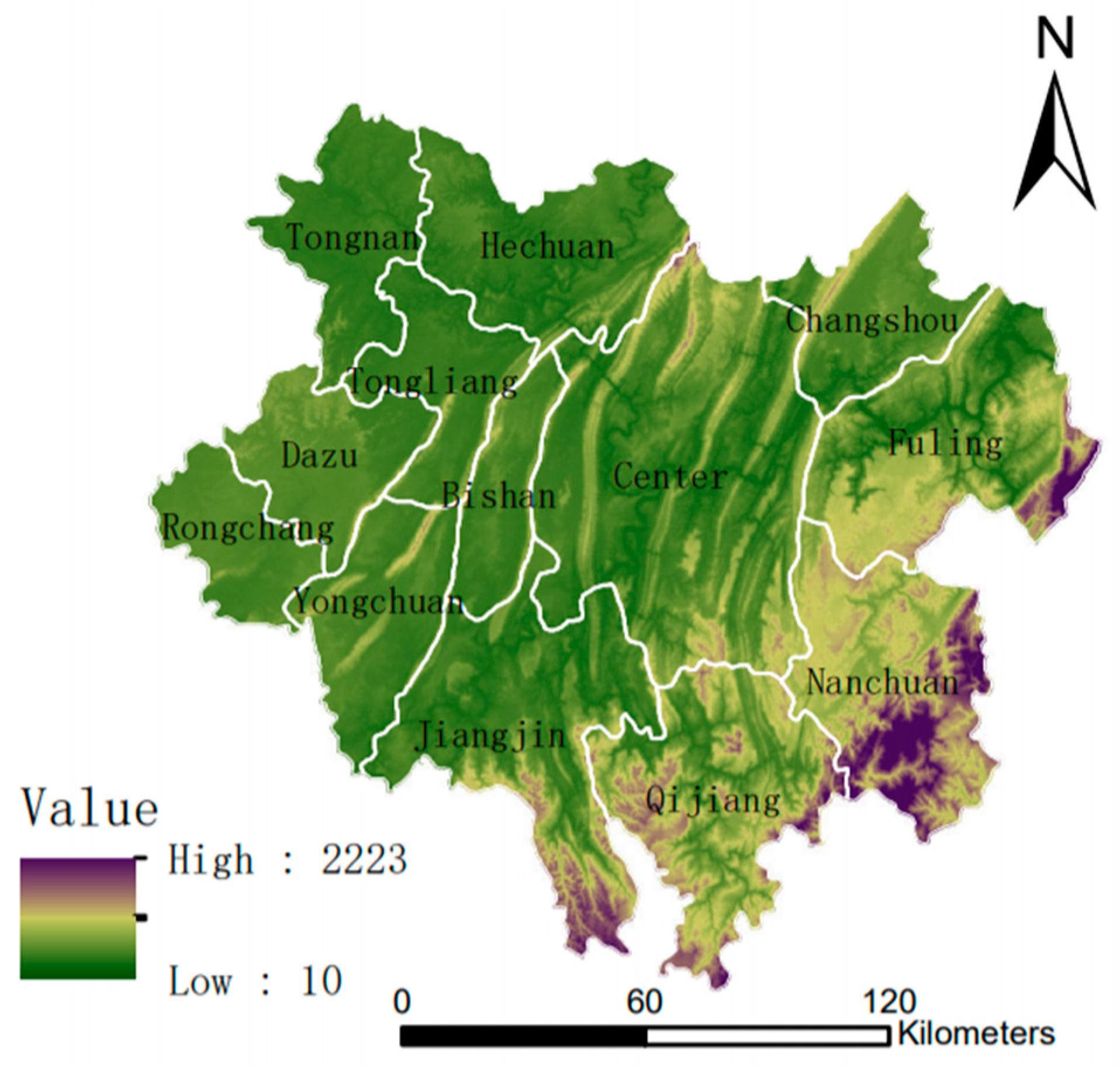
This study selects the urban area of Chongqing as the research region, encompassing the “Central Urban Area” and the “Main Urban New Area,” comprising a total of 21 districts (refer to Figure 1). Being the sole direct-controlled municipality in the western region, Chongqing is strategically located at the confluence of the central and western regions, as well as at the intersection of the Yangtze River Economic Belt and the Belt and Road Initiative, enjoying unique geographical advantages. Serving as a core part of the Chengdu-Chongqing economic zone, Chongqing plays a pivotal role as a key gateway, facing west and south towards the Eurasian continent. In recent years, Chongqing has strategically focused on the “Two Centers and Two Areas” (signifying important economic centers with nationwide influence, centers for technological innovation, areas for reform and opening-up, and high-quality living environments). This strategic positioning aims not only to promote the city’s internal development but also to vigorously propel the coordinated development plan within the Chengdu-Chongqing economic zone, marking a new strategic opportunity for Chongqing.
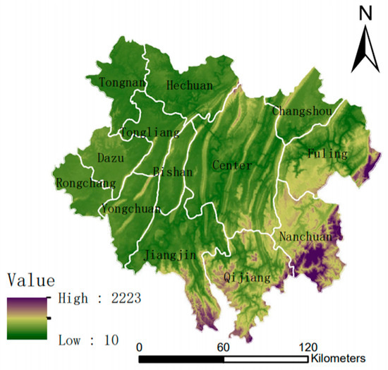
Figure 1.
Schematic diagram of Chongqing metropolitan area.
2.2. Data
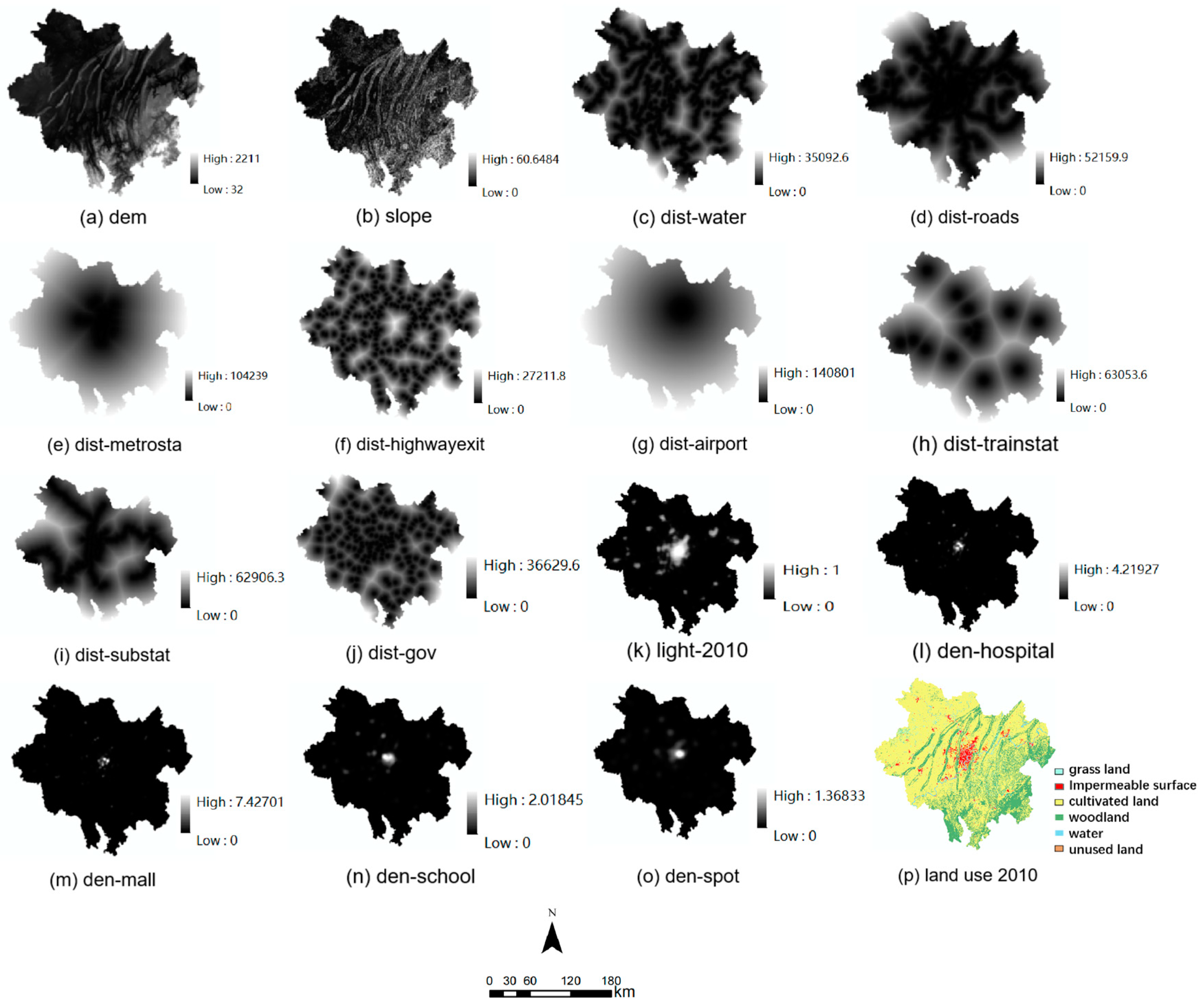
This paper selects urban expansion driving factor data from two perspectives: natural environment and socio-economic factors. The natural factors encompass elevation and slope data. The socio-economic factors include data such as hospital density, shopping center density, school density, tourist attraction density, nighttime light intensity, and accessibility factors like distances to the airport, town center, bus station, subway station, train station, railway, highway, and water bodies. The research data (Table 1) for land use originates from the Global Land Cover High-Resolution Observation and Monitoring (FROM-GLC) dataset with a resolution of 30 m. Based on Chongqing’s land use characteristics, the land use data was categorized into six types: grassland, impermeable surface, cultivated land, woodland, water bodies, and unused land. The heterogeneous data underwent the following procedures: (1) standardizing the research area, spatial coordinate system, and resolution (100 m); (2) conducting Euclidean distance calculations on water bodies and road networks using ArcMap 10.7 software; (3) calculating point density for point-of-interest data. Eventually, a unified dataset for driving factors and land use change was created (see Figure 2).

Table 1.
Data used in the study.
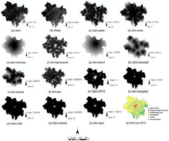
Figure 2.
Driving factors of 21 districts in Chongqing city.
2.3. Methods
The model mainly comprises four modules (see Figure 3): (1) Spatial Anisotropy Extraction Analysis Module; (2) Neighborhood Probability Extraction Module based on the Expansion Neighborhood-CNN Model; (3) Cellular Automata (CA) Dynamic Iteration Module based on the Inter-city Gravity Model; (4) Model Validation Module.
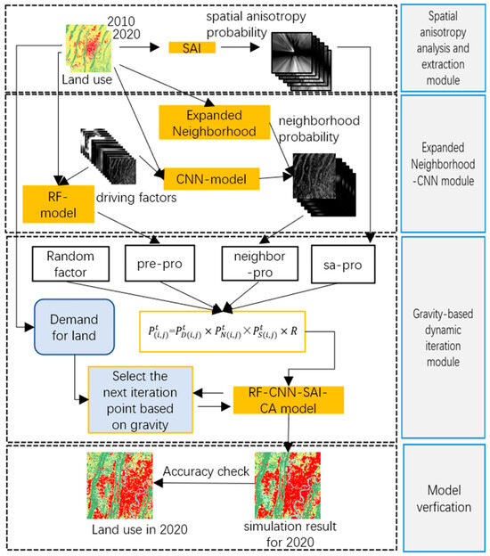
Figure 3.
Module flow chart.
The comprehensive transformation probability of a specific land-use class for each cell in the traditional Cellular Automata (CA) model depends on the land development suitability probability, neighborhood effect probability, constraint factors, and random effects.
In this article, to explore the impact of cell development in different spatial directions on land use change, we introduced the Spatial Anisotropy Index (SAI) into the traditional comprehensive transformation suitability module. The formula is as follows:
where, represents the comprehensive conversion probability of the cell at position ; denotes the urban development suitability probability of the cell at position , which in this paper is computed using the Random Forest (RF) module. It integrates 15 driver factor layers’ data with the land-use data changing from 2010 to 2020, establishing a unified spatial database. This suitability probability is derived by employing a random forest model based on the influencing driver factors. signifies the neighborhood effect probability of the cell at position , calculated in this paper by the expansion neighborhood and CNN module. stands for the Spatial Anisotropy Index (SAI) of the cell at position , representing the influence of forces from different directions on land-use change. represents the random effect during the land expansion and change process.
2.3.1. Spatial Anisotropy Module
Spatial Anisotropy (SA) is a significant feature in urban development, primarily focusing on the extent to which spatial directionality influences simulation results in urban expansion modeling. Specifically, it describes how different directions of urban expansion affect simulation results. For instance, in simulations, there may be variations in the evolution and changes of a non-urban cell in different spatial directions. In urban expansion modeling, partitioning schemes are commonly employed to address this directional issue, but this approach may lead to imbalances in simulation results in transition zones between two sector regions.
To delve deeper into revealing the spatial anisotropic patterns in urban land expansion, this paper introduces Spatial Anisotropy Index (SAI) on the basis of traditional urban expansion models. SAI quantifies the anisotropic probability of cells and integrates it into the overall conversion probability of cells. This allows for a more accurate simulation of urban expansion changes and development trends in different directions, thereby enhancing the accuracy and interpretability of simulation results.
How to measure anisotropy is crucial in anisotropy modeling. In contrast to the urban center, the proportion of pixels of a certain land use type in different directions compared to the total number of pixels in that direction exhibits significant differences. We refer to this proportion as the anisotropy index of a certain land type, as specified in Formula (2).
- : The anisotropy index of a certain land type.
- : The number of cells of a certain type along the line connecting the central city cell and the observation point.
- : The total number of cells along the line connecting the central city cell and the observation point.
Specific Steps: (1) Load Land Use Layer Data: Load land use layer data for the years 2010–2020, ensuring correct data formatting and the availability of land use type information for each cell. (2) Select City Center Point: Choose the center point of the city within the land use data layer, which can be either the geographic center of the city or a representative location. (3) Establish Four Quadrants: Create four quadrants around the city center point, dividing them according to the positive and negative directions of spatial coordinate axes. (4) Determine Line Equations: For randomly selected cell points within each quadrant and the city center point, calculate the line equations connecting them. This can be achieved using methods like two-point form or slope-intercept form. (5) Calculate Spatial Anisotropy Index (SAI): Utilize the aforementioned line equations to compute the Spatial Anisotropy Index (SAI) for each research point based on the provided formula. This index reflects the trends and differences of cells in different directions.
In this study, the spatial anisotropy index (SAI) for six types of land use in Chongqing in 2010 was calculated based on Formula (2) and the land use data of Chongqing in 2010. The results are presented in Figure 4.
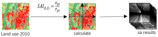
Figure 4.
SAI calculation process.
The spatial anisotropy index calculated earlier represents static observational (statistical) data at a specific point in time, which to some extent, expresses the directionality and preference of cell expansion in space. We believe that the factors leading to the anisotropic characteristics of land classes in spatial distribution stem from two forces: expansion forces from within the city (referred to as internal forces) and interactions between cities from outside (referred to as external forces). Presently, urban land change models place significant emphasis on internal forces but tend to overlook external forces due to several challenges in modeling them. In the CA iteration module of this study, we aim to explore the impact of external forces on urban expansion.
2.3.2. Neighborhood Effect Extraction Module
The traditional cellular neighborhood effect is a crucial mechanism used to describe the interaction between cells and how they respond to changes in the surrounding environment. Typically, the definition of neighborhood effect involves a fixed neighborhood structure that determines the surrounding neighboring cells considered by each cell. Taking the classic Moore neighborhood as an example, it includes eight adjacent cells around a cell. The fundamental idea of neighborhood effect is that the state update of a cell is influenced by the states of its neighboring cells, simulating local interactions between cells. However, traditional neighborhood effect methods have some limitations in certain situations. Firstly, they often employ a fixed neighborhood structure, which may limit the adaptability of the model, as some problems may require a more flexible neighborhood definition to better capture changes in the surrounding environment. Secondly, traditional neighborhood effect methods usually focus on the local neighborhood of cells, neglecting the influence of cells at greater distances on the simulation. This may lead to the model being unable to accurately predict global phenomena in some cases. Another limitation is that neighborhood effects may result in zero probabilities for some cell neighborhoods. This implies that, in certain situations, the state of a cell cannot change according to the current rules, leading to the abandonment of some cells with development potential and potentially inaccurate simulation results. In summary, although traditional neighborhood effects play a crucial role in cellular automaton models, they have some shortcomings in terms of flexibility, globality, and dynamics, which may limit the accuracy and applicability of the model.
Taking the neighborhood calculation of urban land as an example, the traditional mathematical expression of neighborhood calculation is: the density of urban cells within the neighborhood of the central cell. The mathematical expression of the neighborhood effect of cell at time is:
In the formula, is the neighborhood effect of cell at time , is the Moore neighborhood side length, con(.) is the conditional function, the value is 1 when the cell state is city, otherwise the value is 0, is the state of cell at time .
This article addresses the limitations of traditional neighborhoods in terms of flexibility, globality, and dynamics, particularly focusing on the issue of cell expansion failure in traditional neighborhood effect computations. It introduces the concept of an expanded neighborhood construction. The basic approach involves gradually increasing the side length of the neighborhood from 3, extending up to a maximum value of N (in this paper, through experimentation, N is chosen as 11), ensuring computational effectiveness and efficiency (refer to Figure 5). If the expansion up to N still fails to obtain effective neighborhood probability values, a Convolutional Neural Network (CNN) is utilized to extract spatial features from the perspective of the driving factors, further resolving the neighborhood effect.
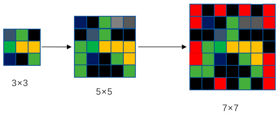
Figure 5.
Dynamic neighborhood expansion graph.
The yellow color in Figure 5 represents woodland, green denotes grassland, gray indicates arable land, black represents water bodies, red denotes built-up areas, and dark blue stands for unused land. In the first 3 × 3 Moore neighborhood, the calculated neighborhood effect for built-up areas is 0. When the Moore neighborhood expands to 5 × 5, the neighborhood effect for built-up areas remains 0. However, as the Moore neighborhood expands to 7 × 7, the neighborhood effect probability for built-up areas becomes 12/49. The concept of expanded neighborhoods proposed in this paper aims to address situations where there is a developmental trend, but the fixed neighborhood constraints lead to a neighborhood effect probability of 0 for cell points. Starting with the 3 × 3 Moore neighborhood is because this traditional neighborhood effect focuses more on the spatial correlation and explores the interaction between adjacent areas, capturing the characteristics and changes in local land use.
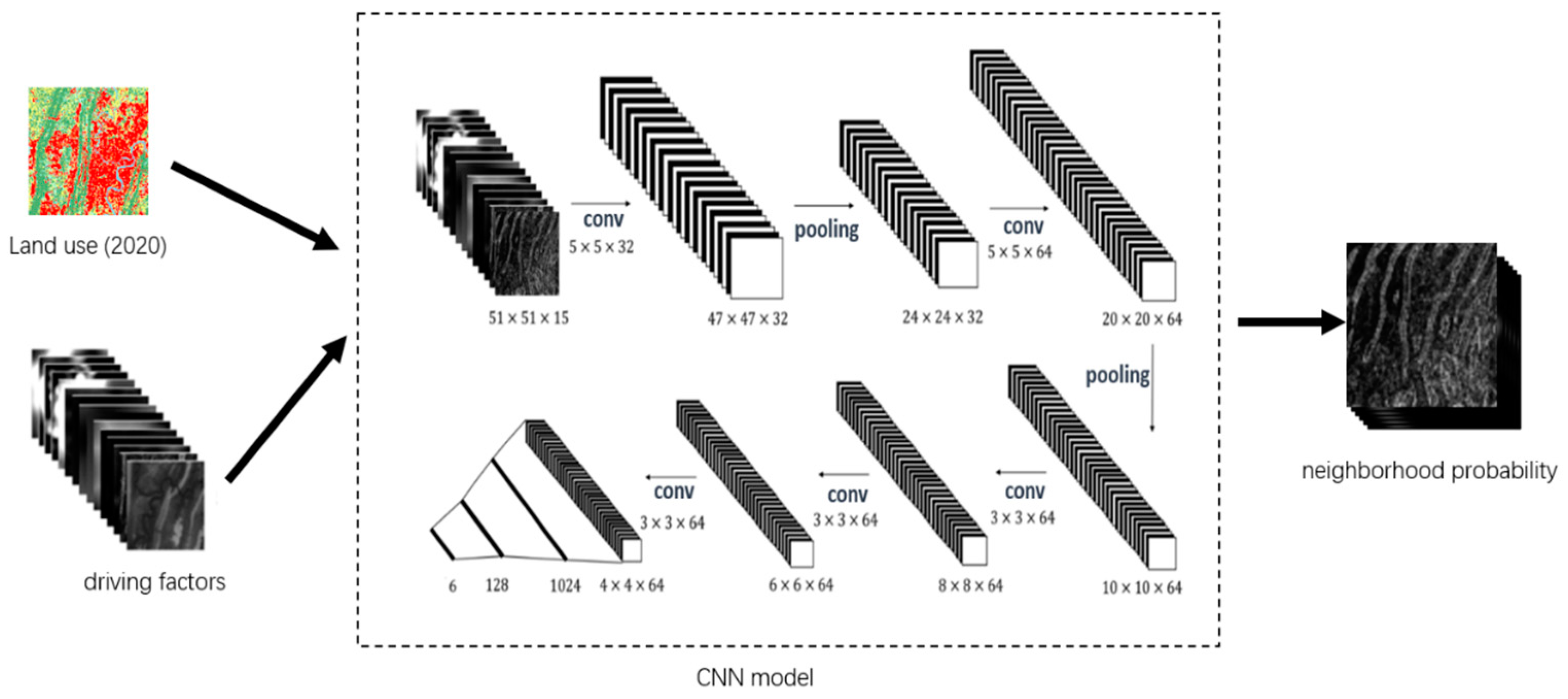
The traditional neighborhood calculation method, employing statistical techniques, is suitable for the spread and expansion of old areas but becomes ineffective in expressing the expansion of new areas. This is because, with the traditional method, there are cases where the probability is 0. If the traditional neighborhood calculation method continues, it objectively results in a lack of seed points for the expansion of new areas. Although expanded neighborhoods can reduce the occurrence of probability being 0 to some extent, it cannot completely eliminate this phenomenon. To address this issue, this paper introduces an alternative approach by leveraging convolutional neural networks (CNN) to extract the neighborhood effect at the driver factor level (see Figure 6). This is because the driver factors surrounding the cell’s neighboring points, to some extent, can also reflect the transformation trend of that cell point.

Figure 6.
Convolutional neural network model architecture diagram.
The first step involves preprocessing the land-use data for the year 2020 to obtain the dataset. Subsequently, with each label sample as the center, the neighborhood was established with a range set to N. This procedure led to the segmentation of the 15 driver factor layers into images of size N × N. According to the research of He Jialv, and considering the practical research conducted in this paper [8], the optimal value for N was found to be 51 for the model’s accuracy. Therefore, N was set to 51 in this study. Following this, the 51 × 51 × 15 image data was fed into the CNN model, undergoing convolution and pooling operations to ultimately output the neighborhood effect of the cell.
The CNN model mainly consists of 5 convolutional layers, 2 pooling layers and 2 fully connected layers. The activation function uses ReLu, the loss function uses CrossEntropy, and the stochastic gradient descent method is used during the training process.
2.3.3. CA Dynamic Iteration Module Based on Urban Inter-City Gravity Model
- (1)
- Comprehensive Suitability Extraction
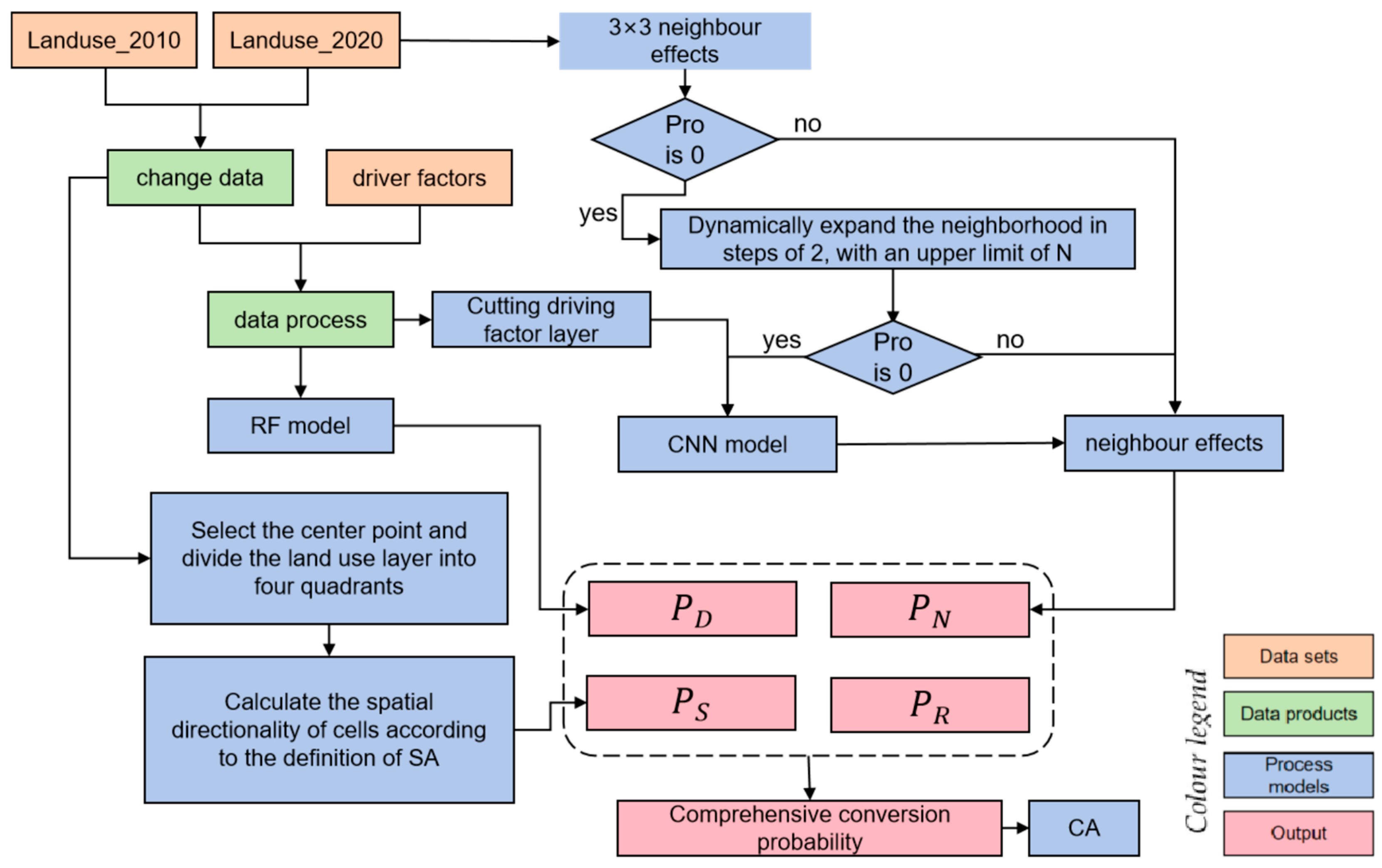
The operational process of the RF-CNN-SAI-CA model (Figure 7) is as follows: (1) Urban land use change data were obtained by detecting changes in land use classification data in the two periods before and after. After unifying the spatial reference system and resolution with the 15 driving factor layer data, a spatial database of dependent variables and independent variables in the study area was established; (2) To conduct stratified random sampling on a preprocessed unified dataset, the following steps are undertaken: Initially, label data for six types of land within the study area are quantified, resulting in 1,844,778 instances of label 1, 552,571 of label 2, 216,804 of label 3, 65,238 of label 4, 193,713 of label 5, and 40 of label 6. Subsequently, a random selection of 70% from each label category is extracted to form the training and testing dataset: 1,200,000 from label 1, 380,000 from label 2, 150,000 from label 3, 40,000 from label 4, 130,000 from label 5, and 30 from label 6. These datasets are then amalgamated and shuffled to create a comprehensive dataset containing 1,900,030 instances across six land use types. This dataset is further segmented into a training set, constituting 70%, and a testing set, accounting for 30%. Ultimately, this dataset is fed into a random forest model for training and testing. Subsequently, the comprehensive land use data from 2010 were applied to the trained RF model to obtain the initial conversion probability (urban development suitability) for each cell; (3) Subsequently, the neighborhood effect was determined based on the expansion neighborhood algorithm. If the neighborhood boundary expands to 11 × 11 and the probability remains zero, the next step involves training a Convolutional Neural Network (CNN) model using the preprocessed driving factor data. Based on the trained CNN model combined with the comprehensive driving factor dataset, the neighborhood effect probability based on the driving factors for the cells can be obtained; (4) According to the formula for Spatial Anisotropy Index (SAI) calculation, the spatial anisotropy probability for each cell point is computed; (5) According to the preliminary urban conversion probability, neighborhood effects, spatial anisotropy, and random factors, the overall transformation probability is calculated; (6) Using ARCGIS to calculate the total urban expansion based on land use data from 2010 and 2020, serving as the global constraint condition for the Cellular Automata (CA) model; (7) Incorporating the overall transformation probability into the CA model, selecting the next cell in the neighborhood based on the gravity model, iterating continuously to eventually obtain the simulation results.
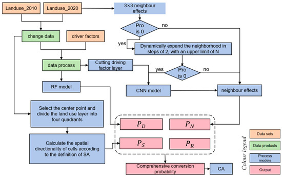
Figure 7.
RF-CNN-SAI-CA model structure.
- (2)
- Gravity-Guided Iteration Module
Another method introduced in this article is the gravity model to determine the magnitude of attraction between cities, assisting in analyzing the impact of intercity attraction on urban expansion. The formula is as follows:
Among them: is the attractiveness of city to city ; is the distance from city to city ; represents the quality of city , represents the quality of city ; are coefficients, Delphi method Determine: (The Delphi method is a technique for expert surveys, typically achieving consensus through iterative rounds of opinion collection and feedback. In this context, the Delphi method is employed to determine the coefficient values in the gravity model). For the gravity model formula between two cities, it can be written directly as .
Urban quality indicators: Urban quality indicators refer to indicators that can reflect the comprehensive strength of a city, or can reflect the comprehensive energy indicators of a city. In urban socio-economic development, four indicators, including population, gross regional product, total retail sales of consumer goods, and total import and export, are significant criteria for judging whether a city is developed. The urban quality index can be expressed as:
Among them, is the quality of the city, is the regional GDP, is the population, is the total retail sales of consumer goods, and is the total import and export volume.
Distance indicators involve geographical distance as well as subjective factors such as social, psychological, political, and cultural aspects. However, due to the difficulty in measuring subjective factors like social, psychological, political, and cultural distances, this paper employs geographical distance indicators to measure distances between cities. This choice is made because geographical distance is a relatively easy-to-measure objective indicator that can provide actual spatial gap information between cities, without being influenced by subjective factors.
Based on land transportation, this paper utilizes the geometric mean of three indicators—road distance, railway distance, and spatial latitude and longitude distance—to depict the distance between Chongqing and various cities, namely:
Among them, is the distance, is the highway mileage, is the railway mileage, and is the spatial longitude and latitude distance.
This article explores the 21 districts in the main city of Chongqing (Yuzhong District, Dadukou District, Jiangbei District, Shapingba District, Jiulongpo District, Nan’an District, Beibei District, Yubei District, Banan District, Fuling District, Changshou District, Jiangjin District, Hechuan District District, Yongchuan District, Nanchuan District, Qijiang District, Dazu District, Bishan District, Tongliang District, Tongnan District, Rongchang District) and the relationship between the development of the city and the gravitational force between cities, respectively, with the main city of Chongqing as the center point, from Qianjiang, Zunyi, Neijiang, Guang’an, Tongren, Luzhou, Chengdu and Dazhou were selected as research cities in 8 directions: east, south, west, north, southeast, southwest, northwest and northeast, and the 21 districts of Chongqing’s main city and 8 surrounding cities were explored gravitational relationship between them. Integrate gravity into the CA iteration module to create a CA dynamic iteration model based on gravity (Figure 8).
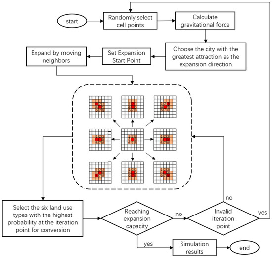
Figure 8.
CA model.
According to Formula (5), the comprehensive quality of each city is calculated (Table A1); based on Formula (6), the comprehensive distance from each research area in the main city of Chongqing to the surrounding cities is calculated (Table A2); using the data from Table A1 and Table A2 in conjunction with Formula (4), this paper computed the magnitude of gravitational pull between the 21 main districts of Chongqing and the surrounding 8 cities (refer to Table A3). To better analyze the impact of these gravitational values, we normalized these data. Normalization transforms the data into a distribution with a mean of 0 and a standard deviation of 1. In this paper, the gravitational value of cells at position concerning surrounding cities is denoted as , which is integrated into the overall conversion probability as follows: =×, where = (). It reflects the external directional probability brought by the size of gravitational forces, contributing to the external directionality of cells. It is worth noting that the computation parameters for gravitational size are related to the population and economic factors of construction land. Hence, this paper only introduces this module on simulating construction land (non-permeable surface) to explore the impact of gravitational forces from surrounding cities on the simulated urban development results.
The specific calculation process begins by using the ArcMap tool to process the administrative boundary vector map of the 21 main urban districts in Chongqing (Figure 9a). The vector map is converted into raster data by uniformly setting the resolution to 100. In this process, rasterization is performed based on the NAME attribute of the main urban districts, ensuring that each region has a unique corresponding label in the obtained raster data layer of the 21 main urban districts in Chongqing (Figure 9b), with labels ranging from 1 to 21. Next, based on the land-use data layer of the base year, a starting cell point is randomly selected, serving as the starting point for the Cellular Automaton (CA) dynamic simulation. Using this cell as the center, a 3 × 3 Moore neighborhood is constructed as the foundational structure for iteration. For each iteration, the corresponding region label for the current cell is identified by its coordinates in Figure 9b, thereby determining the specific area to which the cell belongs. Subsequently, using the precomputed area-specific gravitational values from Table A3, an assessment and comparison of the gravitational values for each direction within the 3 × 3 Moore neighborhood are performed (8 grid positions represent 8 directions). Among the gravitational values in the eight directions, the direction with the highest gravitational value is chosen as the target for the next iteration. Simultaneously, the probability of construction land at the selected iteration point is multiplied by , the specific land type conversion at that iteration point is jointly determined by the conversion probabilities of the other five land types and the enhanced probability of transforming into construction land. Among all possible land type conversions, the type with the highest probability is selected for conversion. After completing these steps, the count of this land type is incremented by 1, and the iteration continues. This process continues until the count of the six planned land use types for 2020 is reached. If the count of a certain land type reaches the planned value during the iteration, in the subsequent iterations, the comprehensive conversion probability of that land type will no longer be considered.
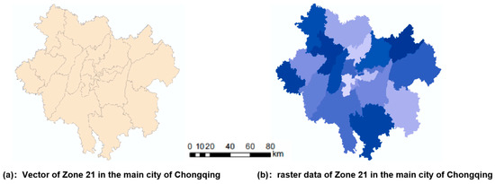
Figure 9.
Vector and raster data of Zone 21 in the main city of Chongqing.
In Figure 8, the red color represents seed cell elements, while the brown area represents the 3 × 3 Moore neighborhood constructed around the seed cell. The numbers 1–8 represent the magnitude of gravitational force between Chengdu, Guang’an, Dazhou, Neijiang, Qianjiang, Luzhou, Zunyi, and Tongren, respectively, and the central seed cell element. The point with the maximum gravitational force is chosen as the next iteration’s seed cell, and the overall transformation probability of the construction land type at this iteration point is multiplied by the normalized gravitational force value . Then, based on the overall conversion probability of the six land use types at that cell point, the conversion status of that cell is determined. The process continues by constructing a 3 × 3 Moore neighborhood for iteration until the land quantity reaches the land demand of the current year, at which point the iteration stops.
2.3.4. Model Validation Module
Overall Accuracy (OA) and Kappa coefficient are commonly used as metrics for model accuracy assessment. Overall Accuracy represents the ratio of correctly classified samples to the total number of samples in the simulation results, calculated by the formula:
- : The anisotropy index of a certain land type.
- A: The total number of samples or grid cells.
The Kappa coefficient is calculated based on the confusion matrix and is commonly used to measure classification accuracy and conduct consistency checks. The Kappa coefficient takes into account the possibility of chance agreement, making it more reliable than simple percentage calculations. The formula for calculating the Kappa coefficient is:
- : Kappa coefficient.
- : The sum of correctly classified samples for each class divided by the total number of samples, i.e., overall classification accuracy.
- : The sum of the products of actual and predicted quantities for each category, divided by the square of the total number of samples.
The value range of the Kappa coefficient is [−1, 1], and usually the value range of the actual result is [0, 1]. The closer the Kappa coefficient is to 1, the higher the consistency between the model simulation results and the actual results.
In actual urban expansion, the area of unchanged area is usually much larger than the area of changed area. R. G. Pontius [38] proposed the (Figure of Merit, FOM) based on the difference in changes between actual results and simulated results. Compared with OA and Kappa coefficient, FOM more accurately reflects the consistency and accuracy of simulation of complex geographical systems. FOM is calculated as follows:
A represents the number of grids that actually changed but were predicted as unchanged, B is the number of grids that actually changed and were predicted to change, C is the number of grids that actually changed but were incorrectly predicted in terms of land use category, and D is the number of grids that did not change but were predicted to change.
3. Results
3.1. Model Training and Prediction
3.1.1. Training Model and Key Steps
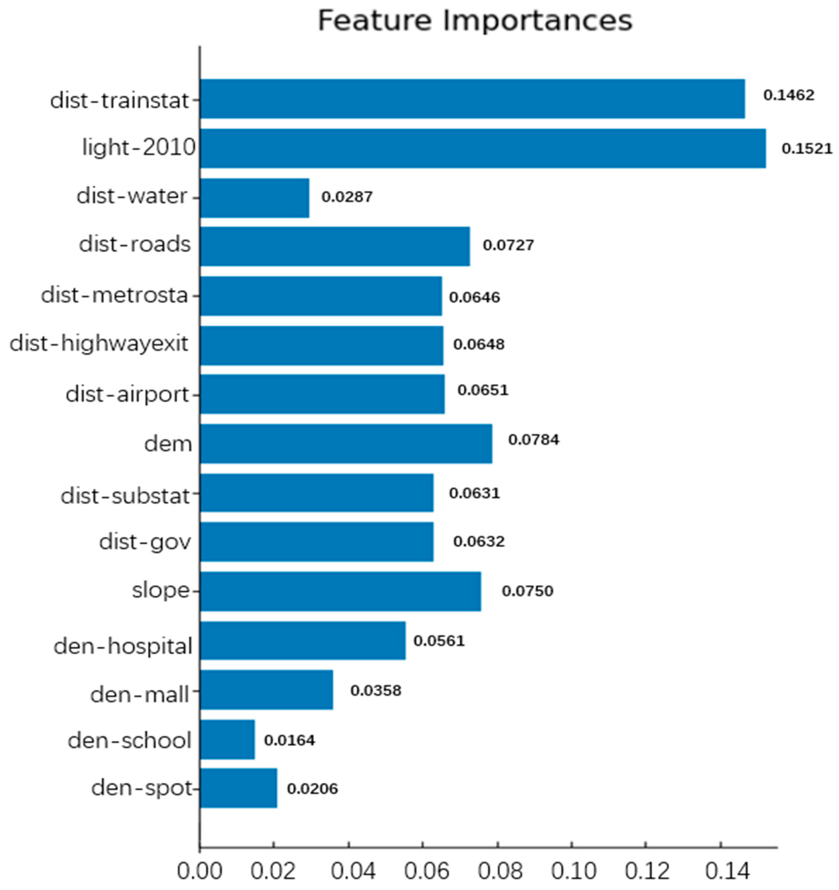
Enter the 15 driving factor layer data, use the 2010 and 2020 land use data through ARCGIS operations to obtain the changing land use data, merge the changing land use data and the 15 driving factor data, remove duplicates, and randomly sample. The sampled data was divided into a test set and a training set and fed into the random forest model for training and testing. The accuracy of the random forest was determined to be 0.9576, and the impact of each driving factor on urban expansion was obtained (Figure 10). Randomly select a cutting point on the 2010 layer, center the 15 driving factor layers on the coordinates of the cutting point, cut the matrix into a size of 51 × 51, and input the labels into the CNN model for iterative training. The accuracy obtained for the CNN model is 0.8677.

Figure 10.
Importance of driving factors.
Figure 10 shows the calculation results of the importance of driving factors. From the results, it can be seen that nighttime light data and distance from train station data have the greatest impact on urban expansion, which are 0.1521 and 0.1462, respectively. Distance to water bodies, school density, and attraction density data have a weak impact on urban expansion.
The maximum impact of nighttime lighting is likely due to the illumination reflecting the economic development, population density, and human activity intensity in the corresponding area. The primary driving force behind urban expansion is derived from these factors. The significant influence near a train station is probably because train stations typically serve as crucial hubs in urban transportation, with high population mobility and commercial activities in their vicinity, making them potential hotspots for urban expansion. This is related to the usual promotion of urban expansion through convenient transportation and economic activities. In contrast, the impact of proximity to water bodies and school density is relatively minor, possibly because these factors play a secondary role in urban expansion. Water bodies may be subject to restrictions in planning and environmental considerations, limiting urban expansion around them. School density may not be a primary driving factor in urban planning, as school distribution is typically influenced by educational planning and population density considerations. Overall, the magnitude of these factors’ impact may depend on the specific circumstances of urban planning, including urban development strategies and policy planning.
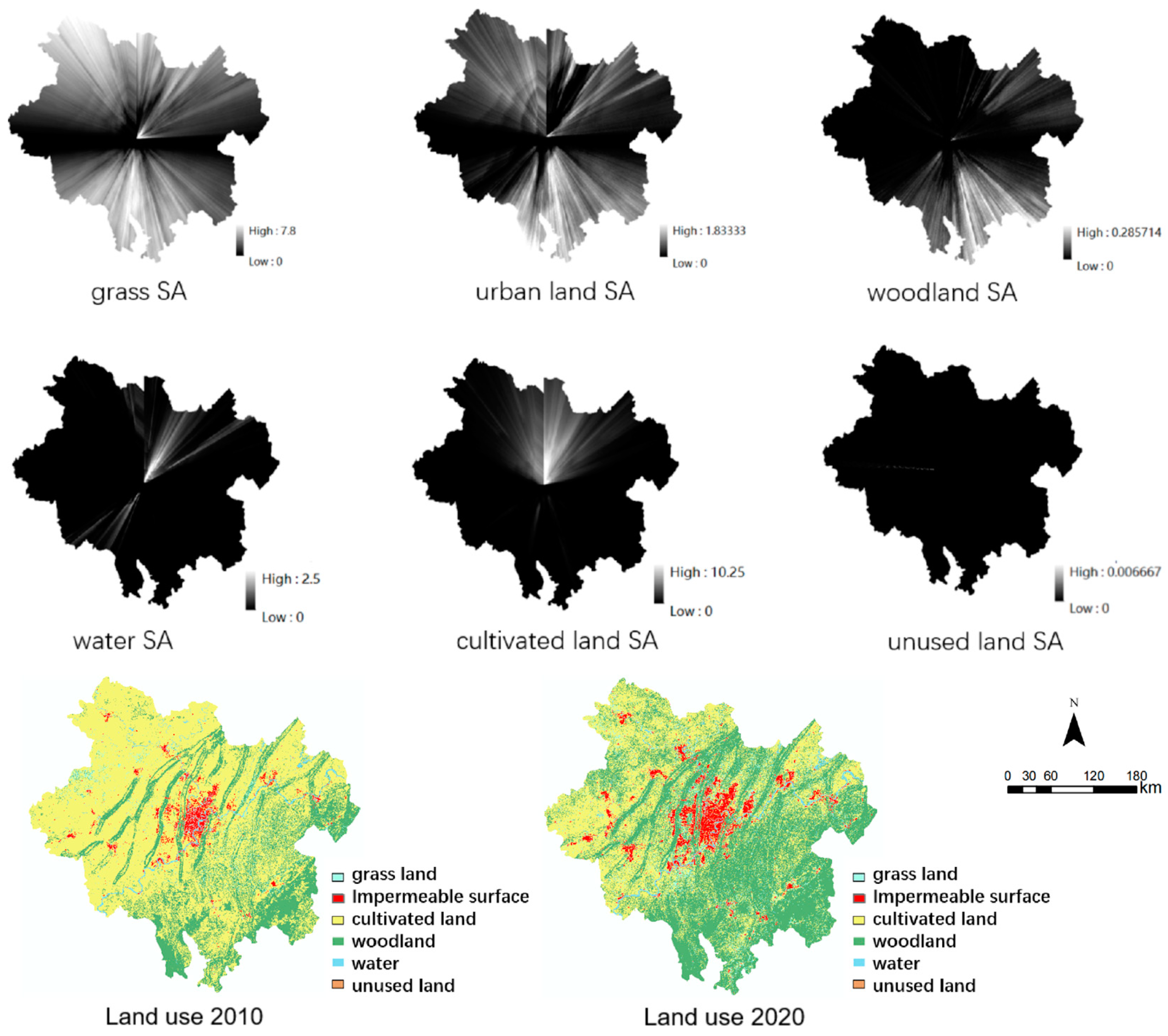
3.1.2. Analysis of Spatial Anisotropy Results
Algorithm 1 is the algorithm for calculating the spatial anisotropy index of cells whose label is 0, indicating the land type as grassland. Based on the algorithm provided in Algorithm 1, the spatial anisotropy probability layer for the remaining five land use types can be calculated similarly (as depicted in Figure 11). This study computes the spatial anisotropy probabilities for six land use categories using the 2010 land use data and incorporates them into the comprehensive transformation probability for forecasting land use changes in 2020. The visualization in Figure 11 indicates that grassland, construction land (impervious surface), forestland, and cultivated land exhibit stronger spatial anisotropy compared to water bodies and unused land (where darker colors represent weaker spatial anisotropy). Specifically, forestland tends to have stronger spatial anisotropy in the southeast direction, water bodies display stronger spatial anisotropy in the northeast direction, while cultivated land shows stronger spatial anisotropy in the north direction. Unused land, on the other hand, demonstrates weaker overall spatial anisotropy, primarily due to its smaller area coverage. As per the 2020 land use legend, the trends in the development of various land use types predicted by the spatial anisotropy module align well with the actual changes observed in 2020. Notably, the development trends for grassland and woodland exhibit the strongest correlation with the observed changes.
| Algorithm 1 Get spatial anisotropic probability layer pseudocode. |
| Input: 2010 land use raster data LandUse (2290 × 2438), coordinates of the first quadrant research point in point1.txt Output: SA_pro (spatial anisotropy probability) |
Process:
|

Figure 11.
SA of various land use types.
3.1.3. Expanded Neighborhood Result Analysis
In order to depict the impact of varied upper limits of the expanded neighborhood (N) on model accuracy more accurately, this paper examines the correlation between different upper limits of the expanded neighborhood and FOM (Figure 12). Within the range of 3 to 9 for the expanded neighborhood (N), there is a noticeable upward trend observed in FOM. At N = 11, FOM peaks at 0.4486, indicating the highest accuracy in model simulation. However, as N increases to 15, there’s a sharp decline in FOM. Further, within the range of 13 to 19, FOM generally demonstrates a downward trend. Consequently, this study opts for N = 11 as the upper limit for the expanded neighborhood, as it exhibits the highest model accuracy among the considered values.
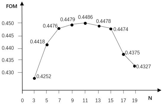
Figure 12.
Relationship between the upper limit N of the expanded neighborhood and FOM.
From Table 2, it is evident that the Kappa value of the RF-CNN-SAI-CA model derived from expanded neighborhoods is 0.8457, and the FOM stands at 0.4486. Comparatively, this FOM value is 0.0060 higher than the Kappa of the RF-CNN-SAI-CA model that was based on driving factors for assessing neighborhood effects. With an FOM exceeding 0.0055, it suggests that the neighborhood effect computed using expanded neighborhoods more accurately captures the pattern of urban expansion, thereby enhancing the model’s accuracy.
3.1.4. Analysis of Urban Gravity Results
According to Formula (5), the comprehensive quality of the 21 districts in Chongqing’s main city and the eight surrounding cities can be calculated (Table A1, see Appendix A).
According to Formula (6), the comprehensive distance between the 21 districts in Chongqing’s main city and the eight surrounding cities can be calculated (Table A2, see Appendix A).
According to Formula (4) and the data in Table A1 and Table A2, the mutual attraction size between the main urban area of Chongqing and the surrounding cities can be calculated (Table A3, see Appendix A). Incorporating the gravitational values from Table A3 into the CA dynamic iteration module, the impact of external urban attraction on the simulation of urban expansion is explored. From Table A3, it can be observed that Guang’an has a greater attraction size towards Yubei District and Hechuan District, while Luzhou has a stronger attraction size towards Yongchuan District compared to other areas in the main urban zone of Chongqing. Due to smaller urban qualities in Tongren and Qianjiang and larger comprehensive distances, the attraction towards the 21 districts of Chongqing’s main urban area is relatively smaller. The gravitational values in the table can reflect to some extent the development trends of various regions in the main urban area of Chongqing.
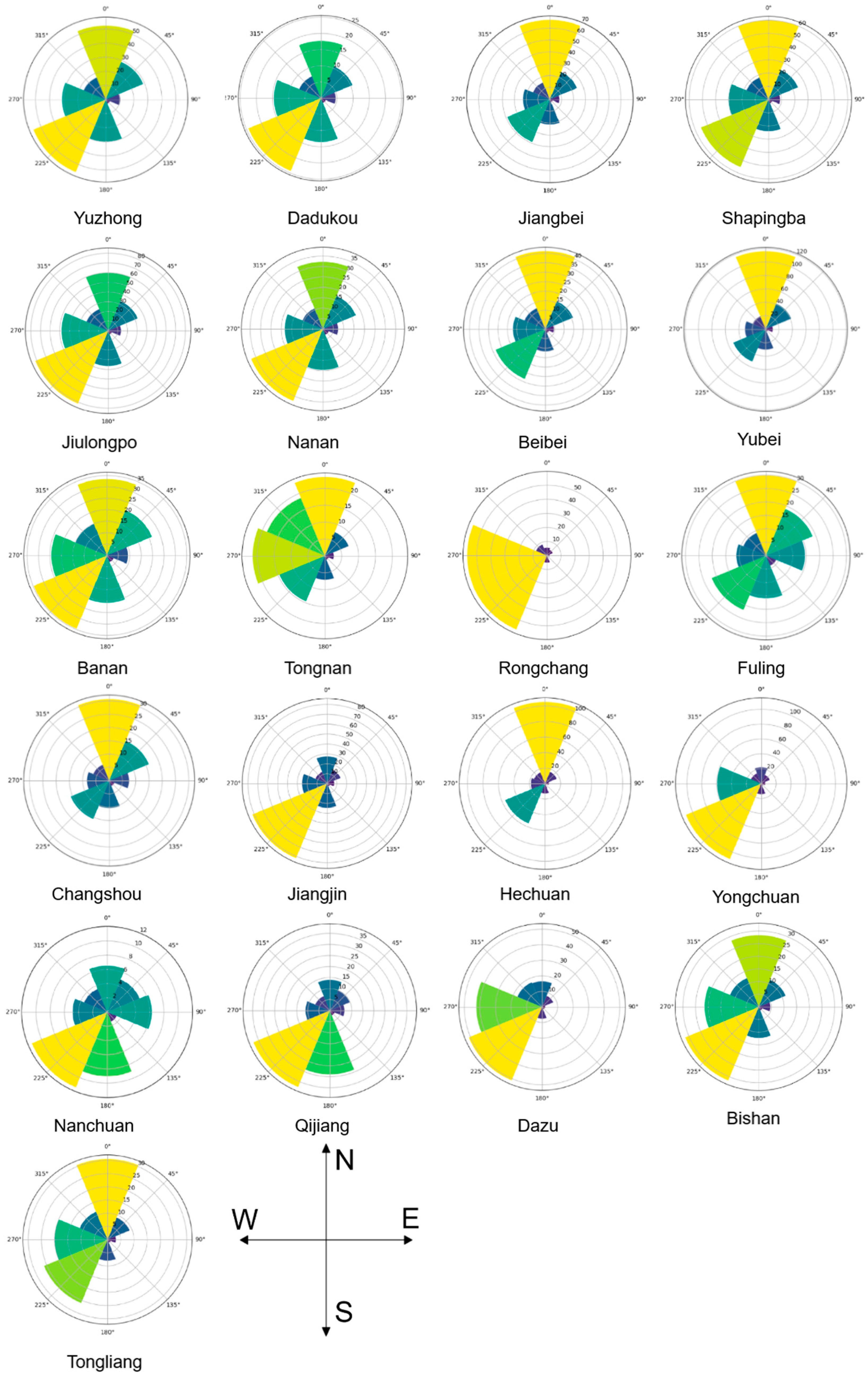
By analyzing and visualizing the data in Table A3, Figure 13 has been obtained, which clearly illustrates the magnitude of gravitational strength between the main urban area of Chongqing (21 districts) and the surrounding eight cities. Taking Yuzhong District as an example, Figure 13 depicts its gravitational strength distribution in different directions. It shows that the greatest gravitational strength exists in the north and southwest directions, while the weakest gravitational strength is in the east and southeast directions.
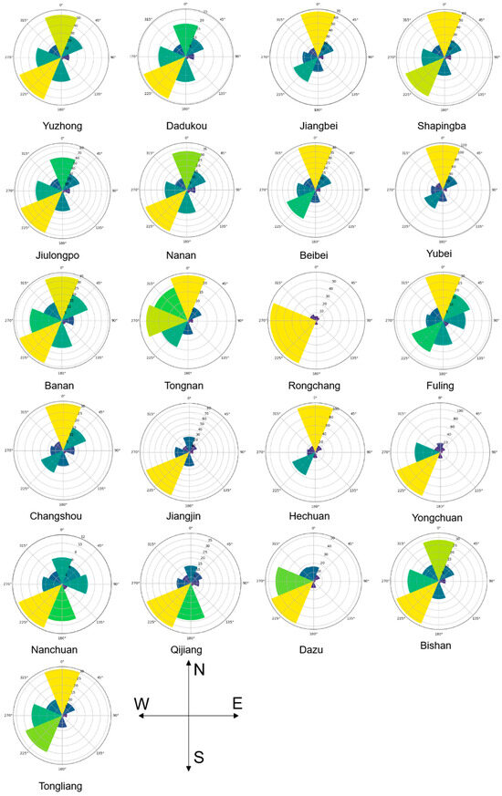
Figure 13.
Visualization of the gravity of Chongqing district 21 and eight surrounding cities.
To further explore the impact of integrating the gravity model on simulating construction land, this study conducted experimental comparisons by calculating the F1-score of construction land simulation before and after integrating the gravity model, resulting in 0.8932 and 0.9317, respectively. The experimental results indicate that integrating the gravity model significantly enhances the accuracy of construction land simulation, thereby improving the overall model precision. This enhancement might stem from the gravity model’s consideration of various factors such as economy, population, and spatial distance in predicting future development trends of construction land. Consequently, cells with the highest gravity values have a higher probability of transformation, thus improving the simulation accuracy.
3.1.5. Model Simulation Results
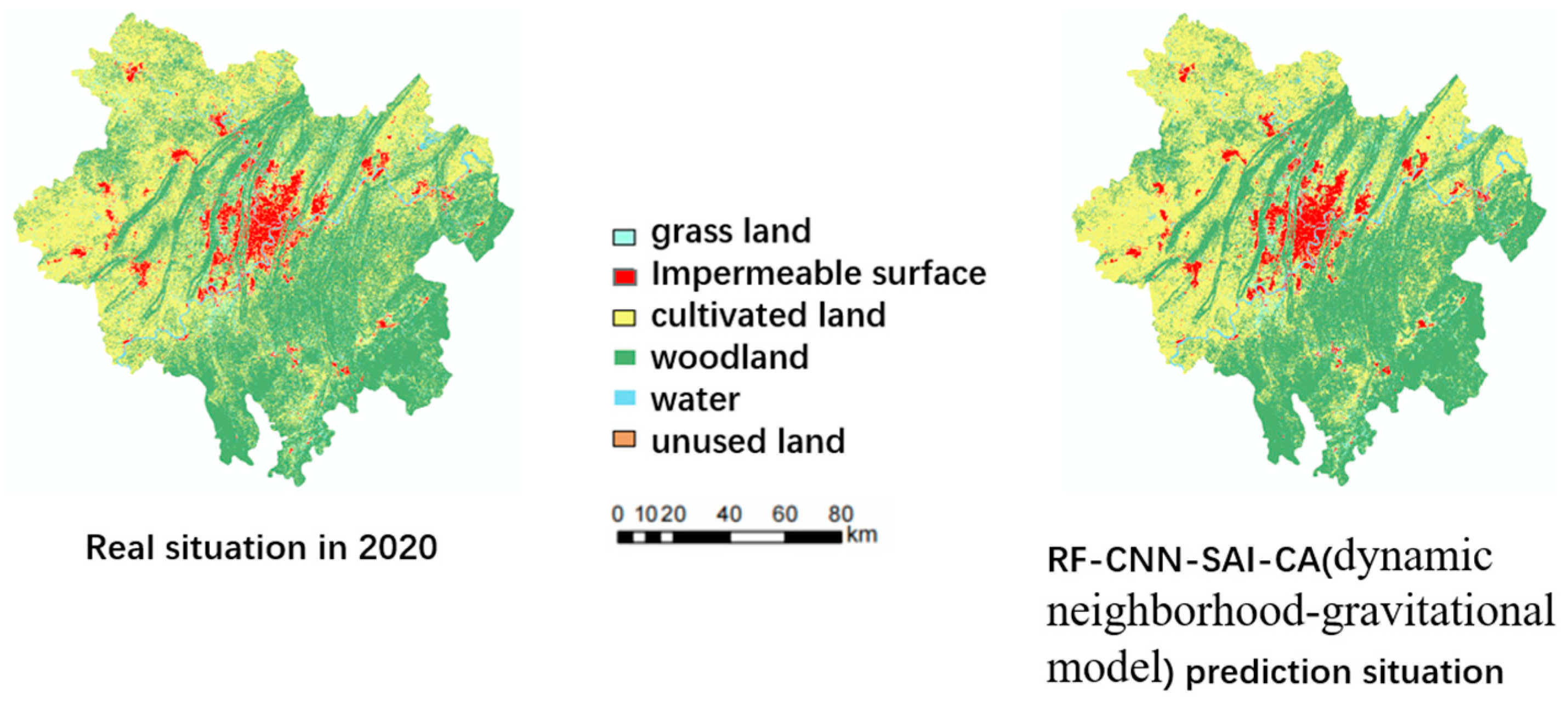
The RF-CNN-SAI module, combined with random factors, generated the overall transformation probability layer. Subsequently, based on the change data, the global expansion total constraint conditions were calculated. Then, the gravity formula was applied to the final Cellular Automata (CA) model for CA dynamic simulation. This process yielded the comparison between the simulated 2020 urban expansion results (initiated with Chongqing’s main city data from 2010) and the actual 2020 results (Figure 14). Table 2 and Table 3 demonstrate that considering both the spatial anisotropy within urban cells and the mutual gravity between cities improves the precision of urban expansion simulation.

Figure 14.
Comparison between 2020 real situation and prediction.
3.2. Simulation Result Evaluation
Accuracy Comparison
To further verify the reliability and efficiency of the experimental results in this paper, a series of ablation experiments were designed. The results of these experiments are shown in Table 2. Additionally, a series of comparative experiments were conducted, with the results presented in Table 3.
Table 2.
Ablation experiment of simulation accuracy.
Table 2.
Ablation experiment of simulation accuracy.
| Parameter | RF-CNN-SAI-CA (Dynamic Neighborhood-Gravitational Model) | RF-CNN-SAI-CA (Dynamic Neighborhood) | RF-CNN-SAI-CA |
|---|---|---|---|
| Kappa | 0.8561 | 0.8457 | 0.8397 |
| FOM | 0.4596 | 0.4486 | 0.4431 |
| OA | 0.9896 | 0.9862 | 0.9798 |
Table 3.
Comparison of simulation accuracy.
Table 3.
Comparison of simulation accuracy.
| Parameter | RF-CNN-CA | RF-CA | FA-MLP-CA | RF-SNSCNN-CA |
|---|---|---|---|---|
| Kappa | 0.8376 | 0.8154 | 0.6984 | 0.7683 |
| FOM | 0.4322 | 0.4067 | 0.3942 | 0.3836 |
| OA | 0.9766 | 0.9742 | 0.9789 | 0.9782 |
4. Discussion
According to the ablation experiment in Table 2, it can be seen that the Kappa and FOM of the RF-CNN-SAI-CA model based on gravity and expanded neighborhoods are improved by 0.0104 and 0.0110, respectively, compared with the RF-CNN-SAI-CA model based on expanded neighborhoods. Considering the gravitational relationship between cities in the basic model of this article is helpful to explore the intrinsic mechanism of urban expansion. According to Table 3, The RF-CNN-SAI-CA model, based on expanded neighborhoods, has shown an improvement in Kappa, FOM, and OA coefficients by 0.0303, 0.0419, and 0.0120, respectively, compared to the traditional RF-CA model, demonstrating that incorporating spatial anisotropy and expanding the neighborhood effectively enhances the model’s simulation accuracy. To further validate the model’s accuracy, this article’s RF-CNN-SAI-CA model, based on the expanded neighborhood, is compared with RF-CNN-SAI-CA, RF-CNN-CA, and FA-MLP-CA models. The first two models aim to mitigate the impact of expanded neighborhoods and spatial anisotropy. Results indicate that the Kappa, FOM, and OA values of this model surpass those of the other two models. The Kappa coefficients have improved by 0.0060 and 0.0081, respectively, and FOM has increased by 0.0055 and 0.0164. The third model represents an alternative solution to address spatial directionality. The outcomes reveal that this model’s accuracy is superior, highlighting that the RF-CNN-SAI-CA model, utilizing expanded neighborhoods, is more conducive to exploring rules governing urban expansion. The fourth RF-SNSCNN-CA model is a relatively new urban expansion simulation model. According to experimental results, it can be observed that the accuracy of the proposed model in this paper is higher, further highlighting the advantages of the model proposed in this study.
Investigating the influence of spatial directionality on urban expansion simulation, this study focuses on Chongqing’s main urban area, constructing an RF-CNN-SAI-CA model grounded on expanded neighborhoods and gravitational effects. The model comprises four modules. The initial module utilizes the robustness of random forest to compute urban suitability probabilities based on driving factors, establishing preliminary conversion probabilities. The second module addresses neighborhood effects, proposing a model combining expanded neighborhoods and CNN for handling cell neighborhood limitations. The third module supplements traditional overall conversion probabilities with cell directional probabilities, and the fourth module introduces the gravity formula into Cellular Automata (CA) simulation to explore inter-city gravitational impacts on urban expansion. Additionally, this paper conducts comparative analyses with other models. Table 2 and Table 3 illustrate that the simulation accuracy of the RF-CNN-SAI-CA model, based on gravity and expanding neighborhood, is slightly higher than that of other models. This constructed model not only enhances the accuracy of land use change simulation to a certain extent but also introduces a novel approach for studying similar spatiotemporal simulation issues. The key conclusions drawn in this study are as follows:
- (1)
- The conventional urban expansion simulations often lack the probability trend of cells converting to specific land use types in particular directions, resulting in inaccurate simulation outcomes. This paper successfully enhances the precision of urban expansion simulation by introducing Cellular Directional Probability (SAI). This innovative approach allows the model to more accurately mirror the genuine patterns of urban expansion and offers fresh insights into analogous spatiotemporal simulation issues.
- (2)
- In addition to accounting for directional probability within the city, this study also incorporates the gravity model formula to investigate the influence of intercity attraction on urban expansion simulation. Through an analysis of the gravitational relationship between Chongqing and eight surrounding cities, this research reveals that the urban expansion process is impacted not solely by internal factors but also by the mutual attraction among cities. This discovery underscores the significance of intercity interactions in urban expansion simulations.
- (3)
- Neighborhood effects are crucial considerations in urban expansion simulations. However, traditional methods face an issue of cellular neighborhood failure. To address this problem, this paper proposes a solution by integrating the expanded neighborhood and a CNN-based neighborhood effect model. Through this innovative approach, this paper successfully enhanced simulation accuracy, effectively remedying the issue of cell loss in the neighborhood effect, thus rendering the simulation results more precise.
The study of urban expansion plays a crucial role in modern urban planning and land use decisions, as it pertains to the future sustainable development of cities. However, prior research on simulating urban expansion has had some limitations, including overlooking the directional trend of cell land use changes, neglecting intercity mutual attraction, and encountering issues with cell loss in neighborhood effects. This paper introduces the RF-CNN-SAI-CA model based on gravity and expanded neighborhoods, marking significant advancements in urban expansion simulation. By incorporating cell directional probability and expanded neighborhoods, this model enhances simulation accuracy and addresses prior research gaps. Nevertheless, there remain areas for further enhancement within this model. One critical aspect is the model’s lack of consideration for the influence of government factors on urban expansion. Government policies and planning significantly shape a city’s land use and development trajectory. Future research could involve integrating government policy factors into the model to achieve more precise urban expansion simulations. Additionally, in the gravity module, this study only selected eight cities around Chongqing as research objects. However, urban development is generally influenced by the interaction forces among cities over a broader geographical area. The development of Chongqing may also be influenced by urban clusters formed by the interaction forces among other cities. Still, this paper only considered the forces between Chongqing and each individual city. Future research could consider expanding the study scope, incorporating more potentially interrelated cities, to gain a more comprehensive understanding of the dynamic processes of urban expansion. The challenge faced by the SAI index module lies in its dependence on linear equations to count the number of cells on the corresponding line. In experiments, situations where the slope of the line is zero led to equation failure, causing the SAI index values for certain points to become ineffective, thereby affecting the accuracy and precision of the simulation results. In the future, the model can be further refined to achieve more accurate and detailed simulations of urban expansion, providing more forward-looking support for urban planning and land-use decision-making. This would aid in promoting sustainable urban development and addressing the increasing needs of urban populations and resource utilization.
Author Contributions
Conceptualization, Minghao Liu and Jianxiang Wang; methodology, Jianxiang Wang; software, Jianxiang Wang and Qingxi Luo; validation, Minghao Liu and Lingbo Sun; formal analysis, Minghao Liu and Jianxiang Wang; investigation, Jianxiang Wang and Enming Wang; resources, Minghao Liu; data curation, Jianxiang Wang; writing—original draft preparation, Jianxiang Wang; writing—review and editing, Minghao Liu and Qingxi Luo; visualization, Jianxiang Wang; supervision, Minghao Liu; project administration, Chun Chen; funding acquisition, Chun Chen. All authors have read and agreed to the published version of the manuscript.
Funding
This research was funded by National Natural Science Foundation of China, grant number 42071218.
Data Availability Statement
The datasets presented in this article are not readily available because the data and code were processed in a local environment, and some of the data was acquired through purchase. Requests to access the datasets should be directed to liumh@cqupt.edu.cn.
Acknowledgments
We thank Chen Chun for funding acquisition and project administration.
Conflicts of Interest
The authors declare no conflicts of interest.
Appendix A
Table A1.
Comprehensive quality of the Chongqing region and surrounding cities.
Table A1.
Comprehensive quality of the Chongqing region and surrounding cities.
| Area | Quality | Area | Quality | Cities | Quality |
|---|---|---|---|---|---|
| Yuzhong | 754.46 | Fuling | 640.81 | Chengdu | 2226.51 |
| Dadukou | 324.54 | Changshou | 394.89 | Guangan | 1466.94 |
| Jiangbei | 599.88 | Jiangjin | 573.23 | Dazhou | 2002.38 |
| Shapingba | 664.42 | Hechuan | 538.25 | Luzhou | 2159.32 |
| Jiulongpo | 952.44 | Yongchuan | 556.59 | Zunyi | 2229.54 |
| Nanan | 503.21 | Nanchuan | 229.28 | Neijiang | 1337.84 |
| Beibei | 426.18 | Qijiang | 428.95 | Tongren | 1203.35 |
| Yubei | 902.79 | Dazu | 374.76 | Qianjiang | 1053.71 |
| Banan | 618.84 | Bishan | 399.94 | ||
| Tongnan | 366.43 | Tongliang | 334.21 | ||
| Rongchang | 245.75 |
Table A2.
Comprehensive distance from the Chongqing main region to surrounding cities.
Table A2.
Comprehensive distance from the Chongqing main region to surrounding cities.
| City | Chengdu | Guangan | Dazhou | Luzhou | Zunyi | Neijiang | Tongren | Qianjiang |
|---|---|---|---|---|---|---|---|---|
| Yuzhong | 315.05 | 145.22 | 228.87 | 170.90 | 237.60 | 180.10 | 534.88 | 277.25 |
| Dadukou | 314.97 | 164.04 | 247.69 | 169.64 | 231.28 | 172.60 | 496.67 | 272.71 |
| Jiangbei | 294.50 | 114.60 | 220.10 | 182.59 | 250.60 | 188.28 | 538.93 | 281.53 |
| Shapingba | 286.50 | 127.50 | 234.76 | 161.10 | 248.30 | 171.21 | 506.49 | 281.17 |
| Jiulongpo | 295.90 | 152.82 | 240.17 | 158.80 | 241.30 | 162.60 | 529.59 | 274.20 |
| Nanan | 324.40 | 151.27 | 242.70 | 170.50 | 239.20 | 191.52 | 450.10 | 269.95 |
| Beibei | 282.42 | 123.24 | 231.91 | 180.20 | 284.71 | 183.00 | 495.62 | 316.70 |
| Yubei | 310.60 | 106.80 | 209.50 | 193.61 | 257.59 | 198.52 | 554.91 | 297.71 |
| Banan | 304.50 | 164.69 | 240.87 | 196.20 | 258.10 | 184.43 | 486.45 | 266.00 |
| Tongnan | 209.36 | 151.57 | 309.97 | 233.18 | 339.42 | 151.38 | 606.14 | 380.34 |
| Rongchang | 253.40 | 225.09 | 333.75 | 96.48 | 329.8 | 76.00 | 710.20 | 370.46 |
| Fuling | 394.90 | 177.32 | 261.20 | 251.40 | 299.63 | 278.31 | 435.10 | 215.51 |
| Changshou | 369.40 | 137.38 | 221.30 | 233.38 | 292.07 | 251.17 | 472.62 | 235.85 |
| Jiangjin | 317.70 | 175.28 | 279.20 | 123.30 | 227.58 | 174.32 | 470.80 | 290.21 |
| Hechuan | 278.75 | 86.60 | 257.28 | 144.70 | 307.92 | 198.82 | 598.00 | 343.73 |
| Yongchuan | 288.75 | 193.10 | 297.54 | 104.60 | 294.11 | 112.11 | 514.50 | 334.55 |
| Nanchuan | 381.30 | 226.84 | 304.30 | 207.70 | 237.71 | 250.98 | 434.72 | 196.02 |
| Qijiang | 366.30 | 212.56 | 296.21 | 157.10 | 181.71 | 228.30 | 470.58 | 260.18 |
| Dazu | 220.50 | 182.39 | 311.30 | 125.90 | 331.20 | 108.80 | 542.10 | 442.90 |
| Bishan | 269.10 | 143.81 | 263.87 | 165.51 | 269.50 | 158.08 | 566.93 | 303.30 |
| Tongliang | 255.60 | 126.70 | 272.00 | 166.40 | 305.20 | 149.20 | 560.64 | 335.32 |
Table A3.
Gravitation from the Chongqing main region to surrounding cities.
Table A3.
Gravitation from the Chongqing main region to surrounding cities.
| City | Chengdu | Guangan | Dazhou | Luzhou | Zunyi | Neijiang | Tongren | Qianjiang |
|---|---|---|---|---|---|---|---|---|
| Yuzhong | 16.92 | 52.48 | 28.84 | 55.77 | 29.79 | 31.11 | 3.17 | 10.34 |
| Dadukou | 7.28 | 17.69 | 10.59 | 24.35 | 13.52 | 14.57 | 1.58 | 4.59 |
| Jiangbei | 15.39 | 67.00 | 24.79 | 38.85 | 21.29 | 22.63 | 2.48 | 7.97 |
| Shapingba | 18.02 | 59.95 | 24.14 | 55.28 | 24.02 | 30.32 | 3.11 | 8.85 |
| Jiulongpo | 24.21 | 59.82 | 33.06 | 81.55 | 36.47 | 48.19 | 4.08 | 13.34 |
| Nanan | 10.64 | 32.25 | 17.10 | 37.37 | 19.60 | 18.35 | 2.98 | 7.27 |
| Beibei | 11.89 | 41.16 | 15.86 | 28.34 | 11.72 | 17.02 | 2.08 | 4.47 |
| Yubei | 20.83 | 116.10 | 41.18 | 52.00 | 30.33 | 30.64 | 3.52 | 10.73 |
| Banan | 14.86 | 33.47 | 21.35 | 34.71 | 20.71 | 24.33 | 3.14 | 9.21 |
| Tongnan | 18.61 | 23.39 | 7.63 | 14.55 | 7.09 | 21.39 | 1.20 | 2.66 |
| Rongchang | 8.52 | 5.54 | 4.41 | 57.00 | 5.03 | 56.92 | 0.58 | 1.88 |
| Fuling | 9.14 | 29.89 | 18.80 | 21.89 | 15.91 | 11.06 | 4.07 | 14.53 |
| Changshou | 6.44 | 30.69 | 16.14 | 15.65 | 10.32 | 8.37 | 2.12 | 7.48 |
| Jiangjin | 12.64 | 27.37 | 14.72 | 81.41 | 24.67 | 25.23 | 3.11 | 7.17 |
| Hechuan | 15.42 | 105.28 | 16.28 | 55.50 | 12.65 | 18.21 | 1.81 | 4.8 |
| Yongchuan | 14.86 | 21.89 | 12.58 | 109.84 | 14.34 | 59.24 | 2.53 | 5.24 |
| Nanchuan | 3.51 | 6.53 | 4.95 | 11.47 | 9.04 | 4.86 | 1.45 | 6.28 |
| Qijiang | 7.11 | 13.92 | 9.78 | 37.52 | 28.96 | 11.01 | 2.33 | 6.67 |
| Dazu | 17.16 | 16.52 | 7.74 | 51.05 | 7.61 | 42.35 | 1.53 | 2.01 |
| Bishan | 12.29 | 28.36 | 11.50 | 31.52 | 12.27 | 21.41 | 1.49 | 4.58 |
| Tongliang | 11.38 | 30.54 | 9.04 | 26.06 | 7.99 | 20.08 | 1.27 | 3.13 |
References
- Chettry, V. A Critical Review of Urban Sprawl Studies. J. Geovisualization Spat. Anal. 2023, 7, 28. [Google Scholar] [CrossRef]
- Junliang, D.; Xiaolu, G.; Shoushuai, D. Expansion of Urban Space and Land Use Control in the Process of Urbanization: An Overview. Chin. J. Popul. Resour. Environ. 2010, 8, 73–82. [Google Scholar] [CrossRef]
- Bai, X.; McPhearson, T.; Cleugh, H.; Nagendra, H.; Tong, X.; Zhu, T.; Zhu, Y.-G. Linking Urbanization and the Environment: Conceptual and Empirical Advances. Annu. Rev. Environ. Resour. 2017, 42, 215–240. [Google Scholar] [CrossRef]
- Lau, K.H.; Kam, B.H. A Cellular Automata Model for Urban Land-Use Simulation. Environ. Plan. B Plan. Des. 2005, 32, 247–263. [Google Scholar] [CrossRef]
- Tong, X.; Feng, Y. A Review of Assessment Methods for Cellular Automata Models of Land-Use Change and Urban Growth. Int. J. Geogr. Inf. Sci. 2020, 34, 866–898. [Google Scholar] [CrossRef]
- Grinblat, Y.; Gilichinsky, M.; Benenson, I. Cellular Automata Modeling of Land-Use/Land-Cover Dynamics: Questioning the Reliability of Data Sources and Classification Methods. Ann. Am. Assoc. Geogr. 2016, 106, 1299–1320. [Google Scholar] [CrossRef]
- Rimal, B.; Zhang, L.; Keshtkar, H.; Haack, B.; Rijal, S.; Zhang, P. Land Use/Land Cover Dynamics and Modeling of Urban Land Expansion by the Integration of Cellular Automata and Markov Chain. ISPRS Int. J. Geo-Inf. 2018, 7, 154. [Google Scholar] [CrossRef]
- Li, X.; Liu, X.; Yu, L. A Systematic Sensitivity Analysis of Constrained Cellular Automata Model for Urban Growth Simulation Based on Different Transition Rules. Int. J. Geogr. Inf. Sci. 2014, 28, 1317–1335. [Google Scholar] [CrossRef]
- He, J.; Li, X.; Yao, Y.; Hong, Y.; Jinbao, Z. Mining Transition Rules of Cellular Automata for Simulating Urban Expansion by Using the Deep Learning Techniques. Int. J. Geogr. Inf. Sci. 2018, 32, 2076–2097. [Google Scholar] [CrossRef]
- Xiao, B.; Liu, J.; Jiao, J.; Li, Y.; Liu, X.; Zhu, W. Modeling Dynamic Land Use Changes in the Eastern Portion of the Hexi Corridor, China by Cnn-Gru Hybrid Model. GIScience Remote Sens. 2022, 59, 501–519. [Google Scholar] [CrossRef]
- Li, X.; Yang, Q.; Liu, X. Genetic Algorithms for Determining the Parameters of Cellular Automata in Urban Simulation. Sci. China Ser. D-Earth Sci. 2007, 50, 1857–1866. [Google Scholar] [CrossRef]
- Guan, D.; Zhao, Z.; Tan, J. Dynamic Simulation of Land Use Change Based on Logistic-CA-Markov and WLC-CA-Markov Models: A Case Study in Three Gorges Reservoir Area of Chongqing, China. Environ. Sci. Pollut. Res. 2019, 26, 20669–20688. [Google Scholar] [CrossRef]
- Wu, L.; Zhu, M.; Zhang, G.; Yang, R. Simulation of Land Use Changes in Jiaodong Peninsular Based on the Logistic-CA-Markov Model. J. Phys. Conf. Ser. 2020, 1622, 012092. [Google Scholar] [CrossRef]
- Kamusoko, C.; Gamba, J. Simulating Urban Growth Using a Random Forest-Cellular Automata (RF-CA) Model. ISPRS Int. J. Geo-Inf. 2015, 4, 447–470. [Google Scholar] [CrossRef]
- Pan, X.; Liu, Z.; He, C.; Huang, Q. Modeling Urban Expansion by Integrating a Convolutional Neural Network and a Recurrent Neural Network. Int. J. Appl. Earth Obs. Geoinf. 2022, 112, 102977. [Google Scholar] [CrossRef]
- Yan, Y.; Jiang, L.; He, X.; Hu, Y.; Li, J. Spatio-Temporal Evolution and Influencing Factors of Scientific and Technological Innovation Level: A Multidimensional Proximity Perspective. Front. Psychol. 2022, 13, 920033. [Google Scholar] [CrossRef] [PubMed]
- Raheem, A.M.; Naser, I.J.; Ibrahim, M.O.; Omar, N.Q. Inverse Distance Weighted (IDW) and Kriging Approaches Integrated with Linear Single and Multi-Regression Models to Assess Particular Physico-Consolidation Soil Properties for Kirkuk City. Model. Earth Syst. Environ. 2023, 9, 3999–4021. [Google Scholar] [CrossRef]
- Zhang, X.; Lu, H.; Holt, J.B. Modeling Spatial Accessibility to Parks: A National Study. Int. J. Health Geogr. 2011, 10, 31. [Google Scholar] [CrossRef]
- Feng, Y.; Liu, Y.; Batty, M. Modeling Urban Growth with GIS Based Cellular Automata and Least Squares SVM Rules: A Case Study in Qingpu–Songjiang Area of Shanghai, China. Stoch. Environ. Res. Risk Assess. 2016, 30, 1387–1400. [Google Scholar] [CrossRef]
- Liang, X.; Liu, X.; Li, D.; Zhao, H.; Chen, G. Urban Growth Simulation by Incorporating Planning Policies into a CA-Based Future Land-Use Simulation Model. Int. J. Geogr. Inf. Sci. 2018, 32, 2294–2316. [Google Scholar] [CrossRef]
- Nie, W.; Xu, B.; Ma, S.; Yang, F.; Shi, Y.; Liu, B.; Hao, N.; Wu, R.; Lin, W.; Bao, Z. Coupling an Ecological Network with Multi-Scenario Land Use Simulation: An Ecological Spatial Constraint Approach. Remote Sens. 2022, 14, 6099. [Google Scholar] [CrossRef]
- Shen, Z.; Kawakami, M.; Kawamura, I. Geosimulation Model Using Geographic Automata for Simulating Land-Use Patterns in Urban Partitions. Environ. Plann. B 2009, 36, 802–823. [Google Scholar] [CrossRef]
- Van Duynhoven, A.; Dragićević, S. Mitigating Imbalance of Land Cover Change Data for Deep Learning Models with Temporal and Spatiotemporal Sample Weighting Schemes. ISPRS Int. J. Geo-Inf. 2022, 11, 587. [Google Scholar] [CrossRef]
- Zhao, Y.W.; Xu, M.J.; Xu, F.; Wu, S.R.; Yin, X.A. Development of a Zoning-Based Environmental–Ecological Coupled Model for Lakes: A Case Study of Baiyangdian Lake in Northern China. Hydrol. Earth Syst. Sci. 2014, 18, 2113–2126. [Google Scholar] [CrossRef]
- Chen, B.Y.; Yuan, H.; Li, Q.; Shaw, S.-L.; Lam, W.H.K.; Chen, X. Spatiotemporal Data Model for Network Time Geographic Analysis in the Era of Big Data. Int. J. Geogr. Inf. Sci. 2016, 30, 1041–1071. [Google Scholar] [CrossRef]
- Zhang, J.; Ling, Y.; Zhu, A.-X.; Zeng, H.; Song, J.; Zhu, Y.; Qian, L. Incorporation of Spatial Anisotropy in Urban Expansion Modelling with Cellular Automata. Int. J. Geogr. Inf. Sci. 2022, 36, 86–113. [Google Scholar] [CrossRef]
- Feng, Y.; Tong, X. Incorporation of Spatial Heterogeneity-Weighted Neighborhood into Cellular Automata for Dynamic Urban Growth Simulation. GIScience Remote Sens. 2019, 56, 1024–1045. [Google Scholar] [CrossRef]
- Chai, D.; Du, J.; Yu, Z.; Zhang, D. City Network Mining in China’s Yangtze River Economic Belt Based on “Two-Way Time Distance” Modified Gravity Model and Social Network Analysis. Front. Phys. 2022, 10, 1018993. [Google Scholar] [CrossRef]
- Fan, Y.; Zhang, S.; He, Z.; He, B.; Yu, H.; Ye, X.; Yang, H.; Zhang, X.; Chi, Z. Spatial Pattern and Evolution of Urban System Based on Gravity Model and Whole Network Analysis in the Huaihe River Basin of China. Discret. Dyn. Nat. Soc. 2018, 2018, 3698071. [Google Scholar] [CrossRef]
- Sun, Q.; Wang, S.; Zhang, K.; Ma, F.; Guo, X.; Li, T. Spatial Pattern of Urban System Based on Gravity Model and Whole Network Analysis in Eight Urban Agglomerations of China. Math. Probl. Eng. 2019, 2019, 6509726. [Google Scholar] [CrossRef]
- Han, R.; Cao, H.; Liu, Z. Studying the Urban Hierarchical Pattern and Spatial Structure of China Using a Synthesized Gravity Model. Sci. China Earth Sci. 2018, 61, 1818–1831. [Google Scholar] [CrossRef]
- Zhai, H. Evaluation of China-ASEAN Trade Status and Trade Potential: An Empirical Study Based on a Gravity Model. PLoS ONE 2023, 18, e0290897. [Google Scholar] [CrossRef]
- Gu, Y.; Guo, P. Study on the Countermeasures of the Gravity Model of Wuhan City Circle. In Proceedings of the 2018 8th International Conference on Management, Education and Information (MEICI 2018), Shenyang, China, 21–23 September 2018; Atlantis Press: Shenzang, China, 2018. [Google Scholar]
- Zeng, N.; Wang, Z.; Liu, W.; Zhang, H.; Hone, K.; Liu, X. A Dynamic Neighborhood-Based Switching Particle Swarm Optimization Algorithm. IEEE Trans. Cybern. 2022, 52, 9290–9301. [Google Scholar] [CrossRef]
- Wang, F.; Marceau, D.J. A Patch-based Cellular Automaton for Simulating Land-use Changes at Fine Spatial Resolution. Trans. GIS 2013, 17, 828–846. [Google Scholar] [CrossRef]
- Wu, H.; Zhou, L.; Chi, X.; Li, Y.; Sun, Y. Quantifying and Analyzing Neighborhood Configuration Characteristics to Cellular Automata for Land Use Simulation Considering Data Source Error. Earth Sci. Inform. 2012, 5, 77–86. [Google Scholar] [CrossRef]
- Yao, Y.; Liu, X.; Li, X.; Liu, P.; Hong, Y.; Zhang, Y.; Mai, K. Simulating Urban Land-Use Changes at a Large Scale by Integrating Dynamic Land Parcel Subdivision and Vector-Based Cellular Automata. Int. J. Geogr. Inf. Sci. 2017, 31, 2452–2479. [Google Scholar] [CrossRef]
- Pontius, R.G.; Boersma, W.; Castella, J.-C.; Clarke, K.; De Nijs, T.; Dietzel, C.; Duan, Z.; Fotsing, E.; Goldstein, N.; Kok, K.; et al. Comparing the Input, Output, and Validation Maps for Several Models of Land Change. Ann. Reg. Sci. 2008, 42, 11–37. [Google Scholar] [CrossRef]


Disclaimer/Publisher’s Note: The statements, opinions and data contained in all publications are solely those of the individual author(s) and contributor(s) and not of MDPI and/or the editor(s). MDPI and/or the editor(s) disclaim responsibility for any injury to people or property resulting from any ideas, methods, instructions or products referred to in the content. |
© 2024 by the authors. Licensee MDPI, Basel, Switzerland. This article is an open access article distributed under the terms and conditions of the Creative Commons Attribution (CC BY) license (https://creativecommons.org/licenses/by/4.0/).