Abstract
Creating routes across open areas is challenging due to the absence of a defined routing network and the complexity of the environment, in which multiple criteria may affect route choice. In the context of urban environments, research has found Visibility and Spider-Grid subgraphs to be effective approaches that generate realistic routes. However, the case studies presented typically focus on plazas or parks with defined entry and exit points; little work has been carried out to date on creating routes across open areas in rural settings, which are complex environments with varying terrain and obstacles and undefined entry or exit points. To address this gap, this study proposes a method for routing across open areas based on a Spider-Grid subgraph using queen contiguity. The method leverages a Weighted Sum–Dijkstra’s algorithm to allow multiple criteria such as surface condition, total time, and gradient to be considered when creating routes. The method is tested on the problem of routing across two areas of Dartmoor National Park, United Kingdom. The generated routes are compared with benchmark algorithms and real paths created by users of the Ordnance Survey’s Maps App. The generated routes are found to be more realistic than those of the benchmark methods and closer to the real paths. Furthermore, the routes are able to bypass hazards and obstacles while still providing realistic and flexible routes to the user.
1. Introduction
Justification and Objective
Access land is defined as land that the public can walk through without having to stay on public rights of way, provided they do not violate restrictions. These areas cover large parts of national parks in the United Kingdom (UK) such as Dartmoor, the Peak District, the Yorkshire Dales, and the Lake District [1]. While access land gives anyone the right to roam and find a path that suits their ability and objectives beyond marked paths, it often contains hazards and obstructions, such as slopes, cliffs, and bodies of water, which can make navigation challenging and risky. Therefore, providing assistance for safe routing is an important task. Conversely, individuals may seek more challenging routes that are not marked paths and therefore not part of traditional routing networks. Although some progress in open access land navigation has been made by commercial companies like Komoot and Strava, little academic research has been carried out [2,3,4]. Previous work in pedestrian navigation has mainly focused on open spaces in cities, which are less complex and typically much smaller than access land [5]. Multi-criteria decision-making has been explored in the motorised transport space, but has not been widely adapted to work for pedestrian navigation [6,7]. We argue that using multi-criteria decision-making allows the routing algorithm to provide personalised routes that are more suitable for individual users’ abilities and preferences, which in turn makes open access land more accessible to a wider range of users.
The aim of this research is to develop a method for routing across access land, where routing choices are not constrained by the existing path network. The quality of routing solutions would depend on a range of criteria associated with the walking experience, such as vegetation cover, gradient, and the presence (or absence) of existing paths. The specific objectives are to:
- Create a routing network that is capable of routing across open access land.
- Integrate multi-criteria into the routing system to provide routes tailored for different user preferences or needs.
- Evaluate the generated routes against other routing algorithms, as well as routes recorded by real walkers.
The remainder of this paper is structured as follows: In Section 2, related work on routing across open areas is introduced. The materials and methods used in this paper are described in Section 3, before the evaluation methods are described in Section 4. Section 5 presents the results and the discussion, and Section 6 draws some conclusions and makes recommendations for future work.
2. Related Work
2.1. Routing through Open Areas
The most popular approach to open area routing is network-based routing graphs. Before 2010, open area routing typically focused on robotics with the purpose of creating collision-free paths in work spaces [5]. Today it has become popular to incorporate these robotic techniques with human navigation, both indoor and outdoor. Outdoor open-area navigation has focused on open spaces in cities, such as parks and plazas [5,8,9]. These outdoor routing studies have focused on the shortness and ‘naturalness’ of the routes created, as well as the computational time required to create the network. The approaches usually involve creating a subgraph within the open space that can be traversed using routing algorithms.
Hahmann et al. [8] evaluated the subgraph options based on the number of edges (links) created, the computation time of the network, and the quality of the routing. The following subgraphs (shown in Figure 1) were considered: Delaunay, Voronoi, Grid, Spider-Grid, Visibility, Skeleton, and Exterior Edge [8]. Grid and Spider-Grid subgraphs are analogous to rook and queen contiguity, respectively. According to the study, Visibility and Spider-Grid subgraphs create the most realistic routes across open spaces and are the most favourable for open area routing. However, Visibility graphs have problems with concave open spaces due to a lack of line of sight. Furthermore, depending on the type, a Visibility graph can contain unnecessary edges or miss important edges. A Spider-Grid graph allows for the definition of start and end points anywhere in open space without the additional computation needed for a Visibility graph [5]. However, a Spider-Grid graph edge count, and hence computational cost, is dependent on the size of the open area, not the node count (often representing points of entry to the space) as in Visibility graphs. This shortcoming can be addressed by varying the spatial resolution of the grid. Furthermore, Hahmann et al. [8] fail to compare the created routes to actual user routes, and only use route length to evaluate the quality of the route.
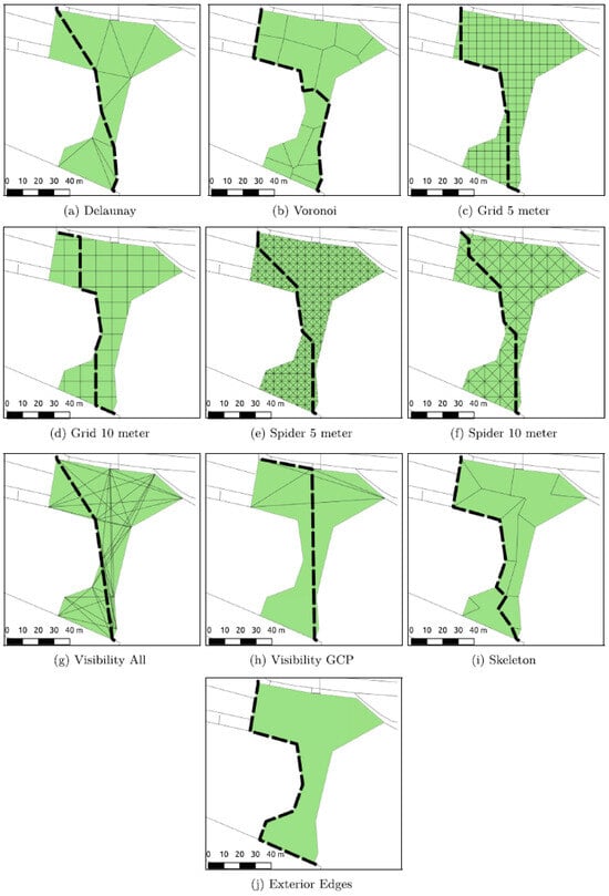
Figure 1.
Examples of different algorithms for producing a subgraph and the route suggested by each from the top left of the park to the bottom right: (a) Delaunay separates the space into triangles which are balanced in size and shape; (b) Voronoi tries to split the spaces into equal sized areas; (c,d) Grid divides the area into a grid at two different resolutions; (e,f) Spider adds additional complexity splitting the grids into triangles at the same resolutions; (g) Visibility divide the space by using lines of sight from entrances and exits of the park; (h) Visibility GCP is a modified version of (g) that removes connections that are not linked to the network; (i) Skeleton shrinks the edges of the area until they meet and then divides based on the meeting points; (j) Exterior Edges only uses the boundaries of the area to create the subgraph [8].
The ability to avoid obstacles, such as impassable terrain, rivers, or walls, is an important feature of routing algorithms in open areas. Graser [9] examined the directness and realism of routes incorporating obstacles, comparing Grid, Visibility, Medial Axis, and Straight Skeleton graphs (Figure 2), concluding that Visibility was the most suitable subgraph for open area routing. The Medial Axis and the Straight Skeleton routes create S-shaped routes, which were considered unnecessary detours and not characteristic of normal crossing behaviour (Figure 2A,B). Alternatively, the 5-m Grid gave a zigzag pattern (Figure 2C). This is a typical problem with grid-based solutions [8], where diagonal directions have poorer results compared to the north–south or east–west routes. It is worth noting that Graser [9] did not justify the orientation nor the resolution of the grid proposed. Both of these factors may significantly alter the quality of the routes. Visibility was found to provide the most preferable routes in terms of directness and realism (Figure 2D), although Graser [9] did not take advantage of the existing route network in the mapped area, only creating routes using the Visibility graph. However, this was only demonstrated on an open space polygon, which lacked obstacles. The treatment of obstacles in Visibility graphs depends on where the corner nodes of the obstacle are defined and increases in sophistication with more complex obstacles [10].
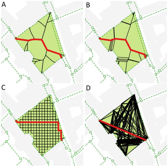
Figure 2.
Additional subgraph options on a different open area suggested by Graser [9]: (A): Medial Axis, built from a set of points that have more than one closest neighbour on the polygon boundary (often approximated by the Voronoi diagram); (B): Straight Skeleton, built by step-wise shrinking of the polygon; (C): 5 m Grid, which is a simple square grid with a cell size of 5 m; (D): Visibility, where nodes that have visible (straight-line) connections are linked.
Open areas typically contain a mixture of mapped path networks and freely traversable terrain. Andreev [5] implemented Visibility graph algorithms in parks and plazas while integrating sidewalks and walkways (paths). In plazas, the Visibility graph is a structure similar to that of Graser [9]. Obstacles were also accounted for in a similar way. Paths that are integrated into parks were preferred compared to ‘virtual’ paths due to being actual walkable areas. In addition, the ability to start the walk at any point in the park was achieved by creating a new Visibility graph from the point to the closest path or walkway. One shortcoming is that Andreev [5] evaluates the algorithm based on two examples, which does not capture the complexity of open space navigation.
2.2. Multi-Criteria Routing
In problems that involve routing on transportation networks, it is often desirable to choose routes according to multiple criteria, such as distance, travel time, and comfort, and Multi-Criteria Decision-Making (MCDM) has become increasingly popular in this domain [6,11,12]. Multi-criteria are combined to generate weightings, which are then fed into a standard shortest path algorithm, such as Dijkstra’s algorithm or A* [6].
The most popular MCDM method is the Weighted Sum method (WSM) (Equation (2)) and is demonstrated in [6]. This involves normalisation of all the criteria by dividing each value by the total of the criteria (Equation (1)). This weighted sum value then becomes the cost for each edge in the calculation of the shortest path. The benefit of WSM is that the results are easily explainable.
where = the normalised criterion value, = criterion value.
where = WSM Value, = the normalised criterion value, w = weight for criterion.
Alternatively, Rosita et al. [13] suggested using the vector normalisation technique to normalise values before applying a WSM. This allows a cost (Equation (3)) or a benefit (Equation (4)) criterion to be implemented into Dijkstra’s algorithm. These normalised values are then converted to a WSM value in the same way as in [6] (Equation (2)). The justification for the vector-normalised approach is that it allows easier integration of criteria into Dijkstra’s algorithm by inputting a value that could be a cost or a benefit to the same dimension. However, once normalised, the values can be very difficult to interpret without additional context.
where = the normalised criterion value, = criterion value.
Ebrahimi and Tadic [11] used MCDM to produce route selection when transporting dangerous goods. The seven criteria used to evaluate the routes, such as cost of transport or environment and accident risk, were given significance scores between 1 and 10, with 10 being most important. These values were decided by experts and then converted to weights using additive normalisation, which involves dividing the values by the sum of all significance values [11]. The criteria for each road link are normalised using percentage normalisation and then converted to a WSM value similar to [6]. One of the shortcomings of this method is there is no justification for the significance of each of the criteria beyond them being an ‘expert opinion’.
Pamucar et al. [12] demonstrated an alternative approach using Weighted Linear Combination (WLC) of raster datasets, a tool commonly used in GIS [14]. In this method, the raster cells are transformed (normalised) so that the units are standardised between the datasets. After normalisation, each raster cell is multiplied by its assigned criteria weight, and then each raster layer has its corresponding cell added to WSM (Figure 3). The bi-linear interpolation is then used to convert the average of the cell to the line (road) segment [12]. Pamucar et al. [12] used 21 different criteria to propose routes for more and less environmentally friendly vehicles to improve air quality in populated areas. The shortcoming of this technique is that it expects the input data as a raster, and requires a large amount of preprocessing before the weightings can be defined, which scales poorly with the number of criteria.
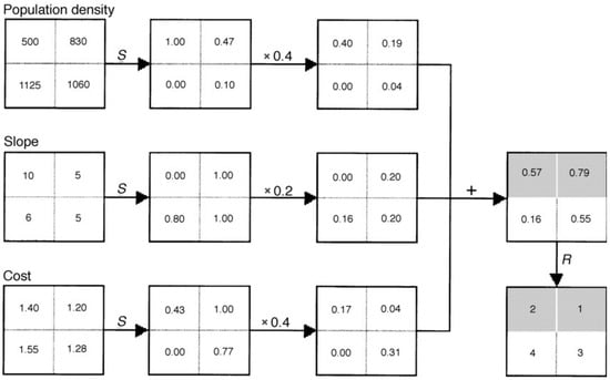
Figure 3.
Steps involved in a Weighted Linear Combination process. Given three raster layers—Population density, Slope, and Cost—the raw values are first normalised (in this case, using inverse MinMax normalisation where minimum values of each layer become 1, and maximum values become 0). Then, values in each layer are multiplied by each layer’s normalised criteria weight, after which each criteria value is added for each cell to produce final raster values.
In the domain of routing across open spaces, MCDM has found application in the planning and design of forest road routes. Caliskan [7] used the Spatial-integrated Technique for Order Preference by Similarity to Ideal Solution (S-TOPSIS) approach to integrate data on avalanche, river, soil, geology, and slope for forest road routing. A detailed study on TOPSIS can be found in [15]. When compared with the existing forest road, the S-TOPSIS solution gave a shorter route, translating to a 0.5 ha reduction in required road space. Caliskan [4] carried out a similar study in the Trabzon Province of Turkey, comparing five MCDM methods: Analytical Hierarchical Process (AHP), TOPSIS, Promothee, Fuzzy overlay, and SAW. The former three methods were found to perform best and produced very similar results. Of these, AHP and Promothee allow the user to decide pairwise relative importance of weights. This is a powerful approach in forest road routing, which is guided by expert stakeholders. However, it may not be suitable in general routing where the preferences vary between individuals.
2.3. Gaps in Relevant Work
A big difference between open areas in cities and open access land is that open access land can be entered from many points on its edge. In city parks and plazas, often a single-digit number of nodes is sufficient to represent points of access, whereas a walk in a national park can often start and end in any settlement or car park. This poses a challenge for a Visibility subgraph, which has to deal with a large number of edge nodes.
There is little academic literature on incorporating multi-criteria routing into human navigation. This is particularly important when considering that each user has different requirements and preferences due to their walking ability, reasons for walking, or safety requirements.
While commercial applications such as Strava, Komoot, and OS Maps App offer route planning services—allowing the routes to be modified based on popularity, terrain, and elevation, as well as manual routing options that allow route plotting when there are no paths—these solutions rely on ‘black box’ algorithms with unclear methodology. As such, it cannot be guaranteed the routes produced are conducive to walking. However, using the methods described by Pamucar et al. [12] and Ebrahimi and Tadic [11], a model traditionally used for motorised transport can be modified to work with a subgraph network, adapting a multi-criteria approach to pedestrian navigation in open spaces.
The choice of MCDM method changes how the weighting is defined, which can have a huge impact on the result [16]. Most of the research reviewed here uses subjective weightings defined by experts [11]. However, more understandable subjective weightings that have high explanatory power are available, such as ranking methods.
In summary, both routing over open areas and creating routes based on multiple criteria have been studied previously. However, to date, they have not been successfully applied to routing for access land. Additionally, pedestrian navigation in open areas in cities has key differences from navigation on access land, including the complexity of obstacles and hazards. In the following section, we will outline the materials and methods used to achieve the objectives of this research.
3. Materials and Methods
3.1. Materials
This subsection describes the datasets used to generate a routing network on access land, focusing on Dartmoor National Park, United Kingdom.
3.1.1. British National Grid
Extracted from the Ordnance Survey (OS) GitHub repository [17], this dataset contains grids at scales of 100 km, 50 km, 20 km, 10 km, 5 km, and 1 km in the OS National Grid reference system, commonly referred to as the British National Grid (BNG). The 1 km grid is used to define the spatial extent of the case study areas presented here.
3.1.2. Detailed Path Network
The Detailed Path Network (DPN) dataset contains a digital representation of all the roads, tracks, and paths in Dartmoor National Park that the public can use. It contains the geometry and physical characteristics of routes obtained from the OS MasterMap Topography Layer and the OS MasterMap Highways Network [18]. This dataset allows the incorporation of official paths including footpaths, bridleways, byways, and recreational routes into the subgraph network, which can then be used to give routing suggestions based on walking on reliable existing paths or with a mixture of ‘virtual’ paths based on the user preference.
3.1.3. MasterMap Topography
MasterMap topography dataset represents the real-world topography using points, lines, and polygons [19,20]. Features contain attributes that inform users about their presence and location in BNG coordinates. MasterMap topography includes buildings, land, water, and roads. This study focuses on land and water features. Land features include man-made and natural features such as slopes and cliffs. Water features include rivers and lakes [19]. The relevant attributes include descriptive group, descriptive term, and physical presence, which are used in intelligent querying and identification of obstructions and hazards.
3.1.4. Terrain 5
Terrain 5 is a digital terrain model (DTM), which is a three-dimensional model of the surface of the bare earth [21]. The dataset is interpolated from the OS Triangulated Irregular Network (TIN) [21]. This is a digital three-dimensional model of the surface morphology of Great Britain segmented using triangles. Mean high- and low-water representations have been acquired from local tide tables. Each height has a root mean square error (RMSE) of 2.5 m in mountain, rural, and moorland areas. In this study, the height values for each node are extracted from the pixel.
3.1.5. Devon County Council Access Land and Dartmoor Commons
Access Land and Dartmoor Commons is a dataset that includes polygons that define areas mapped as access land [22]. Areas of land designated as access land in the UK are defined as those that the public can walk across without having to stay on public rights of way. On Dartmoor, these are areas created by the Countryside and Rights of Way (CROW) Act 2000, such as Registered Commons and Open country, Registered Commons defined by the Dartmoor Commons Act of 1985, access land that was defined before the CROW Act 2000 covered in section 15, such as National Trust Common Act and Law of property Act of 1925, and finally section 16 of the CROW Act 2000, which includes lands voluntarily made access land by land owners, which are not moorland or registered common land [23].
3.1.6. Dartmoor National Parks Authority Habitat Classification Map
The Habitat Classification map is a land cover raster map of Dartmoor National Park represented as a m grid classification of habitats, which was created using Sentinel-2 and Lidar data [24]. The chosen characteristics were Sentinel-2 bands, vegetation indices, aspect, and slope (extracted from Lidar data) [24]. Classification was performed using a trained random forest classifier, and the 2021 land cover map achieved an accuracy of 76.9% [24]. The classified habitats were taken from the UK Habitat Classification System (Table 1).

Table 1.
Class labels and accuracy used for land cover compared to the land cover classification from the UK Centre for Ecology and Hydrology Land Cover Map (CEH LCM2019), modified from [24].
This dataset is important to incorporate as it informs us of the vegetation that is present on Dartmoor. This can then be converted into the cost of walking over different types of habitat classes, where areas with easy terrain are assigned a low cost and vice versa.
3.1.7. OS Maps User Generated Routes
This dataset contains user routes extracted from the OS Maps app, spanning the period from April 2019 to May 2022. To ensure data quality, a two-step filtering process was applied. First, duplicate routes based on geometry were removed. Second, routes exceeding a distance threshold of 10 m between consecutive GPS points were excluded. This threshold aimed to eliminate manually created routes or those recorded while the user was inside a vehicle. The total number of user routes extracted was 1353. By implementing these filters, we ensure the dataset comprises walking routes collected during actual navigation, and can be used to assess the quality of routes generated by the routing algorithms.
3.2. Methods
3.2.1. Creating a Spider-Grid Subgraph
To enable users to route from one node to another and to cope with the complexities of obstructions and hazards, a Spider-Grid was chosen instead of the popular Visibility diagram as the subgraph. A 25-m Grid was chosen to balance the computational time with the level of detail to enable accurate routing based on the selected criteria.
The following subsections describe a step-by-step process of creating the subgraph. The process is illustrated in Figure A1 in the Appendix A.
Node Creation
The 1 km bounding dimensions for the grid are extracted from the OS British National Grid dataset. A grid is generated with nodes placed at 25-m spacing along the X and Y axes (Figure 4A). Using the Terrain 5 DTM, the elevation is then extracted for each point.
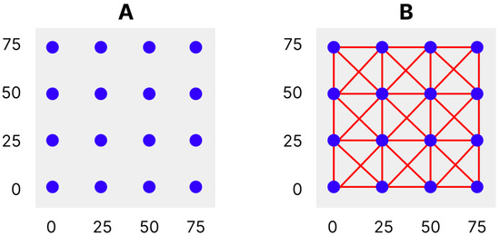
Figure 4.
(A): An illustration of nodes created for a subgraph at 25 m resolution in both x and y axes. (B): The same subgraph, but with queen contiguity links.
Link Creation
To create links between the nodes, queen contiguity is used. In queen contiguity, the primary cell is linked to all eight adjacent grid cells (see Figure 4B).
From the newly created links, the length is extracted using BNG. The elevation for each node is extracted from the Terrain 5 dataset, and is used to calculate the height change for each link. Height changes are subsequently used to calculate the gradient and the time to cross each link in minutes. The angle of gradient for each link is calculated using simple trigonometry with the length of the link and the change in height. Naismith’s rule, which considers distance and elevation gain, is used to estimate the average total time to cross each link in minutes [25]. The rule assumes a 5 km/h walking speed. The link length is divided by 5 (km/h) and then by 60 (minutes/hour) to give the base travel time in minutes. To account for elevation gain, one minute is added per 10 m of ascent.
3.2.2. Enhancing the Subgraph
This subsection discusses incorporating datasets to enhance the subgraph by removing hazards and obstacles, integrating a path network, and defining a terrain coefficient.
Integrating a Path Network
The path network (PN) is integrated by extracting paths within the bounds of the subgraphs using an intersection query. To add the PN, each path is converted into segments of its coordinates. The intersection coordinates collected are used to find the corresponding links in the subgraph network to include the PN path (Figure 5A). Located subgraph links are split into two links: one from the start to the intersecting point and one from the intersecting point to the end of the link.
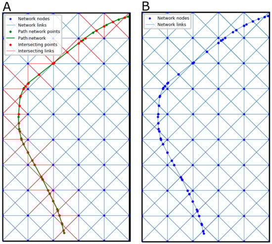
Figure 5.
(A): Example identification of intersecting points with subgraph. Points in red represent the intersecting points and lines in red represent the link they correspond with. (B): Fully integrated example of PN path into the subgraph.
The intersection points are added to the coordinates of the original PN path line string segments. The new line is broken into individual links using new coordinates. These links are given attributes such as length, gradient, and climbing time, using the method described in the Link creation subsection above. The converted PN links and points are combined into the network, leaving a new network with an integrated PN (Figure 5B). The advantage of this approach is that detailed information about existing paths is not lost in the subgraph.
To incorporate the PN into a shortest-path algorithm, a cost is needed. We use binary weighting; PN links receive a cost of 0, which means they are free of additional cost and are the preferred path, while other links receive a cost of 1.
Removing Obstructions, Hazards and Private Land
To prevent routes from being created in private or hazardous areas, links and nodes in these areas must be removed. A spatial intersection is used to remove nodes and links that intersect with areas defined as slopes, cliffs, rocky outcrops, and obstructions such as boundaries and watercourses (as illustrated in Figure 6). An exception is made if the PN is present, as these paths can be permissive footpaths offering safe navigation of hazards, such as a bridge intersecting a body of water, or a gate (stile) intersecting an obstruction such as a wall.
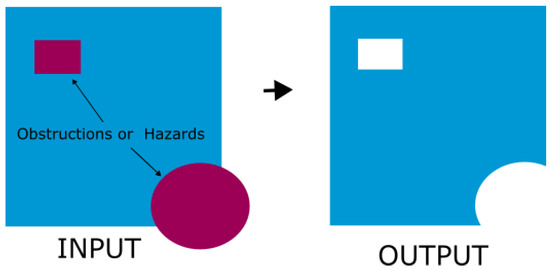
Figure 6.
Example of spatial intersection to only leave blue area (access land) with maroon objects signifying hazards, obstructions, or private land.
Incorporating Land Cover
The high resolution and variety of the Habitat Classification map allows the enhancement of the links by incorporating terrain conditions. Classification values are extracted from the raster for each node and link. A cost is applied to each habitat based on the effect that land cover has on walking.
Studies have shown that terrain affects walking speed, energy consumption, and mood. Taylor et al. [2] established that nine out of ten people agreed that the terrain they walked on affected their walking pace. Thus, an accurate value (terrain coefficient) is required to quantify the effect of terrain on walking speed [2,26]. This is particularly important for routing across open access land, where suggested routes do not have to stick to paths or roads and can incorporate a variety of different terrains.
In the literature, two approaches have been taken to measure a terrain coefficient: measuring oxygen consumption to calculate the energy cost [3,27,28] and comparing travel times over different terrains [29]. In our study, we use Herzog’s paper on terrain coefficients [30], which reviewed a number of coefficients from previous studies (see Table 2 and Equation (5)). Approximations were made for land covers not covered by these studies [24].
Table 2.
Terrain coefficients for different terrains as compiled by Herzog [30].
Energy cost prediction equation:
where M = metabolic rate (kcal/hr), = terrain factor defined as 1 for treadmill walking, W = body weight (kg), L = external load (kg), V = walking speed (km/hr), and G = slope (grade) expressed as percentage, as presented in [3].
The urban land cover classification refers to “constructed, industrial and other artificial habitats” [24]. In the subgraph, this refers to roads and man-made tracks primarily covered by rock or asphalt. According to Soule and Goldman [3], roads offer optimal surface conditions for walking due to their high level of visibility and smooth terrain with little difference compared to walking on a treadmill. These are assigned the terrain coefficient of 1.0 (Table 2 and Table 3). Acid grasslands and modified grasslands are associated with low-growing habitats such as fine grasses and low-growing herbs (Figure 7A) [31]. The closest association is grass, and therefore a terrain coefficient of 1.1 is used (Table 2 and Table 3).
Table 3.
Terrain coefficient scores assigned to each land cover classification.
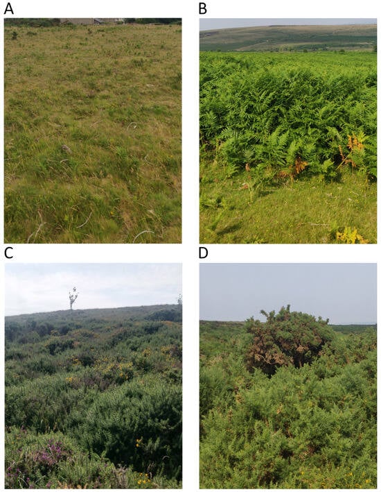
Figure 7.
Images of different land covers at Haytor Down. (A): Acid grassland; (B): Braken; (C): Heathland; (D): Gorse.
Bracken and meadow habitats are associated with ‘light brush’ and receive a terrain coefficient of 1.2. (Table 2 and Table 3). Cropland is generalised to the terrain coefficient of the ‘ploughed field’ of 1.3. Woodlands are associated with the terrain coefficient of the ‘heavy brush’, although different forests have varying impacts on walking [32] (Table 2 and Table 3). Heath land is also associated with the ‘heavy brush’ terrain coefficient (Figure 7C) [31].
Habitats near peat deposits and impoverished soils, such as blanket bog and purple moor grass, are associated with ‘swampy bog’ (Table 2 and Table 3). Blanket bogs are almost permanently waterlogged, making traversal difficult [31]. Acid grass and unvegetated degraded blanket bogs have some uncertainty in defining their terrain coefficient. Degraded blanket bogs are areas where drainage has caused the loss of peat-forming species that have been overlain with other vegetation [24]. Association with blanket bogs suggests a terrain coefficient close to ‘swampy bog’, but loss of peat-forming species suggests a lower coefficient. To account for this uncertainty, a terrain coefficient was defined in between (Table 2 and Table 3).
According to Herzog [30], some vegetation provides difficult or highly hazardous terrain and is given an extremely high terrain coefficient to demonstrate the likelihood of obstruction or hazard (Table 3). Gorse scrub land dominates this category on Dartmoor, and although its closest terrain coefficient is heavy brush, its height and high density make it extremely difficult to traverse (Figure 7D) [33].
3.2.3. Creating Routes
The next step is to create routes in the subgraph. We used Weighted Sum–Dijkstra’s algorithm to create routes based on multiple criteria.
Single Criterion vs. Multi-Criteria Routes
To create these routes, we follow a similar process to that of Kien Hua and Abdullah [6]. This involves using a Weighted Sum-Dijkstra’s algorithm, which combines WSM with Dijkstra’s algorithm. WSM requires that the criteria values for each link are normalised (Equation (1)). Each criterion is then multiplied by the weight of the criteria to produce the final value of the criteria. This value is then summed with the other criteria values to obtain a WSM value for each link (Equation (6)).
Weighted Sum method equation modified for specific criteria:
where = sum of all the final criteria values, = normalised gradient value for the link, = normalised weight for the gradient criterion, = normalised Path Network value for the link, = normalised weight for the Path Network criterion, = normalised terrain coefficient value for the link, = normalised weight for the terrain coefficient criterion, = normalised total time value for the link, and = normalised weight for the total time criterion.
Converting Criteria to Be Implemented in Dijkstra’s Algorithm
Due to the nature of Dijkstra’s algorithm, we need to adjust the gradient, terrain coefficient, and PN values to be proportional to the length of each link. This normalisation is achieved by multiplying each link’s criterion value by its length.
Choosing a Weighting Method
Choosing the correct weighting for the routes is important, as different weights will change the outcome of the routes. While previous studies have used sophisticated methods such as TOPSIS and AHP, these are more suited to problems where a single ideal solution is sought, such as forest road routing. In the case of walking routes, weightings are subject to change based on user preferences, so should be easy to adjust. Therefore, subjective weightings were chosen because they reduce computational complexity and are easy to explain and understand [16]. The ranking method was chosen to assign criteria weights due to their simplicity when the number of attributes is low [16]. Ranking methods include three ways to calculate weights: rank sum, rank exponent (see Equation (7)) and reciprocal rank. Each process requires ranking the attributes from most to least important. After calculating the weights, they are normalised by dividing each weight by the sum of all the weights.
Rank exponent:
where n = number of ranking attributes, r = rank given to the criteria, and p = exponential parameter chosen by the user.
We chose the ranking exponent method due to the flexibility of adjusting the exponential parameter p [34]. To determine the most suitable exponential parameter p, weights were calculated using a value of zero to five similar to [35]. Three was chosen as it provided a sufficiently steep weight distribution for the most important criteria to be the dominant route decider. This was particularly important for routes that needed to preferentially follow the PN, where if p was less than four, the routes significantly deviated from the PN, while a p of five produced the same result as a single criterion method.
For simplicity, walking ability was divided into three categories: easy, intermediate, and challenging, based on similar factors to route grading by OS Maps App, Ramblers England, and Komoot [36,37,38] (Table 4). Referring to the classification from the OS Maps App and Ramblers England, an easy walking ability (EWA) route should be generally flat, be completely on the PN, and be on a well-paved surface. Intermediate walking ability (IWA) is for the average walker with surface condition and gradient becoming a less important factor. However, this classification still primarily follows the PN for easier navigation. Challenging walking ability (CWA) is focused on including more flexibility on the suggested route, and criteria such as staying on footpaths and gradient of the route are less important.
Table 4.
Characteristics of route difficulty defined by Ordnance Survey Maps [36].
These preferences are then converted into rankings (Table 5), which in turn are converted to weightings using the ranking exponent and normalised (Table 6). An example of the impact of the weightings and rankings on the network can be seen in Figure 8.
Table 5.
Ranking assigned to each walking ability and criteria.
Table 6.
Rankings converted into normalised weightings for each walking ability using rank exponent.
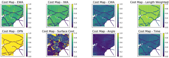
Figure 8.
Cost Maps for all the weightings in the Spider-Grid algorithm. © Crown copyright and/or database rights 2022 OS (Research Licence).
The routing algorithm is implemented in Python and uses the following packages: Shapely, NetworkX, Rasterio, and GeoPandas [39,40,41,42].
4. Evaluation Methods
4.1. Study Areas
Haytor Down (SX 7677) and Hound Tor (SX 7478)
Haytor is one of the most famous tors on Dartmoor (Figure 9). It draws tourists due to panoramic views of Dartmoor from the top of Haytor Rocks and its accessibility from major roads. The area contains a large number of footpaths, which can be used to test the integration of the PN. In addition, Haytor Down incorporates large areas of private land to the south-east, and a large number of obstructions such as streams and rocky slopes, which will help test the algorithm’s ability to distinguish and remove such features.
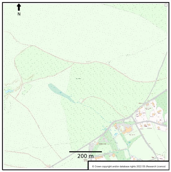
Figure 9.
Ordnance Survey MasterMap extract of Haytor Study area. © Crown copyright and/or database rights 2022 OS (Research Licence).
In contrast, Hound Tor offers a more complex test environment due to its abundance of walls and obstructions in the study area, limiting potential user paths. Furthermore, prominent rocky outcrops like Hound Tor and Greator Rocks require clear identification and removal as they pose safety hazards.
4.2. Routes
To compare the Weighted Spider-Grid with other network-based routing graphs, the start and end points of the user generated routes were extracted and used for routing. A Visibility graph network was created using the pyvisgraph [43] Python package, and combined with obstructions to create a direct comparison to the Weighted Spider-Grid. A non-weighted version of the Spider-Grid was also created to compare the effectiveness of weighting criteria.
Criteria chosen to evaluate the generated routes are as follows:
- Average PN as %: average percentage of the route that is on the Path Network;
- Average surface cost: average surface cost score over all the routes;
- Average gradient in degrees: average gradient change across all routes;
- Average total time in minutes: estimated average walking time in minutes across all routes, calculated using Naismith’s rule;
- Average total length in metres: average distance of the routes in metres.
Furthermore, to visually compare the generated routes with user routes, line density maps were created and overlaid to identify areas of common intersection. This analysis provides insights into the quality of the generated routes by assessing their alignment with real user preferences.
5. Results and Discussion
Table 7 and Table 8 show how different routing algorithms scored on average across five metrics. In the tables, Unweighted refers to Dijkstra’s algorithm without multi-criteria weights. EWA, IWA, and CWA use the different weighting schemes outlined in Table 6. Although several previous studies highlighted the efficacy of Visibility graphs for open areas [5,8,9], the results suggest it may not be the most suitable for complex open areas. Although the Visibility-generated routes offer slightly quicker and shorter routes, only about 10% of the Visibility routes follow the existing PN. This can be seen in Figure 10 and Figure 11, where the Visibility routes have very little overlap with the user-generated routes.
Table 7.
Comparative results for each routing algorithm for Haytor.
Table 8.
Comparative results for each routing algorithm for Hound Tor.
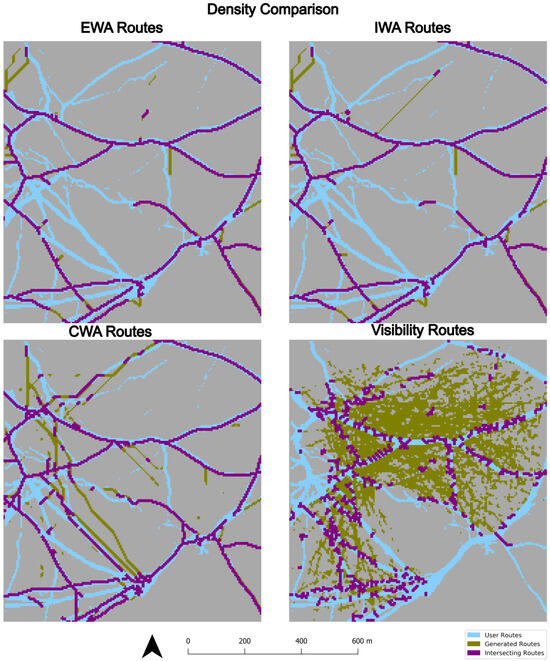
Figure 10.
Density Comparison of the routes generated and the user routes for Haytor. © Crown copyright and/or database rights 2022 OS (Research Licence).
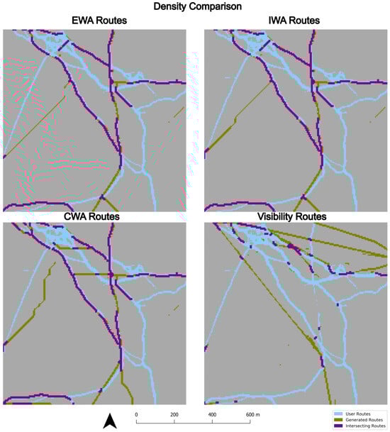
Figure 11.
Density Comparison of the routes generated and the user routes for Houndtor © Crown copyright and/or database rights 2022 OS (Research Licence).
In addition, Visibility routes have high surface costs, indicating the presence of harder-to-walk terrain such as heavy brush (Table 3). In comparison, the CWA routes have a surface cost that is closer to that of grass and dirt roads (Table 3), which is more conducive to walking, while only being 50 m longer on average for Haytor. This can be seen when comparing the density overlap of the CWA routes to the Visibility routes in Figure 10 and Figure 11, where the CWA routes have a much higher overlap than the Visibility routes.
One limitation of the current algorithm is a mismatch of obstructions between the real world and the MasterMap Topology dataset, as observed in the southeastern portion of Houndtor. During the creation of the Spider Grid, a large number of nodes and links were removed from this area due to the presence of numerous walls and other obstacles. Consequently, it was impossible to generate routes in this region for comparison with the user routes. This limitation appears to stem from the MasterMap Topography dataset, which seems to lack up-to-date information regarding where walls exist that users can traverse.
Interestingly, EWA and IWA routes have very similar characteristics in terms of gradient, surface cost, and PN. Both algorithms prioritise using the PN (i.e., both have a PN rank of 1), which cause the calculated routes to remain on the PN for almost 89% of the routes in Hound Tor and over 96% in Haytor. Additionally, the EWA and IWA routes have an average surface cost in the range between 1.0 and 1.1, which suggests that the routes are likely to be easier to traverse if accessibility is an issue (Table 7). This preference seems to match the user largely with routes with both EWA and IWA having a high degree of intersection.
A likely explanation for this similarity between EWA and IWA is the high weighting of the PN, which prevents the IWA routes from deviating to routes that have significantly different characteristics.
In summary, the EWA and IWA routes are very similar, on average, to the user routes and offer the best routes when using the PN, a less challenging terrain, and a flatter gradient. Alternatively, CWA routes, which prioritise total time and ranks the PN% third, are indeed more off the footpaths, and shorter in both time and distance. Interestingly, for Haytor, they also offer the most similar routes to the user routes—a likely explanation is that the algorithm picks up ‘unofficial’ footpaths which are more direct towards the end point.
All three methods built using the Weighted Sum–Dijkstra’s algorithm are likely to be considered more favourable for walking compared to the Visibility routes due to their higher percentage of on-the-path network, lower surface cost, and less extreme gradient. And most importantly, they do resemble the actual user-generated routes.
6. Conclusions and Recommendations
In this paper, we proposed an algorithm for routing on access land that incorporates multi-criteria decision-making. The proposed approach uses a spider grid subgraph and a Weighted Sum–Dijkstra’s algorithm, and is tested on case studies in Dartmoor National Park. The algorithm is able to generate routes that consider multiple criteria such as gradient, surface cost, path network, and total time, with different criteria weights resulting in different route preferences. The algorithm performed better than other network-based routing methods such as Visibility graphs in terms of realism and flexibility of the routes. In particular, incorporating the existing PN and adjusting its weight provides routes tailored to a range of capabilities, from easy to challenging. These findings have implications for improving accessibility and safety of access land for walkers with different abilities and preferences. They also contribute to the existing literature on open area routing and multi-criteria decision making.
Moreover, this research has potential applications for other domains and scenarios related to access land. The results could be used to:
- Inform national park agencies on where to create alternative routes when erosion of the footpath means that a path must be diverted;
- Make protected habitats inaccessible to users and prevent further damage and disruption of local ecosystems;
- Provide alternative routing in emergency scenarios, such as finding the most favourable route for the evacuation of people due to flooding or landslides.
Some directions for future research include testing the algorithm on other areas of access land with different characteristics and data sources, incorporating user feedback and preferences into the route generation process, and developing a user-friendly interface for the algorithm.
Author Contributions
Conceptualization, Rafael Felipe Sprent and Stefano Cavazzi; Methodology, Rafael Felipe Sprent and James Haworth; Software, Rafael Felipe Sprent and Stefano Cavazzi; Supervision, James Haworth; Writing—original draft, Rafael Felipe Sprent; Writing—review & editing, Rafael Felipe Sprent, James Haworth, Ilya Ilyankou and Stefano Cavazzi. All authors have read and agreed to the published version of the manuscript.
Funding
This research received no external funding.
Institutional Review Board Statement
Not applicable.
Data Availability Statement
Data available in a publicly accessible repository: Gatis, N.; Carless, D.; Luscombe, D.J.; Brazier, R.E.; Anderson, K., 2022, Dartmoor National Parks Authority Habitat Classification Map, https://ore.exeter.ac.uk/repository/handle/10871/129968 (accessed on 1 August 2022) Data available in a publicly accessible repository that does not issue DOIs: Ware, G., 2017, Access Land & Dartmoor Commons, https://data-dcc.opendata.arcgis.com/datasets/access-land-dartmoor-commons (accessed on 2 August 2022) Ordnance Survey, 2021, OS British National Grids, https://github.com/OrdnanceSurvey/OS-British-National-Grids (accessed on 2 August 2022) Data available on request (licensing restrictions apply): Ordnance Survey, 2022, OS Terrain 5, https://www.ordnancesurvey.co.uk/products/os-terrain-5 (accessed on 2 August 2022) Ordnance Survey, 2022, OS Detailed Path Network, https://www.ordnancesurvey.co.uk/business-government/products/path-network (accessed on 2 August 2022) Ordnance Survey, 2022, MasterMap Topography Layer, https://www.ordnancesurvey.co.uk/business-government/products/mastermap-topography (accessed on 2 August 2022) Ordnance Survey, 2022, User Generated Routes.
Conflicts of Interest
Author Stefano Cavazzi is employed by the Ordnance Survey. The authors declare no conflict of interest.
Abbreviations
The following abbreviations are used in this manuscript:
| PN | Path Network |
| OS | Ordnance Survey |
| EWA | Easy Walking Ability |
| IWA | Intermediate Walking Ability |
| CWA | Challenging Walking Ability |
| MCDM | Multi-Criteria Decision Making |
| WSM | Weighted Sum Method |
Appendix A


Figure A1.
Complete subgraph creation process for Haytor Down. (A): Node creation, (B): Link creation, (C): Detailed Path Network integration, (D): Non access land removal, (E): MasterMap polygon layer removal, (F): MasterMap line layer removal. © Crown copyright and/or database rights 2022 OS (Research Licence).


References
- Ramblers. Access to Open Countryside—Ramblers, 2020. Available online: https://www.ramblers.org.uk/policy/england/access/access-to-wild-open-countryside-or-the-right-to-roam.aspx (accessed on 24 August 2022).
- Taylor, K.L.; Fitzsimons, C.; Mutrie, N. Objective and subjective assessments of normal walking pace, in comparison with that recommended for moderate intensity physical activity. Int. J. Exerc. Sci. 2010, 3, 87. [Google Scholar]
- Soule, R.G.; Goldman, R.F. Terrain coefficients for energy cost prediction. J. Appl. Physiol. 1972, 32, 706–708. [Google Scholar] [CrossRef]
- Çalişkan, E.; Bediroglu, Ş.; Yildirim, V. Determination forest road routes via GIS-based spatial multi-criterion decision methods. Appl. Ecol. Environ. Res. 2019, 17, 759–779. [Google Scholar] [CrossRef]
- Andreev, S.; Dibbelt, J.; Nöllenburg, M.; Pajor, T.; Wagner, D. Towards Realistic Pedestrian Route Planning. In Proceedings of the 15th Workshop on Algorithmic Approaches for Transportation Modelling, Optimization, and Systems (ATMOS 2015), Patras, Greece, 17 September 2015; Italiano, G.F., Schmidt, M., Eds.; Schloss Dagstuhl–Leibniz-Zentrum fuer Informatik: Dagstuhl, Germany, 2015; Volume 48, pp. 1–15, ISSN 2190-6807. [Google Scholar] [CrossRef]
- Kien Hua, T.; Abdullah, N. Weighted Sum-Dijkstra’s Algorithm in Best Path Identification based on Multiple Criteria. J. Comput. Sci. Comput. Math. 2018, 8, 107–113. [Google Scholar] [CrossRef]
- Çalişkan, E. Planning of environmentally sound forest road route using GIS & S-MCDM. Šumarski List 2017, 141, 583–591. [Google Scholar] [CrossRef][Green Version]
- Hahmann, S.; Miksch, J.; Resch, B.; Lauer, J.; Zipf, A. Routing through open spaces—A performance comparison of algorithms. Geo-Spat. Inf. Sci. 2018, 21, 247–256. [Google Scholar] [CrossRef]
- Graser, A. Integrating Open Spaces into OpenStreetMap Routing Graphs for Realistic Crossing Behaviour in Pedestrian Navigation. GI_Forum 2016, 1, 217–230. [Google Scholar] [CrossRef][Green Version]
- Chen, Y.; Wu, G.; Zhao, T.; Chen, F. An Approach for Generating Pedestrian Network Based on Improved Navigation Graph. Int. J. Hybrid Inf. Technol. 2017, 10, 21–32. [Google Scholar] [CrossRef]
- Ebrahimi, H.; Tadic, M. Optimization of dangerous goods transport in urban zone. Decis. Mak. Appl. Manag. Eng. 2018, 1, 131–152. [Google Scholar] [CrossRef]
- Pamučar, D.; Gigović, L.; Ćirović, G.; Regodić, M. Transport spatial model for the definition of green routes for city logistics centers. Environ. Impact Assess. Rev. 2016, 56, 72–87. [Google Scholar] [CrossRef]
- Rosita, Y.D.; Rosyida, E.E.; Rudiyanto, M.A. Implementation of Dijkstra Algorithm and Multi-Criteria Decision-Making for Optimal Route Distribution. Procedia Comput. Sci. 2019, 161, 378–385. [Google Scholar] [CrossRef]
- Malczewski, J. On the Use of Weighted Linear Combination Method in GIS: Common and Best Practice Approaches. Trans. GIS 2000, 4, 5–22. [Google Scholar] [CrossRef]
- Lakshmi, M.T.M.; Vetriselvi, K.; Anand, A.J.; Venkatesan, D.V.P. A Study on Different Types of Normalization Methods in Adaptive Technique for Order Preference by Similarity to Ideal Solution (TOPSIS). Int. J. Eng. Res. 2016, 4. Available online: https://www.ijert.org/research/a-study-on-different-types-of-normalization-methods-in-adaptive-technique-for-order-preference-by-similarity-to-ideal-solution-topsis-IJERTCONV4IS05004.pdf (accessed on 21 March 2024).
- Odu, G.O. Weighting methods for multi-criteria decision making technique. J. Appl. Sci. Environ. Manag. 2019, 23, 1449–1457. [Google Scholar] [CrossRef]
- Glynn, C. OrdnanceSurvey/OS-British-National-Grids: A Free Set of Grids at Various Resolutions for Ordnance Survey’s National Grid. 2021. Available online: https://github.com/OrdnanceSurvey/OS-British-National-Grids (accessed on 2 August 2022).
- Ordnance Survey. Os-Detailed-Path-Network-Product-Guide, 2017. Available online: https://www.ordnancesurvey.co.uk/products/os-detailed-path-network (accessed on 2 August 2022).
- Ordnance Survey. Os-Mastermap-Topography-Layer-Technical-Specification, 2017. Available online: https://www.ordnancesurvey.co.uk/products/os-mastermap-topography-layer (accessed on 2 August 2022).
- Ordnance Survey (GB). OS MasterMap ® Topography Layer [GeoPackage Geospatial Data], 2021. Available online: https://digimap.edina.ac.uk (accessed on 2 August 2022).
- Ordnance Survey. Os-Terrain-5-User-Guide, 2017. Available online: https://www.ordnancesurvey.co.uk/products/os-terrain-5 (accessed on 2 August 2022).
- Ware, G. Access Land & Dartmoor Commons, 2017. Available online: https://data-dcc.opendata.arcgis.com/datasets/access-land-dartmoor-commons (accessed on 30 September 2022).
- Ramblers. Access Land in England and Wales—Ramblers, 2022. Available online: https://www.ramblers.org.uk/accessguide (accessed on 24 September 2022).
- Gatis, N.; Carless, D.; Luscombe, D.J.; Brazier, R.E.; Anderson, K. An operational land cover and land cover change toolbox: Processing open-source data with open-source software. Ecol. Solut. Evid. 2022, 3, e12162. [Google Scholar] [CrossRef]
- Naismith, W.W. Cruach Ardran, Stobinian, and Ben More. Scott. Mt. Club 1892, 2, 135. [Google Scholar]
- Gast, K.; Kram, R.; Riemer, R. Preferred walking speed on rough terrain; is it all about energetics? J. Exp. Biol. 2019, 222, jeb.185447. [Google Scholar] [CrossRef] [PubMed]
- Givoni, B.; Goldman, R.F. Predicting metabolic energy cost. J. Appl. Physiol. 1971, 30, 429–433. [Google Scholar] [CrossRef] [PubMed]
- Pandolf, K.B.; Givoni, B.; Goldman, R.F. Predicting energy expenditure with loads while standing or walking very slowly. J. Appl. Physiol. 1977, 43, 577–581. [Google Scholar] [CrossRef]
- de Gruchy, M.; Caswell, E.; Edwards, J. Velocity-Based Terrain Coefficients for Time-Based Models of Human Movement. Internet Archaeol. 2017, 45. [Google Scholar] [CrossRef]
- Herzog, I. Least-Cost Paths—Some Methodological Issues, 2014. Available online: https://intarch.ac.uk/journal/issue36/5/5-3.html (accessed on 5 September 2022).
- Butcher, B. UK Habitat Classification—Habitat Definitions, 2018. Available online: https://ecountability.co.uk/wp-content/uploads/2018/05/UK-Habitat-Classification-Habitat-Definitions-V1.0-May-2018-1.pdf (accessed on 1 August 2022).
- European Commission. Forest Observations, 2015. Available online: https://forobs.jrc.ec.europa.eu/products/gam/sources.php (accessed on 5 October 2022).
- John, T. Gorse, 2016. Available online: https://dartmoorlinks.co.uk/api/content/916d1ba6-54d5-11e6-ae0d-12955eaaf839/ (accessed on 31 August 2022).
- Gourisetti, S.N.G.; Mylrea, M.; Patangia, H. Application of Rank-Weight Methods to Blockchain Cybersecurity Vulnerability Assessment Framework. In Proceedings of the 2019 IEEE 9th Annual Computing and Communication Workshop and Conference (CCWC), Las Vegas, NV, USA, 7–9 January 2019; pp. 0206–0213. [Google Scholar] [CrossRef]
- Roszkowska, E. Rank Ordering Criteria Weighting Methods—A Comparative Overview. Optimum. Econ. Stud. 2013, 5, 14–33. [Google Scholar] [CrossRef]
- Ordnance Survey. Technical Difficulties, 2022. Available online: https://osmaps.com/technical-difficulties (accessed on 3 August 2022).
- Renzel, P. Ramblers Cymru—Key facts Report, 2018. Available online: https://www.ramblers.org.uk/-/media/Files/Wales%20microsite/Ramblers%20Cymru%20-%20Key%20Facts%20Report%202018.ashx (accessed on 1 August 2022).
- Komoot. Off-Grid Tour Planning Outside of Komoot’s Routing Network, 2022. Available online: https://support.komoot.com/hc/en-us/articles/360024733651-Off-grid-Tour-planning-outside-of-komoot-s-routing-network (accessed on 2 August 2022).
- den Bossche, J.V.; Fleischmann, M.; Jordahl, K. Geopandas/Geopandas: Python Tools for Geographic Data, 2022. Available online: https://github.com/geopandas/geopandas (accessed on 16 March 2024).
- Shavit, A.; Snow, A.D.; Rubiales, A.; Adair, A. Shapely—Shapely 2.0.3 Documentation, 2024. Available online: https://shapely.readthedocs.io/en/stable/index.html (accessed on 16 March 2024).
- Gillies, S. Introduction—Rasterio Documentation, 2021. Available online: https://rasterio.readthedocs.io/en/stable/intro.html (accessed on 16 March 2024).
- Hagberg, A.; Schult, D.; Swart, P. NetworkX—NetworkX Documentation, 2023. Available online: https://networkx.org/ (accessed on 16 March 2024).
- Reksten-Monsen, C.A. TaipanRex/Pyvisgraph: Given a List of Simple Obstacle Polygons, Build the Visibility Graph and Find the Shortest Path between Two Points, 2016. Available online: https://github.com/TaipanRex/pyvisgraph (accessed on 16 March 2024).


Disclaimer/Publisher’s Note: The statements, opinions and data contained in all publications are solely those of the individual author(s) and contributor(s) and not of MDPI and/or the editor(s). MDPI and/or the editor(s) disclaim responsibility for any injury to people or property resulting from any ideas, methods, instructions or products referred to in the content. |
© 2024 by the authors. Licensee MDPI, Basel, Switzerland. This article is an open access article distributed under the terms and conditions of the Creative Commons Attribution (CC BY) license (https://creativecommons.org/licenses/by/4.0/).