1. Introduction
Geocoding involves resolving the location information described in natural language text to the corresponding points or regions on Earth [
1,
2]. With the popularization of the Internet and social media, there has been a dramatic surge in textual data associated with geographic information [
3]. However, owing to privacy concerns, the availability of explicit geographic information, such as coordinates, on social media has gradually decreased. For example, Twitter discontinued explicit geographic information in 2019 and shifted to supporting implicit geographic information, such as POIs [
4]. Therefore, geocoding has become an indispensable tool for mining big data on location-related social media and effectively extracting geographic information. It plays an important role in urban planning, disaster emergency response, the geospatial analysis of social media, and disease risk mapping [
2,
5,
6].
Geocoding aims to parse unstructured text into structured spatial data, and its main output forms include geospatial coordinates, polygons, and entries into a geospatial database [
1,
2]. Previous geocoding systems relied mainly on external geospatial databases to match and sort text to be parsed with specific entries into the database [
7,
8,
9,
10,
11]. However, owing to its high reliance on external knowledge bases, this form of geocoding faces numerous obstacles in regions that lack standard geographic datasets or a GIS data infrastructure. In recent years, the application of end-to-end deep-learning models in geocoding tasks has gradually increased. This approach deepens the semantic understanding of address text and can directly predict geographical spatial labels from text with a straightforward workflow and low dependency on external databases such as gazetteers. It typically includes two primary methods: modeling as a regression task based on coordinate points or as a classification task based on regions such as grids or polygons [
1,
2,
3,
12,
13,
14,
15]. Due to the challenges involved in directly learning the mapping between text and precise coordinates in coordinate-point-based tasks [
15], some researchers prefer to model geocoding as a classification problem for predicting regions based on grids or polygons. Compared with approaches that use complex polygon structures for cities, states, and countries, geographic grids offer multi-level spatial representations without the need for external metadata, making them straightforward to understand and use. Therefore, this study focuses on grid-based classification methods for geocoding. This approach usually discretizes Earth’s surface into a series of grids and predicts the grid category corresponding to the input text based on a classification model to indirectly obtain geographical coordinates [
1,
2,
6,
13,
14,
15,
16,
17,
18]. Additionally, discrete global grid systems such as Geohash, H3, and S2 geometry play a crucial role in the spatial indexing, association, and geolocation of satellite and street-view imagery data [
16,
19,
20,
21,
22,
23,
24]. Recently, research on the spatial alignment of multimodal data, such as text and images, has increased [
25,
26,
27]. Parsing text into the corresponding geographic grids can provide a unified spatial foundation for these studies, offering extensive application prospects.
However, in fine-grained geocoding tasks with more detailed grid partitioning, the number of grid categories increases sharply. Taking the S2 grid as an example, when the average unit grid area is approximately 300 m², the global number of grids can reach 1649 billion. This leads to a serious dimensionality explosion in the output space, making it difficult for classification models to train and thus leading to a decrease in geocoding accuracy [
15,
28]. Moreover, most approaches generally overlook the inherent hierarchical structure characteristics of geographical grids and address text as well as the potential associations between them [
29,
30]. Unlike general texts, address texts often start with large-scale elements (e.g., countries and provinces) and are gradually refined into small-scale elements (e.g., specific buildings). Similarly, discrete global grid systems often recursively subdivide Earth from larger-scale grids into finer-scale grids. This structure implies that each sub-element (subgrid) represents varying hierarchies of geospatial information within a certain region and that text elements at different hierarchical levels often correspond to geographic grids of varying scales. Ignoring this feature may lead to the confusion of semantically similar but geographically different information [
30].
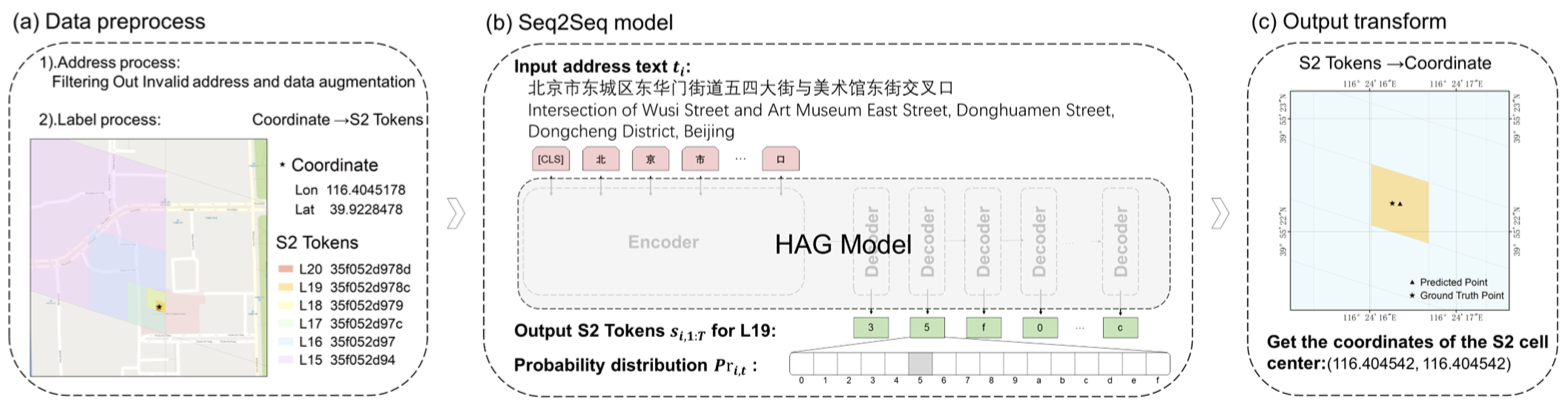
To address these challenges, we propose a novel hierarchy-aware geocoding model based on cross attention (HAGM), which is a grid-based geocoding method within a sequence-to-sequence (Seq2Seq) framework. This study utilized S2 geometry (
https://s2geometry.io/, accessed on 29 January 2024.) (a method for the hierarchical discretization of Earth’s surface) to map continuous latitude and longitude coordinates onto discrete geographic grids (S2 cells) to represent geographic locations. Compared with traditional classification models, HAGM within the Seq2Seq framework treats each character of the grid labels as an independent unit to be predicted and sequentially outputs them character by character; thus, it effectively avoids the issue of dimensionality explosion in the output space. Moreover, the HAGM employs a cross-attention module and a residual connection module to effectively and comprehensively perceive the hierarchical structure of address texts and geographic grids, and establish a correspondence between input address text elements at different hierarchical levels and geographic grids of varying scales.
Our main contributions are the following:
(1) Our proposed method effectively avoids the influence of output space dimensionality explosion and performs well in fine-grained geocoding tasks.
(2) The HAGM dynamically focuses on the contextual information of varying geographic scales, thereby enhancing its perception of the hierarchical characteristics and potential semantic associations of address text and S2 tokens.
(3) We evaluate the impact of different grid division scales on the performance of the geocoding model and compare it with previous methods in terms of multiple evaluation metrics in order to provide a thorough analysis.
(4) The performance of HAGM in the sparse data distribution region is significantly improved compared with the traditional classification model; this indicates that HAGM can mitigate the effects of imbalanced data distribution and overcome the problem of insufficient model learning in areas of sparse data distribution to some extent.
2. Related Work
Early geocoding research primarily employed rule-based and traditional machine learning methods combined with heuristic strategies to establish direct mapping relationships between text and locations, obtaining candidate entries from address databases and then ranking and selecting them [
7,
9,
31,
32,
33]. Although these methods have achieved satisfactory results, their frameworks are essentially based on indirectly predicting the corresponding geographic coordinates by ranking the similarities between the locations mentioned in the text and entries in a database, such as gazetteers. Owing to its high dependency on external databases, geocoding faces numerous obstacles in regions lacking standard geographic datasets or GIS infrastructure, leading to insufficient generalization capabilities [
5,
18,
29]. Therefore, researchers have begun to apply end-to-end deep learning models to geocoding in order to directly predict associated geographic spatial labels based on input query texts. This is often modeled as a coordinate point-based regression task and a grid-based or region-based multi-classification task [
12,
13,
15], with low dependence on external databases, such as gazetteers, and stronger generalization ability. Therefore, it is widely used in tasks such as event geocoding and Internet text geocoding [
34,
35].
In cases modeled as a coordinate-point-based regression task, researchers typically predict associated geographical coordinates directly from the input address text [
34,
35,
36,
37,
38]. For example, Liu et al. [
35] explored a method to estimate Twitter user locations using the textual data they generate on social media by utilizing a deep learning architecture constructed from stacked denoising autoencoders to directly predict the locations of users in terms of longitude and latitude. The results were comparable to those of the most advanced models at the time, demonstrating that this architecture is well-suited for geocoding tasks. Radford et al. [
34] proposed an end-to-end probabilistic model for geocoding the text of event data, directly predicting the latitude and longitude of the locations mentioned or described in a natural language. They also compared their model-based solution with previous state-of-the-art open-source geocoding systems and extensively discussed the benefits of end-to-end geocoding based on their models. However, these methods are insufficient for extracting the semantic features of a text. Hence, Xu et al. [
37] proposed a geo-semantic address model (GSAM) that supports various downstream tasks to deepen text features. Building on this, they incorporated three fully connected layers as hidden layers for the address location prediction task and added a final linear layer with two neurons to directly predict the coordinates (latitude and longitude). However, this regression-based approach to directly predicting geographic coordinates can cause issues with the continuity and infinity of the output space, resulting in learning difficulties for the model and often leading to serious degradation of the model performance owing to data quality issues.
Consequently, researchers tend to model the geocoding problem as a classification task [
1,
2,
6,
13,
14,
16,
17,
18] in which Earth’s surface is discretized into a series of grids, and the model directly predicts the specific grid category corresponding to a geospatial label based on the input address description. For example, DeLozier et al. [
18] computed the geographic profile of each word using local spatial statistics on a set of geo-referenced language models with a machine learning-based classification model for toponym resolution, significantly outperforming other advanced toponym resolvers of the time; however, previous methods have mostly focused solely on lexical features, excluding other feature spaces. To address this issue, Gritta et al. [
6] introduced the Map Vector (MapVec), a sparse representation that simulates the geographic distribution of location mentions. They proposed the CamCoder model, which integrates three lexical feature vectors and one sparse geographic vector, feeding them into a dense layer for final region classification, and achieved state-of-the-art results on three different datasets. Cardoso et al. [
14] further attempted to optimize geocoding by combining two outputs of classification and regression. They adopted the grid partitioning method based on hierarchical equal area isolatitude pixelization (HEALPix) and utilized context-aware word embeddings such as ELMo and BERT to transform the input text. The transformed text was then fed into a bidirectional LSTM unit-based neural architecture to derive the grid classification results. Additionally, they obtained coordinate outputs using class probability vectors alongside centroid coordinate matrices, and the model was trained by a comprehensive classification and regression loss function, surpassing prior studies. To achieve a balance between generalization and accuracy, Kulkarni et al. [
1] introduced a CNN-based multi-level geocoder MLG. It employs multi-level S2 cells as outputs for the multi-head feature encoding model, integrates losses at multiple levels, and predicts cells at each level simultaneously, achieving better performance than CamCoder. However, classification models commonly encounter the issue of output space dimensionality explosions in geocoding tasks. Although researchers have attempted optimization using strategies such as hierarchical nested grids [
29] and multitask joint prediction [
28], these have shown only slight improvements compared with previous studies and have not fundamentally resolved the high complexity of the output space. In particular, high-precision, fine-grained geocoding tasks with more detailed grid partitioning suffer from severe dimensionality explosions and underperform.
The Seq2Seq framework offers a novel perspective for geocoding tasks. The Seq2Seq framework is a deep learning model architecture used for handling sequence data and has demonstrated good performance in various natural language processing tasks such as machine translation and text summarization [
39,
40,
41,
42,
43,
44,
45,
46,
47]. It typically comprises two components: an encoder and a decoder. The encoder is generally responsible for converting an input sequence (such as a text sequence or time series) into a fixed-length vector. The decoder receives the vector representation output from the encoder and gradually generates the target sequence. Given the limited character categories used in the grid label sequence, we posit that the character-by-character prediction of the Seq2Seq model effectively avoids the problem of dimensionality explosion, thereby enhancing geocoding performance. Qian et al. [
48] combined a GeoSOT grid-division system with a sequence-to-sequence framework to design a coarse-to-fine model to solve text geolocation problems. However, the Z-order curve used by GeoSOT [
49] suffers from a local order mutation at its zigzag corners. Huang et al. [
15] used S2 geometry, indexed by the Hilbert curve with stronger local order preservation, to represent geographic locations. They attempted to treat multi-level grid label encoding sequences as collections of individual characters for independent classification, which enhanced computational efficiency through parallel processing, but overlooked the potential correlations between characters. Moreover, these methods are associated with limitations in capturing the correspondence between address elements at different hierarchical levels and grids of varying scales, leading to a decrease in localization accuracy and precision. Specifically, both the input address text and output grid labels have a natural hierarchical structure. Geocoding models should fully utilize multiscale information by focusing on the address elements of the corresponding hierarchical level when predicting characters for grids of different scales. Failure to capture this hierarchical relationship can result in the confusion of semantically similar but geographically different information, severely affecting geocoding accuracy [
17,
30]. Therefore, overcoming this limitation is crucial for enhancing model performance.
In this study, we used the S2 geometry to discretize Earth’s surface into grids and proposed a hierarchy-aware geocoding model based on cross-attention within a sequence-to-sequence framework. This model effectively and comprehensively perceived the hierarchical structure of the address text and geographic grid through a cross-attention mechanism and a residual connection module. In each prediction step, the model dynamically perceives and focuses on different hierarchical levels of address context information, thereby establishing a correspondence between the address text elements and geographic grids. Additionally, we conducted comprehensive evaluations of the model at various grid division scales in order to provide a deeper understanding and analysis of grid-based geocoding methods.
3. Methodology and Model
We propose a grid-based hierarchy-aware geocoding model (HAGM) that incorporates a cross-attention mechanism within the Seq2Seq framework, aimed at implementing geocoding by learning the mapping relationship between the address text and the corresponding geographic grid labels. Using S2 geometry, we first mapped the latitude and longitude coordinates onto discrete geographical grids (S2 cells), with S2 tokens (label sequences of S2 cells) serving as labels for the geographical location to be predicted. Subsequently, we treated each character in S2 tokens as an independent unit within the Seq2Seq framework and predicted the target S2 tokens character-by-character based on the input address text. As shown in
Figure 1b, this character-by-character output approach confines the prediction space of each step to a 16-character category (10 Arabic numerals 0–9 and six English letters a–f), effectively avoiding the computational challenges caused by dimension explosion. Additionally, the HAGM utilizes a cross-attention module to dynamically focus on the input address elements of the most relevant hierarchical level during each step of the decoder, accurately capturing contextual information closely related to the corresponding level of geographic grids. Furthermore, it retains the original global address context through the residual connection, thereby effectively and comprehensively perceiving the hierarchical structure of the address text and the geographic grid and establishing the correspondence between address elements at different hierarchical levels and grids of varying scales. This approach ensures that the prediction of each character relies on the previous characters and the context information of the relevant address text elements. Finally, the HAGM makes an overall prediction by optimizing the total loss of all character calculations. Furthermore, following prior research [
29], we use the center point coordinates of the S2 cell corresponding to the predicted S2 tokens as the final predicted geographic location. The overall methodology is illustrated in
Figure 1, with a more detailed description of the S2 geometry and specific model structure in
Section 3.1 and
Section 3.2 of this chapter.
Finally, this study comprehensively evaluated the model using a range of assessment metrics and compared it with previous mainstream models. These aspects are discussed in
Section 4.
3.1. S2 Geometry and Grid Division
In this study, we used S2 geometry to represent geographic locations. It is a hierarchical discretization method for Earth’s surface that recursively divides Earth’s surface into four quadrants using the Hilbert curve, enabling a natural multi-level spatial representation [
29,
50,
51]. The series of geographic grids obtained by partitioning Earth’s surface using the S2 geometry are called S2 cells [
50].
Table 1 shows information on the various levels of S2 cells. Each S2 cell is uniquely identified using a 64-bit S2 cell ID. The longer the effective bits of the cell ID, the higher the corresponding level, and the finer the grid resolution, the smaller the geographic areas. The S2 cells were sequentially numbered along a specific space-filling curve, ensuring that cells with adjacent S2 cell IDs were also spatially adjacent (
http://s2geometry.io/devguide/s2cell_hierarchy.html/, accessed on 29 January 2024). S2 tokens are hexadecimal string representations of the S2 cell IDs. The front characters of the S2 token sequence represent broader geographical scales, whereas the back characters often indicate finer scales, thus achieving a multi-level description of the geographic space.
We conducted experiments across various S2 levels ranging from 15 to 20, evaluated the model using comprehensive metrics, and compared it with prior mainstream models.
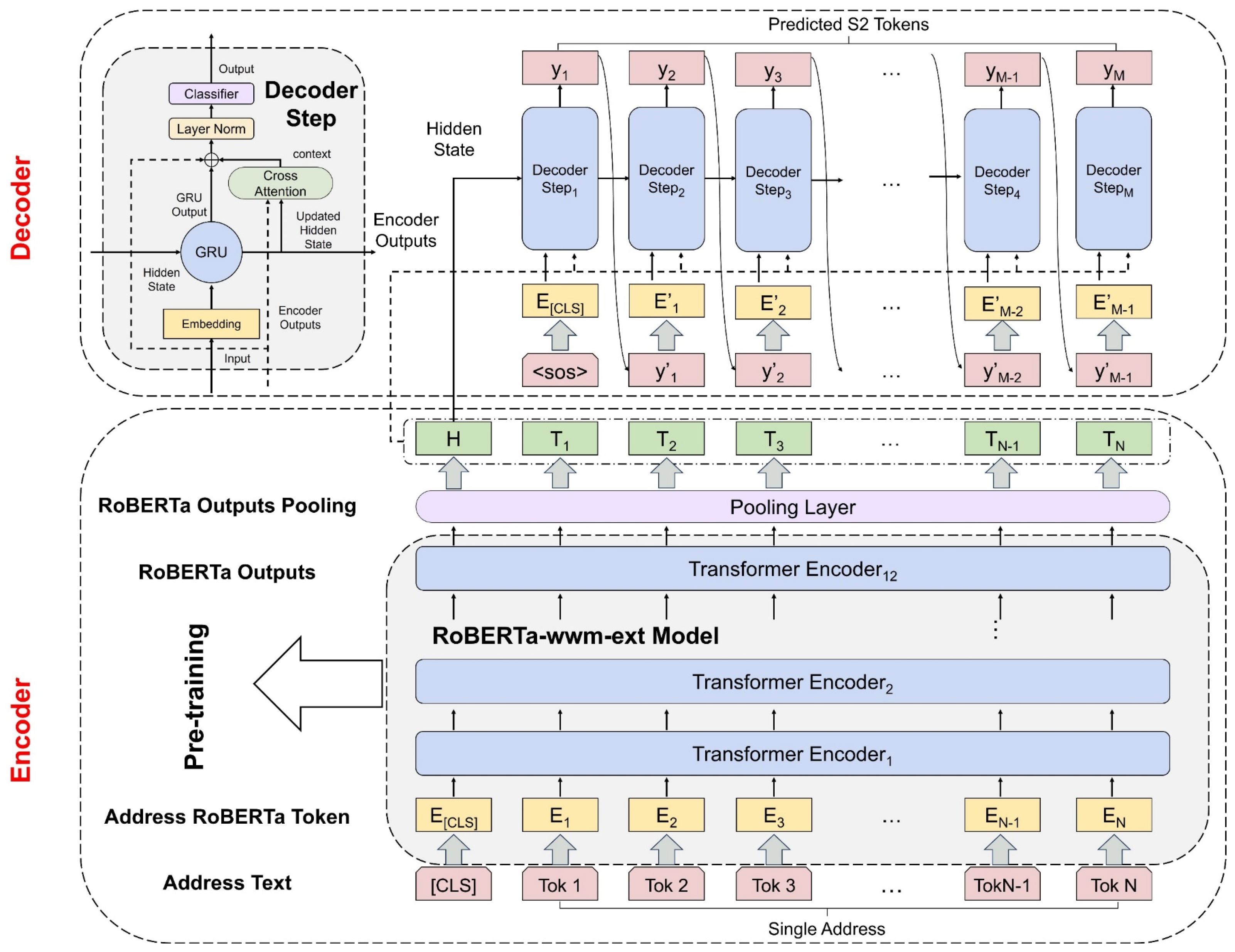
3.2. The Proposed Model Architecture
The HAGM consists of an encoder based on a pretrained language model and a decoder enhanced by a cross-attention mechanism. The encoder captures deep semantic features in the input text based on the pretrained RoBERTa language model, producing high-quality semantic representations. The decoder combines a recurrent neural network model with a cross-attention mechanism to perceive the hierarchical structure within the address text dynamically and accurately capture contextual information closely associated with the corresponding scale of the geographic grid. Additionally, the model adopts residual connections to preserve the original global context information and applies layer normalization to optimize performance. Finally, the processed combined information is transformed into a probability distribution matching the size of the target vocabulary through a linear classification layer, enabling character-by-character prediction of the S2 tokens. The model architecture is shown in
Figure 2, with detailed structures of the encoder and decoder described in
Section 3.2.1 and
Section 3.2.2, respectively.
3.2.1. Encoder
For the input address text, we designed a transformer-based encoder to capture rich semantic information within the input text and extract high-quality semantic representations. It was stacked with 12 transformer modules, each with hidden layer dimensions of 768. Every module integrates a multiheaded self-attention mechanism and a feed-forward neural network and applies layer normalization techniques. Using this structure, the model can perform deep feature extraction and semantic information capture from the input text, thereby providing a powerful feature extractor for downstream tasks. To better adapt to the characteristics of Chinese address text, we initialized the transformer-based encoder using the pretrained RoBERTa-chinese-wwm-ext model parameters [
52,
53], which utilizes the whole-word masking (wwm) strategy and is optimized on Chinese data. Furthermore, a fully connected layer was added after the output of the transformer-based encoder, projecting the feature vector dimensions from 768 to 512, which served as the input for the decoder.
Specifically, for an input query text, we first tokenized the text
into subword-level input representations
which were then fed into the pretrained RoBERTa model in order to obtain a deep representation of RoBERTa denoted as
.
Subsequently, we appended a fully connected layer to the end of the RoBERTa model for pooling, which compressed the dimensionality of the output from 768 to 512, thereby producing the final encoder output, denoted as
.
This helped the model to better compress, integrate, and transform the information from the input address text in order to adapt to the requirements of the decoder, optimize computational efficiency, and meet the needs of the downstream S2 encoding prediction task.
3.2.2. Cross-Attention-Enhanced Decoder
As mentioned in
Section 2, previous studies [
15,
29] have often overlooked the hierarchical characteristics of the address text and S2 tokens. To address this, we employed a cross-attention-enhanced recurrent neural network as the decoder, and a specific type of recurrent neural network was chosen as the gated recurrent unit (GRU) [
40]. With its gating mechanism, the GRU can effectively alleviate the problem of gradient disappearance and maintain long-term dependencies when dealing with long-term time series data. Thus, it performs well at capturing details and context relationships within address texts, surpassing traditional recurrent neural networks.
Specifically, the initial hidden state of the decoder is defined as
, where
refers to the vector representation of the first token “[CLS]” output by the encoder. We use the token “<sos>” as the initial input, denoted as
, and the update formula of GRU is:
To effectively capture the hierarchical relationship between address text elements and S2 tokens, we introduced a cross-attention mechanism into the decoder. While predicting each character by calculating the cross-attention scores between the current hidden state of the output sequence and various parts of the deep feature representations of the input address text sequence, the decoder dynamically weights the input address text, thus facilitating effective interaction between different modalities. This allows the model to focus dynamically on the most relevant hierarchical levels of address text elements at each character prediction step, thereby accurately capturing the contextual information closely associated with the corresponding scale of the geographic grid.
Specifically, for the current hidden state
, we compute the cross-attention weights
and the weighted context vector
with the semantic vectors
output by the encoder:
Given the characteristics of S2 tokens, the front characters of the sequence represent broader geographical scales, whereas the back characters tend to indicate finer scales. This makes it possible to precisely focus on the address element information of the corresponding hierarchical level when predicting characters at different positions of the S2 tokens. This mechanism enables effective information interaction between the input address text and output grid label sequence. Additionally, we effectively preserved the original global context information through residual connections, promoted efficient information transfer, and enhanced the model learning capability. By balancing local and global information, our model efficiently and comprehensively perceives the hierarchical structure of address texts and geographic grids, establishing a correspondence between address text elements at different hierarchical levels and geographic grids of varying scales.
Ultimately, the decoder needs to integrate the output of the GRU with the contextual information based on attentional weighting and transform it through a linear layer into a probability distribution equal to the size of the target vocabulary, thereby completing the character-by-character prediction of the S2 tokens.
Specifically, represents the probability distribution of the output classified as different S2 encoding characters at time step t, where (with including the 6 English letters a–f and 10 Arabic numerals 0–9), i.e., is a 16-dimensional probability vector. We define the predicted character of the final output based on as and simultaneously use it as the input for the next time step, denoted as . This process is repeated until a full S2 token sequence is generated, with the resulting sequence being represented as and the center of the S2 cell being used as the final predicted coordinate.
To ensure the robustness of the model and accelerate the training process, we introduced layer normalization (LN) [
54] before the final classification layer. The LN can normalize the input of each layer, thereby smoothing the flow of information and enhancing the robustness of the model.
3.3. Evaluation Metrics
We utilized four commonly used geocoding metrics to evaluate the model comprehensively: accuracy [
3] (also known as accuracy @N km), mean distance error, median distance error, and area under the curve (AUC) for the error curve [
55]. In this study, we first used the Haversine formula (a well-known method for calculating the geodetic distance between a pair of latitude and longitude points on an ellipsoidal Earth model) to calculate the great-circle distances between the predicted coordinates (
) and ground-truth coordinates (
), and then calculated each evaluation metric based on the obtained error distances.
Accuracy @N km measures the percentage of predicted locations that are less than N km from the true location. A higher percentage indicates that most predicted locations are within the allowable error threshold from the actual location, indicating that the model has higher precision in predicting geographical locations. Given the scope of this study, we set N to 0.05, which is equivalent to 50 m, because an error within 50 m can be considered relatively accurate. Although this metric is direct and straightforward, it disregards all errors exceeding 50 m.
Mean Distance Error measures the average distance between all predicted and true locations of the target address, and lower error values are preferred [
14]. It is calculated by dividing the sum of all the geocoding errors by their total number, revealing the overall performance of the geocoder and the general error trend. However, it is extremely sensitive to outliers, because it treats all errors as equivalent.
Median Distance Error measures the median distance between all the predicted locations and the true locations of the target address. Lower values are desired, signifying a greater alignment of the predictions with the true location. Compared to the mean distance error, the median distance error provides a more robust assessment of the performance of the geocoder because it is not affected by extreme errors.
AUC represents the area under the discrete curve of the sorted error distances, which serves as a significant comprehensive metric [
55] because it captures the overall distribution of errors and is not affected by outliers. The larger the AUC value, the more stable the performance of the geocoding model. In our study, the AUC was calculated using the logarithm of these distances, which shifted the focus of the metric towards smaller error distances when comparing models and reduced the importance of larger errors.
A versatile geocoding model should comprehensively consider all metrics in order to maximize performance [
6]. We further explored the performances and trends of the various models at different S2 levels.
4. Experiments and Results
4.1. Study Area and Dataset
We collected addresses from Dongcheng District, Beijing as the dataset for this study. Located in central Beijing, Dongcheng District covers an area of approximately 41.84 km2 and encompasses 17 streets and 177 communities. At the S2 level 20, this area contained 644,334 S2 cells. The original address dataset comprised 64,025 entries, covering various types of addresses, such as restaurants and shopping malls. Each entry includes detailed field information, such as place name, address description, longitude, latitude, and administrative divisions at various levels. We selected address descriptions containing rich geographical information as our input data. However, owing to irregularities in data entry and the variety of formats used, the quality and validity of the data vary; therefore, appropriate data processing is required.
To ensure the accuracy and consistency of the data, we conducted targeted preprocessing, which included: (1) identifying and removing duplicate and empty addresses in the dataset; (2) correcting invalid data, such as addresses with internal repetition or those containing special characters, full-width characters, or half-width characters; (3) combining the administrative division fields and name fields so as to randomly adjust address descriptions through supplementation, deletion, and concatenation, aiming to simulate query texts in real-world scenarios, and thereby increasing the diversity and practicality of address data. After preprocessing, we obtained 59,717 valid addresses, of which the longest address contained 82 tokens, and the average number of tokens for all addresses was 28.21. The text types considered in this study included completely hierarchically structured address descriptions and address descriptions with missing hierarchical elements. Some examples of address data are shown in
Table 2, in which some data lack elements such as cities, districts, streets, or roads, indicating that they are not standard hierarchical structured addresses.
We leveraged the S2 geometry to convert the geographic coordinates of each address description into the corresponding S2 tokens, serving as the ground truth for the addresses. Specifically, we utilized the Python package s2sphere to calculate the S2 cell grid labels (S2 Tokens) for each address. First, we converted the latitude and longitude coordinates of each address from degrees to radians. Subsequently, based on the converted radians, we identified the S2 cell at different levels that contained the given geographic location and calculated its corresponding grid ID. Finally, we converted the S2 cell ID into the corresponding S2 tokens and used them as the ground-truth label for the address. Thus, we completed the conversion of the output space, which satisfied the modeling requirements of the sequence-to-sequence analysis. Finally, we split the preprocessed 59,717 labeled valid address data in a 9:1 ratio. The training set contained 90% of the data and was dedicated to model training. The remaining 10% of the data served as the test set to evaluate the model’s performance.
4.2. Training and Experimental Setup
4.2.1. Training Details
During the training process, the input of our model was the preprocessed address description, the output was the predicted sequence of S2 tokens, and the corresponding truth labels were the sequences of S2 tokens previously computed from the latitude and longitude labels of the address text. The predicted output of each sequence character was a 16-dimensional vector of probability distributions, as shown in
Figure 1b. We selected the character with the highest probability at each prediction step as the final output for that time step and used it as the input of the next time step. For each time step, we computed the cross-entropy loss between the probability distributions of the characters predicted by the model and the real characters, summing the losses of all time steps to obtain the total loss. By minimizing the total loss, we can optimize the model parameters to better understand the relationship between the input and output sequences. Additionally, during the training, we employed a teacher-forcing strategy. This strategy involved using true sequence characters as inputs for the next time step with a certain probability, rather than relying solely on the model’s predicted results. This approach helped increase the robustness of the sequence-to-sequence model and accelerated the convergence process of the model. The total loss was calculated using the following equation:
Our model was trained on a single NVIDIA GeForce RTX 3090 GPU with a memory of 24 GB using the PyTorch framework. To better handle the difference in structural complexity between the encoder and decoder, we set different learning rates: the learning rate for the encoder was set to 1 × 10
−5, and the learning rate for the decoder was set to 7 × 10
−4. After the initial warm-up phase, the learning rate decayed exponentially with an increase in batches, which helped stabilize the training process of the model. Throughout the training process, we used the Adam optimizer for stable parameter updates, processing 64 samples per training batch, and training the model for a total of 200 epochs. Adam is an algorithm used for optimizing gradient descent. This algorithm is especially suitable for dealing with sparse gradients and adaptively adjusting the learning rate and can effectively improve the efficiency of deep learning model training [
56]. To improve the generalizability of the model and prevent overfitting, we introduced dropout technology and set it to 0.5.
4.2.2. Experimental Setup
To compare the performance of our model with other geocoding models, we selected the SLG [
29] (single-level geocoding), MLG [
29] (multi-level geocoding), and MLSG [
14] (multi-loss geocoding) models as baselines to evaluate the strengths and improvements of our proposed model in fine-grained geocoding tasks. These models are representative of different processing strategies and design ideas for geocoding tasks in recent years. Among them, the SLG model is the most basic grid-based classification geocoding method. The MLG model mitigates the problem of growing output spatial dimensionality by combining multilevel grids, and the MLSG model demonstrates another way to cope with the spatial complexity of high-dimensional outputs by combining the classification loss with the coordinate regression loss. All of these methods employed RoBERTa to obtain feature representations from the input address and aimed to predict the corresponding grid label and coordinates under the S2 partition as their shared objective in order to ensure consistent evaluation.
Moreover, to evaluate our model comprehensively, we categorized the study area into sparse regions (less than 2), dense regions (more than 10), and regular regions (between 2 and 10) based on the number of address data entries within the unit area. We evaluated the performance metrics for each of these regions as well as the overall region to verify the consistency and accuracy of the model for various geographical data distributions. We also assessed the accuracy and generalization of the model at all levels, from 15 to 20, to explore its performance at different spatial granularities, thereby determining the optimal scale for geocoding. Additionally, we explored the model performance in fine-grained geocoding tasks by setting N in the Accuracy@N km metric to 10, 25, and 50.
To explore the effectiveness of the model and the contribution of each component, we conducted ablation experiments on key modules, including the cross-attention mechanism and layer normalization. Furthermore, to enable meaningful comparisons with the method in [
48], we focused on core module differences, given our adoption of more advanced backbone and grid partitioning techniques, along with the integration of residual connections and layer normalization modules. Specifically, we replaced the HGAM’s cross-attention module with the self-attention module used in [
40] to achieve a fair comparison. In this way, we can analyze the respective contributions of each module to the model performance, allowing for a more comprehensive and objective evaluation of our model.
4.3. Results
We evaluated the performances of SLG, MLG, MLSG, and our model across different density distribution areas and various S2 levels for all metrics. All of the results of the comparison models were based on our own implementation, and training and testing were conducted under the same environment and dataset to ensure the fairness of the experiments.
4.3.1. Overall Trends
As shown in
Table 3,
Table 4 and
Table 5, our model demonstrated a significant advantage across all evaluation metrics compared to SLG, MLG, and MLSG. The AUC metric of our model reached its highest value at 0.59, surpassing the values achieved by SLG, MLG, and MLSG by 4, 5, and 6 percentage points, respectively, implying that our model had an excellent overall error distribution that tended towards lower error values. The median distance error of our model was as low as 41.46 m, which is at least 6 m better than that of the other models. For the more stringent metric, Accuracy@50m, our model scored up to 0.56, which is an improvement of at least 4 percentage points compared to other models, suggesting that most of the predictions of our model are quite accurate. Moreover, the mean distance error metric of our model was 93.98 m, outperforming SLG, MLG, and MLSG by approximately 31 m, 26 m, and 8 m, respectively. This implies that our model maintains good predictive quality in most scenarios, demonstrating its resilience to noise and robustness. As shown in
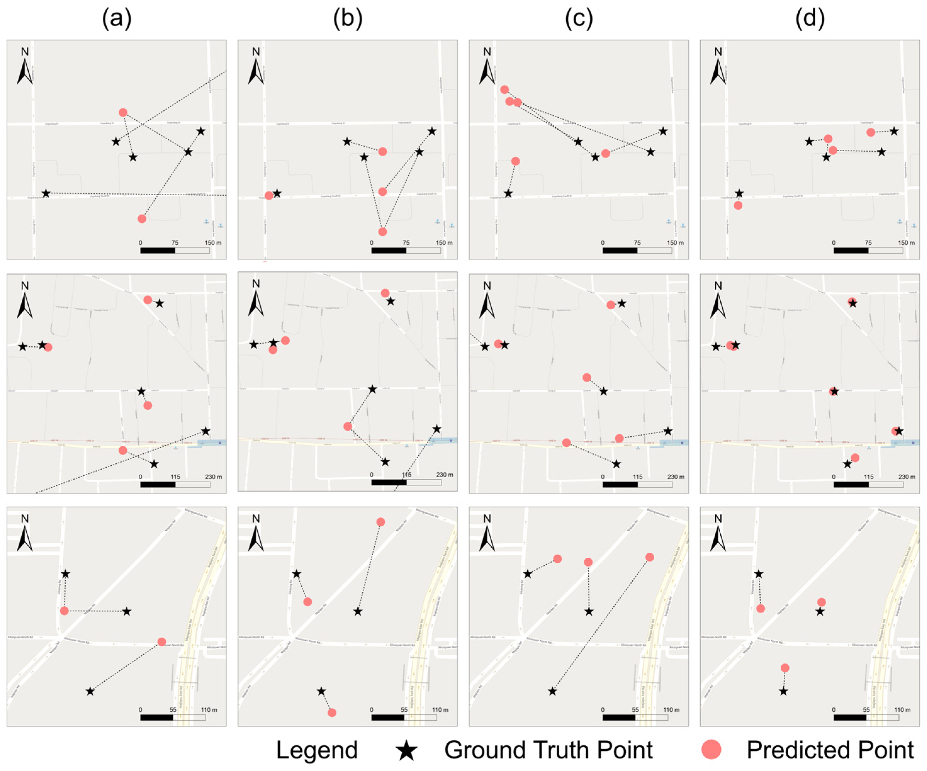
Figure 3, the predicted results of our model closely matched the actual distribution in most regions with smaller distance errors.
Furthermore, our HAGM model achieved the best accuracy when the S2 level was set to 20, whereas the other models peaked at S2 levels of 17 or 18. As shown in
Table 5, at L20, our model surpassed the baseline models by at least 3 percentage points on the AUC and outperformed comparative models by a minimum of 9 percentage points on the Accuracy@50m dataset. Meanwhile, the median and mean distance errors of our model were reduced by at least 13.72 m and 30.42 m, respectively. As shown in
Table 4, our model achieved the best results for the Accuracy@10m, Accuracy@25m, and Accuracy@50m metrics. This suggests that when the output space features more detailed and refined grid partitioning, the HAGM can successfully learn more granular spatial information than the other models, making it better suited for learning fine-grained geocoding tasks.
In summary, our model demonstrates a more comprehensive and balanced performance with significant advantages, which is in line with the standards of a versatile geocoder.
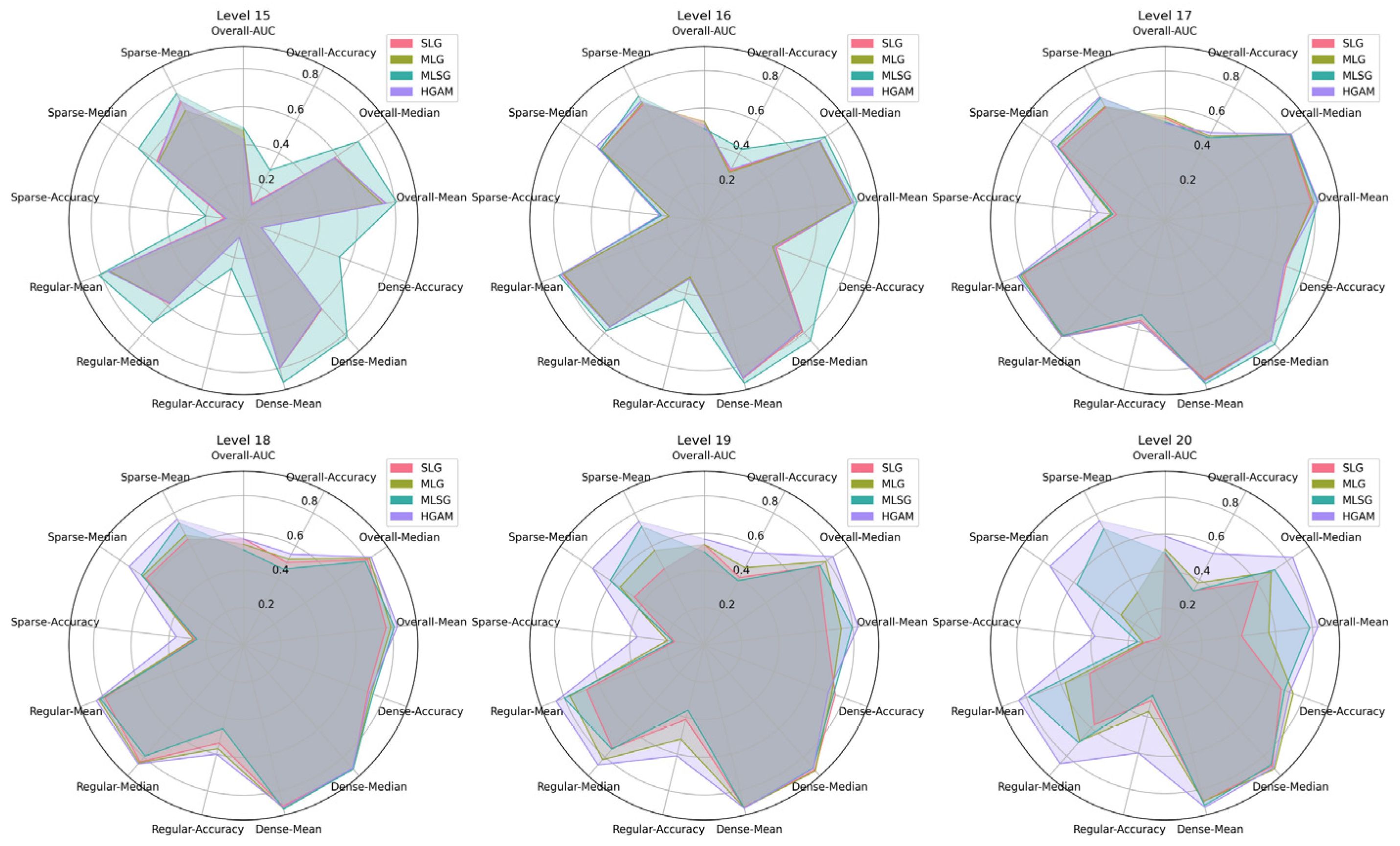
Table 5 and
Figure 4 provide a detailed presentation of the performance of the model at different S2 levels and in regions with varying data distributions; a deeper analysis and discussion will be carried out in the subsequent sections.
4.3.2. Performance across Different S2 Levels
To explore the performance of the models at various spatial partitioning scales, we evaluated the accuracy of each model at the S2 levels 15–20. As shown in
Figure 4 and
Table 5, the accuracy of SLG, MLG, and MLSG initially showed an increasing trend as the S2 level increased but started to decline after reaching an optimum between L17 and L18. Meanwhile, HAGM demonstrated weaker performance at L15 and L16, but steadily improved as the S2 level increased, surpassing other models and peaking at L20. This suggests that the HAGM can learn granular spatial information more effectively and handle high-resolution geospatial data.
As the S2 level increases, the granularity of the output space partitioning becomes even more refined, leading to a sharp increase in the number of S2 cells within the study area; thus, traditional classification models such as SLG, MLG, and MLSG face the problem of dimensionality explosion in the output space, which leads to a decrease in accuracy. Although MLG and MLSG have attempted to mitigate this issue by fusing the results from multiple levels or adopting weighted predictions, their performance still suffers at finer scales, such as L19 and L20. By contrast, HAGM adopts a character-by-character prediction strategy in which each character’s prediction involves only a 16-dimensional output space, and, thus, effectively avoids this problem and successfully gathers knowledge at finer scales.
4.3.3. Performance across Different Area Densities
To explore the performance of the models across varying data distribution regions, we assessed the precision of each model in the sparse, regular, dense, and overall regions. As shown in
Table 5 and
Figure 4, all of the models exhibited substantially lower performance metrics in sparse and regular regions than in dense regions. This difference can be attributed to the higher data density in denser regions, which provides the model with more opportunities to capture geospatial patterns. By contrast, sparse regions have a more scattered data distribution, causing the model to be easily influenced by dense regions and thereby leading to bias, which is also consistent with the view expressed in [
29].
Specifically, as shown in
Figure 4, as the level increased beyond the respective optimal S2 level, the performance indicators in the dense regions for the baseline models did not decline severely. However, at the same time, there is a significant decline in performance in sparse and regular regions, as observed in the performance of MLG and MLSG at L18, L19, and L20 in sparse and regular regions, which ultimately impacts the model’s overall performance. This suggests that the underperformance of geocoders based on grid prediction methods in high-precision geocoding tasks may stem from their inadequacy when learning from sparse regions.
In contrast, our model shows significant advantages in both sparse and regular regions while maintaining good performance in dense regions. Particularly at L20, the Accuracy@50m of our model achieves 0.38 in sparse regions, an improvement of at least 9 percentage points compared to other models, while the median and mean metrics reach 66.27 m and 142.79 m, respectively, a reduction of 16.27 m and 7.52 m. These figures indicate that our model can effectively learn geospatial distribution patterns even in sparse regions with strong generalization and stability across different data distributions. This advantage may be related to the strategy of our model, which tends to learn a pattern of mapping from address elements of different hierarchical levels to the corresponding S2 tokens characters. Therefore, even in sparse regions, our model can apply the knowledge of spatial hierarchies learned from other regions, partially reducing the impact of the data distribution density and achieving relatively good accuracy.
4.3.4. Performance across Various Address Types
To explore the performance of the models across different data types, we evaluated each model for complete and incomplete address descriptions with missing elements. The results indicate that our model outperformed the other models for both address types. In particular, as shown in
Table 6, our model achieved the best median and mean distance errors in incomplete address descriptions, reducing at least 6.30 m and 27.15 m compared to the baseline model. Moreover, it showed a significant advantage, with a 4-percentage-point increase in the AUC metric, compared with that of the other models. Owing to the limited information in incomplete address descriptions, all models showed a decrease in performance for incomplete address descriptions compared with complete address descriptions. However, the HGAM exhibited markedly lesser performance degradation for incomplete address descriptions, significantly outperforming the baseline model. Specifically, the mean distance error of the HGAM increased by only 24.28 m, whereas the average distance errors of the baseline models SLG, MLG, and MLSG increased by 51.46 m, 39.31 m, and 44.54 m, respectively. In addition, the median distance error of HGAM increased by only 1.88 m compared to the full address description. This indicates that the proposed model is more robust. By considering both local and global information, it can better cope with missing elements and maintain a relatively good performance even in cases of insufficient information.
4.3.5. Ablation Study
As shown in
Table 7, incorporating the cross-attention (CA) mechanism resulted in a 3-percentage-point improvement in both the AUC and Accuracy@50m metrics of our model and reductions of 3.87 m and 3.42 m in the median and mean distance errors, respectively. Introducing the layer normalization mechanism led to a 2-percentage-point improvement in both the AUC and Accuracy@50m metrics and reductions of 1.44 m and 2.16 m to the median and mean distance errors, respectively. Additionally, compared to the self-attention (SA) module, using the cross-attention (CA) module improved the AUC and Accuracy@50m metrics for our model by 1 and 2 percentage points, respectively, and reduced the median and mean distance errors by 2.73 m and 3.01 m, respectively. These results demonstrate the effectiveness and superiority of the cross-attention and layer normalization modules.
The cross-attention mechanism enables the model to dynamically perceive and focus on different elements of the address text, thereby accurately capturing the contextual information of the corresponding geographical scale. This enhances the prediction precision by establishing a correspondence between the input address text elements and geographic grids across different scales. The model focuses on large-scale textual description features (e.g., provinces) when predicting characters at the front of the sequence and focuses on finer-scale textual geographic information features (e.g., specific buildings) when predicting characters at the back of the sequence, which matches the hierarchical structure of the address text.
The LN module not only accelerates the training process of the model through the layer normalization process but also provides stability and avoids gradient explosion or vanishing of the model during the training process, which further improves the robustness and prediction accuracy of the model.
4.4. Discussion
In summary, SLG exhibited the lowest performance metrics in all aspects; MLSG stood out in the mean distance error but was relatively weaker in AUC, median distance error, and Accuracy@50m; and MLG performed well in Accuracy@50m and median distance error but fell short in mean distance error. By contrast, our model performed best in all four evaluation metrics—AUC, Accuracy@50m, mean distance error, and median distance error—demonstrating a well-balanced performance.
Compared with the simple single-level geocoding model (SLG), both MLG and MLSG demonstrate partial performance improvements. MLG integrates the classification results of multi-level grids, which, to some degree, mitigates dimensionality explosion and shows enhanced performance in sparse regions. MLSG combines classification and coordinate regression losses and derives the final prediction coordinates by weighting the classification results, which enhances its robustness. However, they still have limitations because their accuracies decrease at finer spatial partitioning scales.
In contrast, our model achieved the best performance for all four metrics, demonstrating a more comprehensive performance. Moreover, it is worth noting that our model has significant advantages in sparse and regular regions, as shown in
Table 5 and
Figure 4. Taking the evaluation results at level 20 as an example, in sparse and regular regions, HGAM reduced the metric of median distance error by at least about 52 m and 44 m, respectively, compared to other models. Moreover, it showed an increase of at least 23 percentage points in the Accuracy@50m metric compared to the other models. It adopts a sequence-to-sequence approach to predict S2 tokens character by character, which leans towards learning the mapping patterns from specific elements of the text to the corresponding S2 token characters. By integrating the cross-attention and residual connection module, it learns the hierarchical structure of the address text and the output S2 token sequence in more detail in order to establish the correspondence between address text elements at different hierarchical levels and geospatial grids of varying scales. This ensures that the prediction of different locations of S2 tokens dynamically focuses on the corresponding geographical scale information rather than simply predicting the entire grid label category based on the address text as a whole.
Although our model shows good performance, these deep learning methods, including ours, often require new pretraining or fine-tuning in unknown regions, which may lead to increased geocoding costs. In the future, we will expand our study area and explore efficient fine-tuning methods to reduce the construction costs of geocoding models.


