

Agent-Based Modeling of COVID-19 Transmission: A Case Study of Housing Densities in Sankalitnagar, Ahmedabad


Abstract
:1. Introduction
2. Study Area
3. Methods
3.1. Housing Density Classification
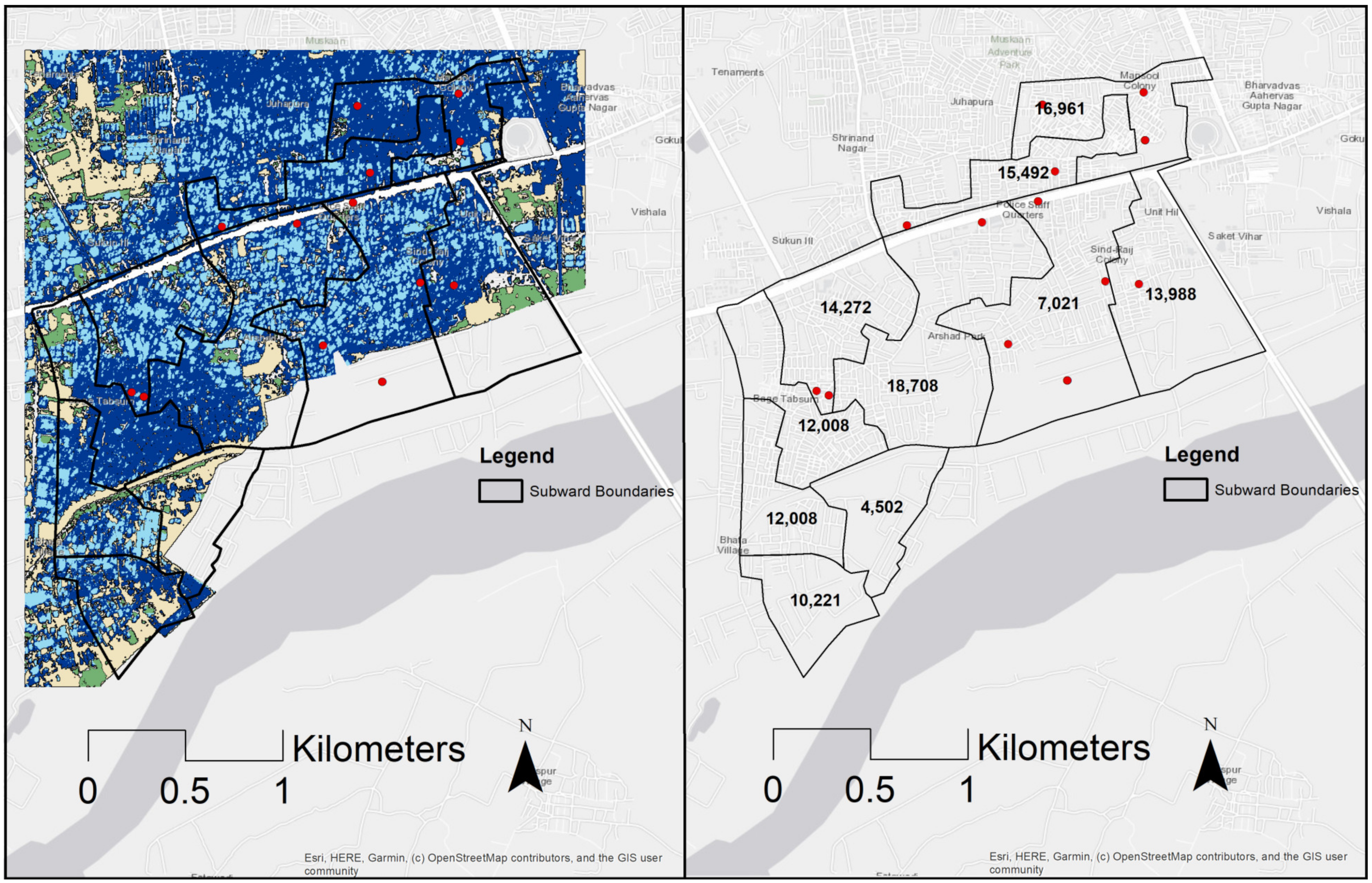
3.2. Population Density Estimations for Sankalitnagar
3.3. Agent-Based Modeling (ABM) of COVID-19
3.3.1. Agents
3.3.2. Modeling Interface
3.3.3. Environment
3.3.4. Agent Movement
3.3.5. Disease Transmission
3.3.6. Initialization and Verification
4. Results
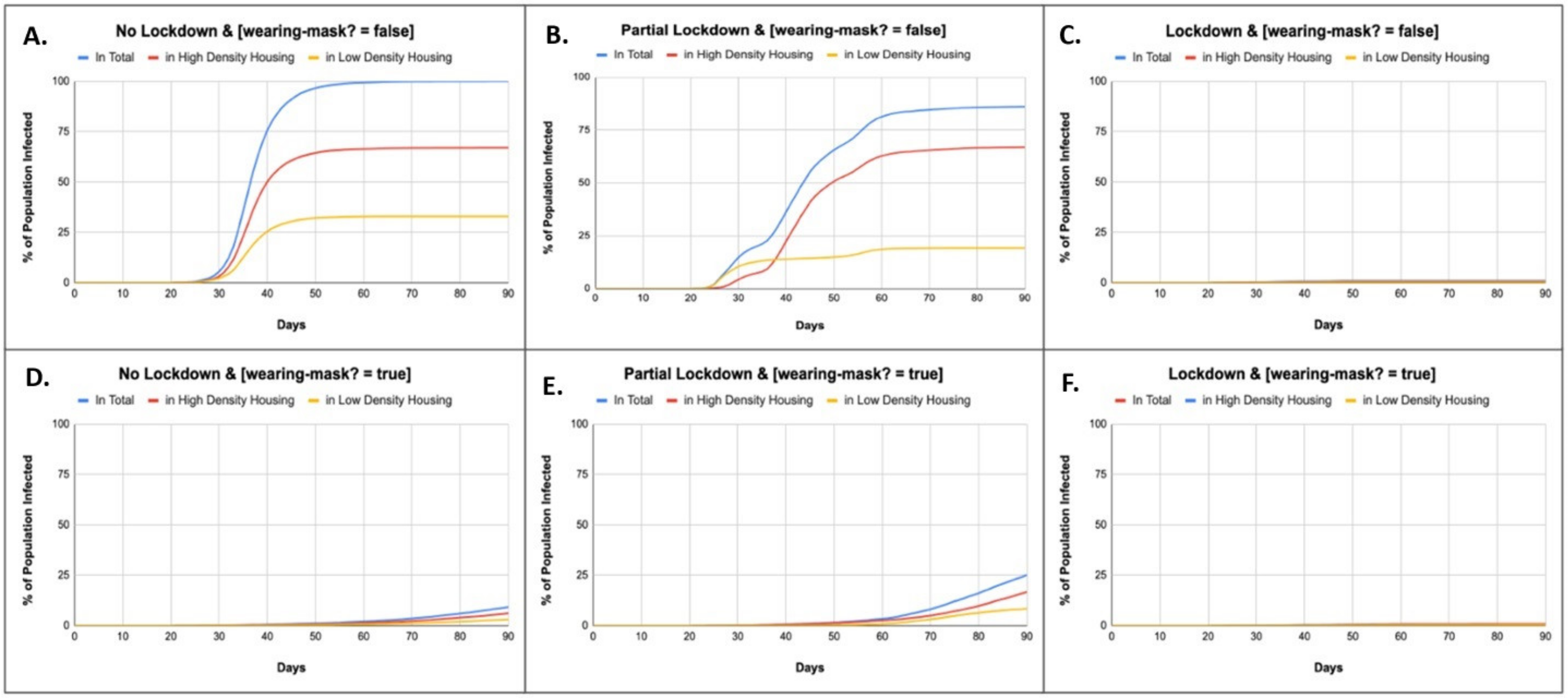
4.1. Model Runs
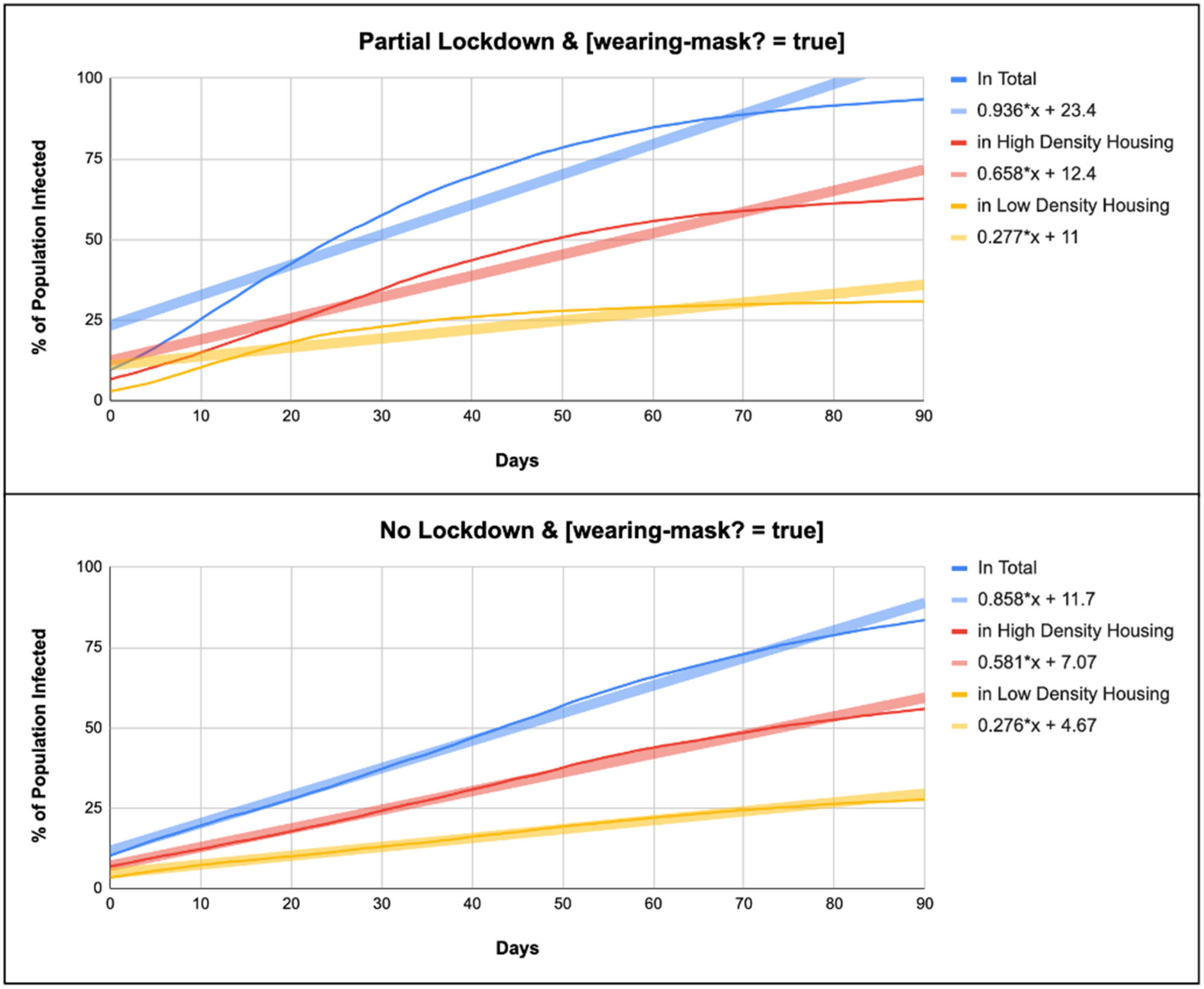
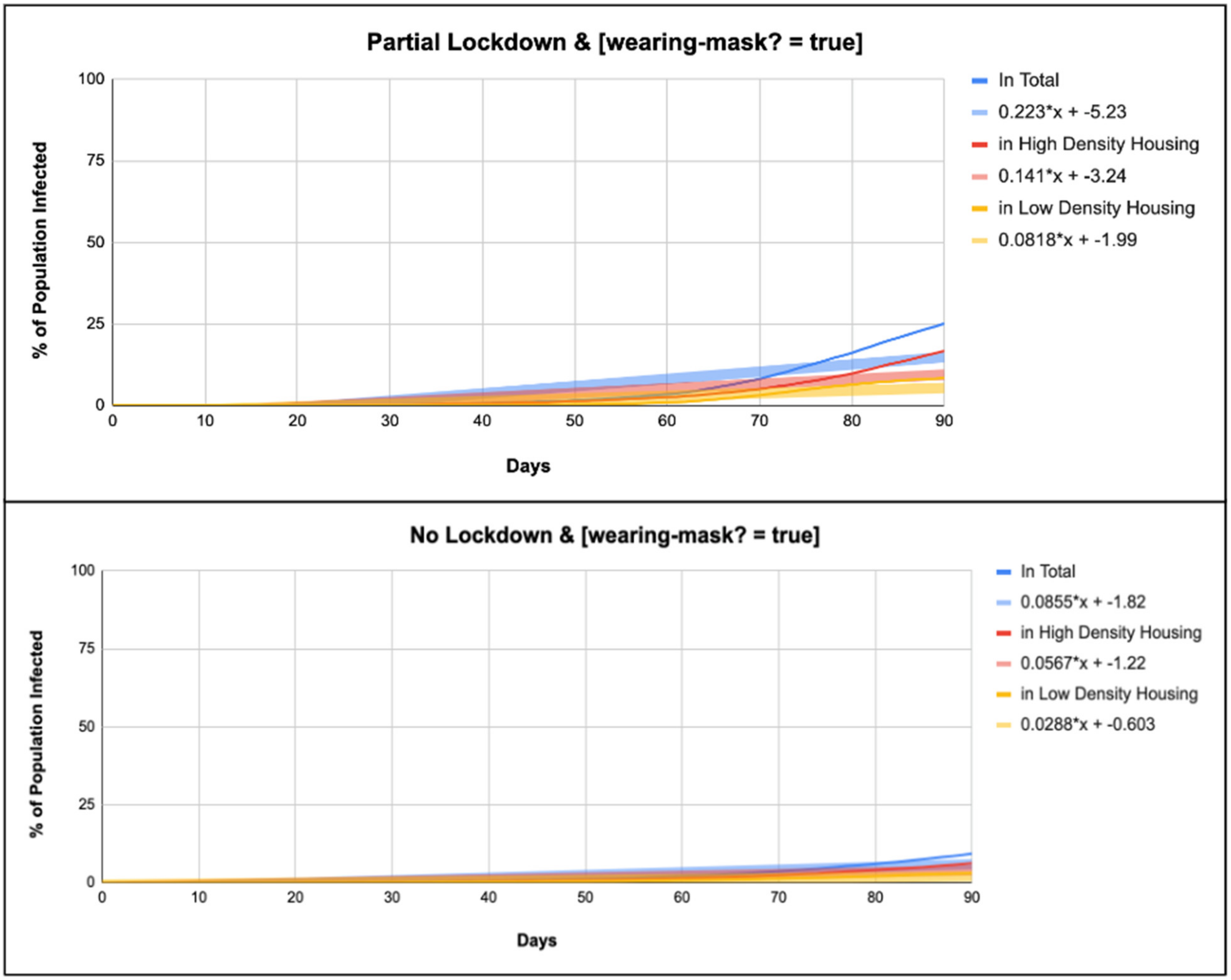
4.2. Variation in Model Output
5. Limitations and Future Work
6. Discussion and Conclusions
Author Contributions
Funding
Institutional Review Board Statement
Data Availability Statement
Conflicts of Interest
Appendix A. Netlogo Source Code
| ;SETUP ---------------------------------------------------------------------- |
| extensions [gis profiler] |
| breed [low lows] |
| breed [high highs] |
| breed [sick sicks] |
| globals[ |
| ;globals representing datasets |
| housing |
| buffer |
| cases |
| density |
| buffer-coords |
| boundary |
| ;global representing ticks |
| counter |
| ;globals representing patches |
| high-patches |
| low-patches |
| neighborhood-patches |
| boundary-patches |
| high-density-turtles |
| low-density-turtles |
| ] |
| patches-own[ |
| high-density? |
| low-density? |
| patch-ID |
| ] |
| turtles-own [ |
| origin |
| origin-xy |
| origin-x |
| origin-y |
| origin-patch |
| sick? |
| recovered? |
| symptomatic? |
| infected? |
| infectious? |
| origin-ID |
| exposure-date |
| sick-duration |
| incubation |
| high-density-t? |
| low-density-t? |
| ] |
| to load-data |
| __clear-all-and-reset-ticks ;clear remains of previous runs |
| load-housing |
| load-features |
| gis:set-world-envelope (gis:envelope-union-of (gis:envelope-of boundary) |
| (gis:envelope-of buffer) |
| (gis:envelope-of cases) |
| (gis:envelope-of housing)) |
| set counter 0 |
| end |
| to load-features |
| set boundary gis:load-dataset “Shapefile_Simplified_Density.shp” |
| set buffer gis:load-dataset “Shapefiles_1kmbuffer.shp” |
| set cases gis:load-dataset “CovidCases_1kmbuffer.shp” |
| end |
| to load-housing |
| set housing gis:load-dataset “ml_1_arcmap_gcs.asc” |
| ;gis:load-coordinate-system “/Users/mollyfrench/Desktop/Sankalitnagar Model/FINAL MODEL_1/FINAL MODEL/Data/Shapefiles from Dr. Quereshi/Shapefile_Simplified.prj” |
| end |
| ;HOUSING ---------------------------------------------------------------------- |
| to apply-housing |
| ;resize-world 0 gis:width-of (housing) 0 gis:height-of (housing) |
| gis:apply-raster housing density |
| ;resize-world 0 gis:width-of (housing) 0 gis:height-of (housing) |
| ask patches [ |
| set density gis:raster-sample housing self |
| if (density = 42)[ |
| set high-density? true |
| set pcolor 48 |
| ] |
| if (density = 53) [ |
| set low-density? true |
| set pcolor 98 |
| ] |
| ] |
| end |
| to sample-housing |
| ask patches [ |
| set density gis:raster-sample housing self |
| if (density = 42)[ |
| set high-density? true |
| set pcolor 48 |
| ] |
| if (density = 53) [ |
| set low-density? true |
| set pcolor 98 |
| ] |
| ] |
| end |
| ;SETUP POPULATION ---------------------------------------------------------------------- |
| to apply-population-evenly |
| set boundary-patches (patches gis:intersecting boundary) |
| foreach gis:feature-list-of boundary [ |
| neighborhood -> |
| ;Get the population for a high density neighborhood, take 2/3 of population |
| ;FOR NOW DIVIDE BY 100 AND ROUND |
| let high-density-pop round ((gis:property-value neighborhood "HIGH_POP") / 10) |
| let low-density-pop round ((gis:property-value neighborhood "LOW_POP") / 10) |
| let neighborhood-pop round ((gis:property-value neighborhood "POP") / 10) |
| set neighborhood-patches (patches gis:intersecting neighborhood) with [gis:contained-by? self neighborhood] |
| ask neighborhood-patches [set patch-ID gis:property-value neighborhood “Id”] |
| set high-patches (patches gis:intersecting neighborhood) with [gis:contained-by? self neighborhood] with [high-density? = true] |
| set low-patches (patches gis:intersecting neighborhood) with [gis:contained-by? self neighborhood] with [low-density? = true] |
| ;ask high-patches [set pcolor white] |
| ask n-of high-density-pop high-patches[ |
| sprout-high 1[ |
| set origin patch-here |
| set origin-ID patch-ID |
| set infected? false |
| set recovered? false |
| set high-density-t? true]] |
| ask n-of low-density-pop low-patches[ |
| sprout-low 1[ |
| set origin patch-here |
| set origin-ID patch-ID |
| set infected? false |
| set recovered? false |
| set low-density-t? true]] |
| ] |
| end |
| to setup-infected-within-buffer |
| ;if ticks = 0 ;;[set dt time:create “2020/3/17 00:00”] |
| ;[show “Showing Covid19 Cases from 17/3/2020...”] |
| foreach gis:feature-list-of cases [ vector-feature -> let day gis:property-value vector-feature “Days_Since” |
| if day = counter |
| [let starting-point gis:location-of(gis:centroid-of(vector-feature)) |
| ;set up so there is 2/3 chance that sick is part of high-density population and 1/3 chance that sick is part of low-density population |
| if-else (random-float 100 < 67) |
| [create-high 1[ |
| set size 5 |
| set color blue |
| set xcor (item 0 starting-point) |
| set ycor (item 1 starting-point) |
| set origin one-of boundary-patches with [high-density? = true] |
| set origin-ID [patch-ID] of origin |
| set high-density-t? true |
| set exposure-date counter |
| set sick-duration 2 + (random 12) ;set incubation period between 2–14 days |
| set infected? true |
| set recovered? false]] |
| [create-low 1[ |
| set size 5 |
| set color blue |
| set xcor (item 0 starting-point) |
| set ycor (item 1 starting-point) |
| set origin one-of boundary-patches with [low-density? = true] |
| set origin-ID [patch-ID] of origin |
| set low-density-t? true |
| set exposure-date counter |
| set sick-duration 2 + (random 12) ;set incubation period between 2–14 days |
| set infected? true |
| set recovered? false]] |
| ] |
| ] |
| ;set counter counter + 1 |
| ;ifelse ticks = 50 |
| ;[stop] |
| end |
| to setup-sick-populations |
| ask turtles [ |
| if (random-float 100 < %-population-infected-at-start)[ |
| set exposure-date counter |
| set sick-duration 2 + (random 12) ;set incubation period between 2–14 days |
| set infected? true |
| set recovered? false]] |
| end |
| ;TO MODEL |
| to clear |
| __clear-all-and-reset-ticks |
| set counter 0 |
| end |
| to setup |
| __clear-all-and-reset-ticks |
| set counter 0 |
| load-data |
| sample-housing |
| apply-population-evenly |
| if inital-sick-population = “random population” [setup-sick-populations] |
| ask turtles [ |
| set size 5 |
| set shape “person”] |
| end |
| to run-model |
| ;setup initial sick population when setting up model |
| if inital-sick-population = “from government data” [ |
| setup-infected-within-buffer] |
| ;1) have turtles move according to scenario |
| if scenario = “No Lockdown”[ |
| ask turtles with [high-density-t? = true] [ |
| move-to one-of patches with [patch-ID = [origin-ID] of myself] |
| ] |
| ask turtles with [low-density-t? = true] [ |
| move-to one-of boundary-patches] |
| ] |
| if scenario = “Partial Lockdown”[ |
| ask turtles with [high-density-t? = true] [ |
| move-to one-of patches with [(patch-ID = [origin-ID] of myself) AND (high-density? = true)] |
| ] |
| ask turtles with [low-density-t? = true] [ |
| move-to one-of patches with [patch-ID = [origin-ID] of myself AND (low-density? = true)]] |
| ] |
| if scenario = “Lockdown”[ |
| ask turtles with [high-density-t? = true] [ |
| stop |
| ] |
| ask turtles with [low-density-t? = true] [ |
| stop] |
| ] |
| ;2) after turtles move- ask them to infect one another or catagorize themselves |
| ask turtles [ |
| if (infected? = true) ;AND (recovered? = false) |
| [ |
| infect] |
| if (infected? = true) AND (counter = exposure-date + sick-duration) [ |
| set recovered? true] |
| ] |
| ;3) have turtles return home in the evening |
| ask turtles [ |
| move-to origin] |
| ;4) ask turtles to re-infect at home |
| ask turtles [ |
| if (infected? = true) AND (recovered? = false)[ |
| infect]] |
| set counter counter + 1 |
| tick |
| end |
| ;COVID-19 DISEASE SPREAD--------------------------------------------------------------- |
| to infect |
| let nearby-uninfected (turtles-on neighbors) with [infected? = false] |
| if any? nearby-uninfected [ |
| ask nearby-uninfected [ |
| if wearing-mask? = true [ |
| if random-float 100 <= 7 [ |
| set exposure-date counter |
| set sick-duration 2 + (random 12) ;set sick period between 2–14 days |
| set infected? true |
| set recovered? false |
| ]] |
| if wearing-mask? = false [ |
| if random-float 100 <= 52 [ |
| set exposure-date counter |
| set sick-duration 2 + (random 12) ;set sick period between 2–14 days |
| set infected? true |
| set recovered? false |
| ] |
| ]]] |
| end |
References
- Crooks, A.T.; Hailegiorgis, A.B. An agent-based modeling approach applied to the spread of cholera. Environ. Model. Softw. 2014, 62, 164–177. [Google Scholar] [CrossRef]
- Marques, J.; Cezaro, A.; Lazo, M.J. A SIR Model with Spatially Distributed Multiple Populations Interactions for Disease Dissemination. Trends Comput. Appl. Math. 2022, 23, 143–154. [Google Scholar] [CrossRef]
- Goel, R.; Sharma, R. Mobility based SIR model for pandemics-with case study of COVID-19. In Proceedings of the 2020 IEEE/ACM International Conference on Advances in Social Networks Analysis and Mining (ASONAM), The Hague, The Netherlands, 7–10 December 2020; pp. 110–117. [Google Scholar]
- Goel, R.; Bonnetain, L.; Sharma, R.; Furno, A. Mobility-based SIR model for complex networks: With case study of COVID-19. Soc. Netw. Anal. Min. 2021, 11, 105. [Google Scholar] [CrossRef] [PubMed]
- Kong, L.; Duan, M.; Shi, J.; Hong, J.; Chang, Z.; Zhang, Z. Compartmental structures used in modeling COVID-19: A scoping review. Infect. Dis. Poverty 2022, 11, 72. [Google Scholar] [CrossRef] [PubMed]
- Dunham, J.B. An agent-based spatially explicit epidemiological model in MASON. J. Artif. Soc. Soc. Simul. 2005, 9, 3. [Google Scholar]
- Miksch, F.; Jahn, B.; Espinosa, K.J.; Chhatwal, J.; Siebert, J.; Popper, N. Why should we apply ABM for decision analysis for infectious diseases?—An example for dengue interventions. PLoS ONE 2019, 14, e0221564. [Google Scholar] [CrossRef] [PubMed]
- Willem, L.; Verelst, F.; Bilcke, J.; Hens, N.; Beutels, P. Lessons from a decade of individual-based models for infectious disease transmission: A systematic review (2006–2015). BMC Infect. Dis. 2017, 17, 612. [Google Scholar] [CrossRef] [PubMed]
- Anderson, T.; Dragićević, S. NEAT approach for testing and validation of geospatial network agent-based model processes: Case study of influenza spread. Int. J. Geogr. Inf. Sci. 2020, 34, 1792–1821. [Google Scholar] [CrossRef]
- Bian, L. A Conceptual Framework for an Individual-Based Spatially Explicit Epidemiological Model. Environ. Plan. B Plan. Des. 2004, 31, 381–395. [Google Scholar] [CrossRef]
- Perez, L.; Dragicevic, D. An agent-based approach for modeling dynamics of contagious disease spread. Int. J. Health Geogr. 2009, 8, 50. [Google Scholar] [CrossRef]
- Hoertel, N.; Blachier, M.; Blanco, C.; Olfson, M.; Massetti, M.; Rico, M.S.; Limosin, F.; Leleu, H. A stochastic agent-based model of the SARS-CoV-2 epidemic in France. Nat. Med. 2020, 26, 1417–1421. [Google Scholar] [CrossRef]
- Paez, A.; Lopez, F.A.; Menezes, T.; Cavalcanti, R.; Galdino da Rocha Pitta, M. A spatio-temporal analysis of the environmental correlates of COVID-19 incidence in Spain. Geogr. Anal. 2021, 53, 397–421. [Google Scholar] [CrossRef]
- Manout, O.; Ciari, F. Assessing the role of daily activities and mobility in the spread of COVID-19 in Montreal with an agent-based approach. Front. Built Environ. 2021, 7, 654279. [Google Scholar] [CrossRef]
- Liu, J.; Ong, G.P.; Pang, V.J. Modelling effectiveness of COVID-19 pandemic control policies using an Area-based SEIR model with consideration of infection during interzonal travel. Transp. Res. Part A Policy Pract. 2022, 161, 25–47. [Google Scholar] [CrossRef]
- Tribby, C.P.; Hartmann, C. COVID-19 cases and the built environment: Initial evidence from New York City. Prof. Geogr. 2021, 73, 365–376. [Google Scholar] [CrossRef]
- von Seidlein, L.; Alabaster, G.; Deen, J.; Knudsen, J. Crowding has consequences: Prevention and management of COVID-19 in informal urban settlements. Build. Environ. 2021, 188, 107472. [Google Scholar] [CrossRef]
- Bhadra, A.; Mukherjee, A.; Sarkar, K. Impact of population density on COVID-19 infected and mortality rate in India. Model. Earth Syst. Environ. 2021, 7, 623–629. [Google Scholar] [CrossRef] [PubMed]
- Kanga, S.; Meraj, G.; Sudhanshu; Farooq, M.; Nathawat, M.; Singh, S. Analyzing the risk to COVID-19 infection using remote sensing and GIS. Risk Anal. 2021, 41, 801–813. [Google Scholar] [CrossRef]
- Glodeanu, A.; Gullón, P.; Bilal, U. Social inequalities in mobility during and following the COVID-19 associated lockdown of the Madrid metropolitan area in Spain. Health Place 2021, 70, 102580. [Google Scholar] [CrossRef]
- Kerr, C.; Stuart, R.; Mistry, D.; Abeysuriya, R.; Rosenfeld, K.; Hart, G.; Núñez, R.; Cohen, J.; Selvaraj, P.; Hagedorn, B.; et al. Covasim: An agent-based model of COVID-19 dynamics and interventions. PLoS Comput. Biol. 2021, 17, e1009149. [Google Scholar] [CrossRef]
- Cuevas, E. An agent-based model to evaluate the COVID-19 transmission risks in facilities. Comput. Biol. Med. 2020, 121, 103827. [Google Scholar] [CrossRef] [PubMed]
- Silva, P.; Batista, P.; Lima, H.; Alves, M.; Guimarães, F.; Silva, R. Covid-ABS: An agent-based model of COVID-19 epidemic to simulate health and economic effects of social distancing interventions. Chaos Solitons Fractals 2020, 139, 110088. [Google Scholar] [CrossRef] [PubMed]
- Gomez, J.; Prieto, J.; Leon, E.; Rodríguez, A. INFEKTA—An agent-based model for transmission of infectious diseases: The COVID-19 case in Bogotá, Colombia. PLoS ONE 2021, 16, e0245787. [Google Scholar] [CrossRef] [PubMed]
- Kano, T.; Yasui, K.; Mikami, T.; Asally, M.; Ishiguro, A. An agent-based model of the interrelation between the COVID-19 outbreak and economic activities. Proc. R. Soc. A 2021, 477, 20200604. [Google Scholar] [CrossRef] [PubMed]
- Ying, F.; O’Clery, N. Modelling COVID-19 transmission in supermarkets using an agent-based model. PLoS ONE 2021, 16, e0249821. [Google Scholar] [CrossRef] [PubMed]
- Gharakhanlou, N.; Perez, L. Geocomputational Approach to Simulate and Understand the Spatial Dynamics of COVID-19 Spread in the City of Montreal, QC, Canada. ISPRS Int. J. Geo-Inf. 2022, 11, 596. [Google Scholar] [CrossRef]
- Ahmedabad Municipal Corporation. Slum Networking Project (n.d). Available online: https://ahmedabadcity.gov.in/StaticPage/slum_ntwk_project (accessed on 13 June 2024).
- Gangwar, G.; Kaur, P. Traditional Pol Houses of Ahmedabad: An Overview. Civ. Eng. Archit. 2020, 8, 433–443. [Google Scholar] [CrossRef]
- Desai, J.; Shukla, S. Spatial Pattern of Access to Basic Services in Urban Areas: A Case Study of Ahmedabad City. Rev. Res. 2016, 7, 1–11. [Google Scholar]
- Patel, A.; Shah, P. Rethinking slums, cities, and urban planning: Lessons from the COVID-19 pandemic. Cities Health 2020, 5, S145–S147. [Google Scholar] [CrossRef]
- Bag, S.; Seth, S.; Gupta, A. A Comparative Study of Living Conditions in Slums of Three Metro Cities in India; Leeds University Business School Working Paper, No. 16-07; University of Leeds: Leeds, UK, 2016. [Google Scholar]
- Chauhan, U.; Lal, N. Public-private partnerships for urban poor in ahmedabad: A slum project. Econ. Political Wkly. 1999, 34, 636–642. [Google Scholar]
- Wilensky, U. “NetLogo Dictionary.” NetLogo User Manual. 1999. Available online: http://ccl.northwestern.edu/netlogo/ (accessed on 13 June 2024).
- Alihsan, B.; Mohammed, A.; Bisen, Y.; Lester, J.; Nouryan, C.; Cervia, J. The Efficacy of Facemasks in the Prevention of COVID-19: A Systematic Review. medRxiv 2022. [Google Scholar] [CrossRef]
- Güner, H.R.; Hasanoğlu, İ.; Aktaş, F. COVID-19: Prevention and control measures in community. Turk. J. Med. Sci. 2020, 50, 571–577. [Google Scholar] [CrossRef] [PubMed]
- Wilensky, U. “Behavior Space Guide.” NetLogo User Manual. 1999. Available online: http://ccl.northwestern.edu/netlogo/ (accessed on 13 June 2024).
- Zou, Y.; Torrens, P.M.; Ghanem, R.G.; Kevrekidis, I.G. Accelerating agent-based computation of complex urban systems. Int. J. Geogr. Inf. Sci. 2012, 26, 1917–1937. [Google Scholar] [CrossRef]
- Talic, S.; Shah, S.; Wild, H.; Gasevic, D.; Maharaj, A.; Ademi, Z.; Li, X. Effectiveness of public health measures in reducing the incidence of COVID-19, SARS-CoV-2 transmission, and COVID-19 mortality: Systematic review and meta-analysis. BMJ 2021, 375, e068302. [Google Scholar] [CrossRef] [PubMed]
- Consolazio, D.; Murtas, M.; Tunesi, S.; Gervasi, F.; Benassi, D.; Russo, A.G. Assessing the impact of individual characteristics and neighbourhood socioeconomic status during the COVID-19 pandemic in the provinces of Milan and Lodi. Int. J. Health Serv. 2021, 51, 311–324. [Google Scholar] [CrossRef]
- Almagro, M.; Orane-Hutchinson, A. JUE Insight: The determinants of the differential exposure to COVID-19 in New York city and their evolution over time. J. Urban Econ. 2022, 127, 103293. [Google Scholar] [CrossRef]


| SubWard | Population | High Density (%) | Low Density (%) |
|---|---|---|---|
| 1 | 15,492 | 71 | 29 |
| 2 | 14,272 | 61 | 39 |
| 3 | 18,708 | 64 | 36 |
| 4 | 16,961 | 82 | 18 |
| 5 | 13,988 | 75 | 25 |
| 6 | 7021 | 60 | 40 |
| 7 | 10,221 | 69 | 31 |
| 8 | 12,008 | 71 | 29 |
| 9 | 4502 | 69 | 31 |
| Scenario | |
|---|---|
| “No Lockdown” | The low-density population is able to move within their own subsection of Sankalitnagar, while the high-density population is able to move throughout any subsection. This is meant to represent domestic work and other services provided by residents of high-density regions to residents of low-density regions. |
| “Partial Lockdown” | Both the high-density and low-density populations are only able to move within their own subsection and housing density classification. Agents classified as high-density are only able to move to patches classified as high-density within their own subsection, and agents classified as low-density are only able to move to patches classified as low-density. |
| “Lockdown” | Both populations stop moving. |
| Initial-Sick-Population | The Randomly Selected Initial Population Considered as Being “Sick” |
|---|---|
| “Random Population” | Upon setup of the model, a percentage of the agents will be randomly infected with COVID-19. This percentage can be adjusted using the “%-population-infected-at-start” slider. For our simulations, this variable was always set at 10%. |
| “From Government Data” | Infected agents will sprout not upon setup but as the model runs because these infected agents represent real-life case data with actual dates and locations. |
| Initial-Sick Population | Scenario | Wearing-Mask? |
|---|---|---|
| “random population” | No Lockdown | TRUE |
| “random population” | Partial Lockdown | TRUE |
| “random population” | Lockdown | TRUE |
| “random population” | No Lockdown | FALSE |
| “random population” | Partial Lockdown | FALSE |
| “random population” | Lockdown | FALSE |
| Inital-Sick Population | Scenario | Wearing-Mask? |
|---|---|---|
| “from government data” | No Lockdown | TRUE |
| “from government data” | Partial Lockdown | TRUE |
| “from government data” | Lockdown | TRUE |
| “from government data” | No Lockdown | FALSE |
| “from government data” | Partial Lockdown | FALSE |
| “from government data” | Lockdown | FALSE |
| Random Population | [Wearing-Mask?] | No Lockdown | Partial Lockdown |
|---|---|---|---|
| Total Infected (%) | TRUE | y = 0.858x + 11.7 | y = 0.936x + 23.4 |
| High-Density Infected (%) | TRUE | y = 0.581x + 7.07 | y = 0.658x + 12.4 |
| Low-Density Infected (%) | TRUE | y = 0.276x + 4.67 | y = 0.277x + 11 |
| From Government Data | [Wearing-Mask?] | No Lockdown | Partial Lockdown |
|---|---|---|---|
| Total Infected (%) | TRUE | y = 0.0858x + −1.83 | y = 0.223x + −5.24 |
| High-Density Infected (%) | TRUE | y = 0.0569x + −1.22 | y = 0.141x + −3.25 |
| Low-Density Infected (%) | TRUE | y = 0.0289x + −0.605 | y = 0.082x + −2 |
Disclaimer/Publisher’s Note: The statements, opinions and data contained in all publications are solely those of the individual author(s) and contributor(s) and not of MDPI and/or the editor(s). MDPI and/or the editor(s) disclaim responsibility for any injury to people or property resulting from any ideas, methods, instructions or products referred to in the content. |
© 2024 by the authors. Licensee MDPI, Basel, Switzerland. This article is an open access article distributed under the terms and conditions of the Creative Commons Attribution (CC BY) license (https://creativecommons.org/licenses/by/4.0/).
Share and Cite
French, M.; Patel, A.; Qureshi, A.; Saxena, D.; Sengupta, R. Agent-Based Modeling of COVID-19 Transmission: A Case Study of Housing Densities in Sankalitnagar, Ahmedabad. ISPRS Int. J. Geo-Inf. 2024, 13, 208. https://doi.org/10.3390/ijgi13060208
French M, Patel A, Qureshi A, Saxena D, Sengupta R. Agent-Based Modeling of COVID-19 Transmission: A Case Study of Housing Densities in Sankalitnagar, Ahmedabad. ISPRS International Journal of Geo-Information. 2024; 13(6):208. https://doi.org/10.3390/ijgi13060208
Chicago/Turabian StyleFrench, Molly, Amit Patel, Abid Qureshi, Deepak Saxena, and Raja Sengupta. 2024. "Agent-Based Modeling of COVID-19 Transmission: A Case Study of Housing Densities in Sankalitnagar, Ahmedabad" ISPRS International Journal of Geo-Information 13, no. 6: 208. https://doi.org/10.3390/ijgi13060208
APA StyleFrench, M., Patel, A., Qureshi, A., Saxena, D., & Sengupta, R. (2024). Agent-Based Modeling of COVID-19 Transmission: A Case Study of Housing Densities in Sankalitnagar, Ahmedabad. ISPRS International Journal of Geo-Information, 13(6), 208. https://doi.org/10.3390/ijgi13060208