Abstract
Topographic scale characteristics contain valuable information for interpreting landform structures, which is crucial for understanding the spatial differentiation of landforms across large areas. However, the absence of parameters that specifically describe the topographic scale characteristics hinders the quantitative representation of regional topography from the perspective of spatial scales. In this study, false-color composite images were generated using normalized topographic relief data, showing a type of scale-oriented terrain pattern. Subsequent analysis indicated a direct correlation between the luminance of the patterns and the normalized topographic relief. Additionally, a linear correlation exists between the color of the patterns and the change rate in normalized topographic relief. Based on the analysis results, the issue of characterizing topographic scale effects was transformed into a problem of interpreting terrain patterns. The introduction of two parameters, flux and curl of topographic field, allowed for the interpretation of the terrain patterns. The assessment indicated that the calculated values of topographic field flux are equivalent to the luminance of the terrain patterns and the variations in the topographic field curl correspond with the spatial differentiation of colors in the terrain patterns. This study introduced a new approach to analyzing topographic scale characteristics, providing a pathway for quantitatively describing scale effects and automatically classifying landforms at a regional scale. Through exploratory analysis on artificially constructed simple DEMs and verification in four typical geomorphological regions of real terrain, it was shown that the terrain pattern method has better intuitiveness than the scale signature approach. It can reflect the scale characteristics of terrain in continuous space. Compared to the MTPCC image, the terrain parameters derived from the terrain pattern method further quantitatively describe the scale effects of the terrain.
1. Introduction
In the field of geomorphometry, the topographic scale effect refers to the phenomenon where most topographic parameters vary with spatial scales [1]. The term ‘scale’ in topography-related research carries various connotations [2]. One common use relates to the sampling scale of DEM data, denoting a function of cell size or grid resolution [3]. Another connotation of ‘scale’ signifies the analysis scale of terrain parameters [4], typically perceived as a function of the operation kernel size or the size of the analysis window. In this paper, the term specifically refers to the latter.
The fundamental nature of the topographic scale effect is rooted in the scale dependence of terrain parameters [5,6]. This scale dependence implies that the computed results of topographic parameters generated by a specific DEM are influenced by the chosen scales. For instance, topographic shape parameters like slope and aspect are determined using a fixed-size neighborhood analysis window, and their values and precision rely on the sampling scale of the DEM. Statistical topographic parameters (e.g., terrain relief, roughness, and geomorphon) are inherently scale-dependent. This means that as the size of the neighborhood analysis window changes, different values will be obtained even at the same position of the same DEM. In other words, the definitions of these statistical parameters are based on the spatial extent scale [7].
Methods proposed for modeling topographic scale effects primarily focus on detecting and describing scale effects and determining the optimal scale for a particular analysis. The description and classification of landforms are closely associated with scale effects; for example, in geomorphon analysis [8], piedmont regions might be classified as footslopes when the neighborhood analysis window is small, but as the window size is increased, these same regions could be reclassified under the valley category. This type of uncertainty also arises in the analysis of topographic relief [9,10], mountain delineation [11], and topographic positioning [12]. To address issues of scale uncertainty, researchers have developed methods to determine optimal scales, providing non-arbitrary windows for topographic analysis. The ‘local variance method’, for instance, selects the window size that maximizes variance as the optimum scale for a data set. This method, widely applied in topographic analysis, has facilitated the study of terrain-adaptive slide windows [13].
Topographic scale characteristics provide important insights into the interpretation of landscape structures [14]. The ‘scale signature’ is a prevalent method in scale characteristics analysis, delineating the scale characteristics by plotting topographic measures across a continuum of scales. Studies using measures such as the topographic position index, DEV scale analysis [7], and DEM resampling [2] have demonstrated pronounced variability in scale signatures across diverse landform zones. Lindsay introduced a multi-scale topographic position color composite (MTPCC) image to augment the visualization and interpretation of scale effects. This offers a new approach to examining the multi-scale attributes of topographic locations. Nonetheless, the interpretation of an MTPCC image primarily focuses on answering ‘what can be seen across a wide range of spatial scales’ without elucidating the underlying mechanisms shaping the patterns observed within the image. Consequently, the quantitative characterization of topographic scale effects remains challenging.
In this study, false-color images were generated using normalized topographic relief layers, and a type of pattern reflecting the topographic scale characteristics was presented in the composite images, labeled as ‘scale-oriented terrain patterns’, or ‘terrain patterns’ for short. The correlation between the terrain patterns and the normalized topographic relief was analyzed. Further, two parameters, the flux and curl of the topography field, were introduced and validated to provide a general interpretation of the terrain patterns. The interpretation offers a new approach to describing the scale effects of topography, characterized by variations in terrain field flux and curl at changing scales. This facilitates a comprehensive analysis of terrain scales in different geomorphic regions, enabling the differentiation of various geomorphic units by identifying distinct features in scale response.
2. Materials and Methods
2.1. Concept of Scale-Oriented Terrain Patterns
In previous studies, the term ‘terrain pattern’ meant the spatial organization of terrain morphological features (morphs) and their combinations at different scales. For instance, ‘Geomorphon’ is a ternary pattern that serves as an archetype of a particular terrain morphology [8]. Similarly, the concept of scale-oriented terrain patterns refers to the visual representation of the spatial variations in specific terrain metrics as they change with scale. These patterns reflect the spatial differentiation characteristics of scale effects. In this study, normalized topographic relief was used as an indicator to construct scale-oriented terrain patterns (hereafter referred to as “patterns” without further specification).
The topographic relief is defined as the difference between the maximum and minimum elevation values in neighborhood analysis windows (NAWs), serving as an index reflecting the features of relatively large-scale terrain. Normalized relief indicates the relative magnitude of local terrain variations on the whole terrain, denoted as τ, the ratio of topographic relief to the maximum relief within the study area under the corresponding NAWs:
Here, w denotes the size of the NAW in the unit of grid cells of the DEM, r(w) represents the topographic relief at the window’s center cell, and the Max() function returns the largest value in r(w).
In conjunction with the concept of the patterns, normalized relief layers at different scales are employed to generate false-color composite images. Using a digital elevation model and windows of incrementally increasing sizes, a sequence of normalized relief layers is generated, denoted by Rw, wherein w represents the window size. Then, with three layers selected from Rw, they are composited into a false-color image and appear in ascending order of w. For instance, R5 is set to the red band, R5+i to the green, and R5+2i to the blue, where i = 2, 4, 6, ….
To facilitate the subsequent quantitative analysis of the relationship between terrain patterns and terrain parameters, the characteristic of a terrain pattern is described using the brightness (L) and the angle (β) between the color vector in the Lab color space of the composite image and the coordinate axis b (Figure 1 and Equation (2)).
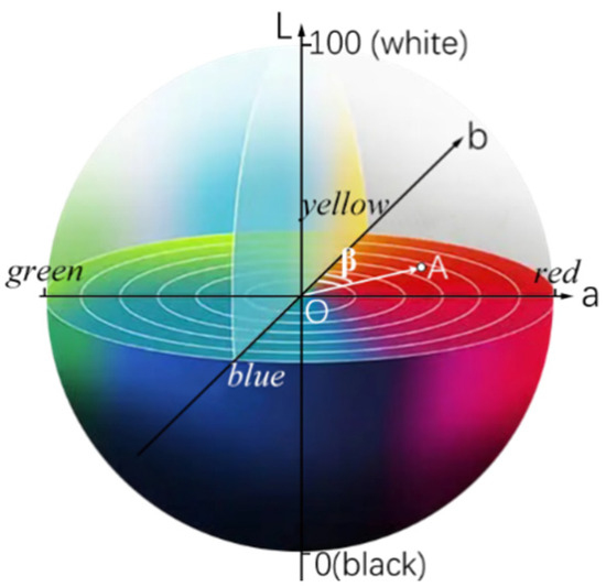
Figure 1.
CIE Lab color mode. The ‘L’ channel represents luminance. The ‘a’ channel represents the range from red to green and the ‘b’ channel represents the range from yellow to blue.
2.2. The Relationship between the Terrain Patterns and Normalized Topographic Relief
Sub-regional statistics are applied to quantify the relationship between the luminance values of the patterns and the normalized topographic relief. Detailed statistical analyses are conducted on the luminance value within different geomorphic units and different ranges of normalized relief values, thereby analyzing the spatial distribution of luminance and the correlation between the luminance and normalized topographic relief.
The correlation between the colors of the patterns and the change rate of normalized topographic relief is analyzed. Specifically, the color vector at each grid cell in the patterns is constructed with the ‘a’ and ‘b’ values in the Lab color space, and the angle between the color vector and the positive direction of the b-value axis is calculated using the following equation:
Each image is composed of three normalized topographic relief layers so that the values at the grid cells are respectively recorded as τr, τg, and τb. That is,
We regard red and blue grid cells of the patterned image as the typical research objects. The angle β at these cells falls within the ranges of 45 to 90 and 180 to 225. Subsequently, the angular difference between the red pixels and the positive direction of the b-value axis is calculated, and then, the angle between the blue pixels and the negative direction of the b-value axis is determined as well, denoted as Δβ. A scatter plot comparing Δβ and k is created to examine their correlation.
2.3. Flux and Curl of Topographic Field
In contrast to the electromagnetic field, NAW corresponds to a closed loop in the field while the normalized topographic relief τ(w) corresponds to the magnetic field. As the window size w changes, the variation of τ(w) within the window induces changes in the luminance and color of the terrain patterns (differentiation of color vectors). Therefore, the concept of ‘topographic field’ and formulas referring to Maxwell’s equations [15] are introduced. Within a specific observation range S, we measure the integral of τ(w) and its variation, denoting them as the topographic field flux and curl, respectively.
The integration of τ(w) within the observation range S is defined as the topographic flux φ, and thus, φ is expressed as below:
Here, a denotes the size of a given observation scale.
When φ changes, the curl of the topographic fields is defined as below:
Here, O denotes the topographic field.
2.4. Validation of Topographic Field Parameters for the Interpretation of Terrain Patterns
This section primarily focuses on validating the consistency of changes in topographic field flux and curl concerning scale variations in terrain patterns. Specifically, a region with diverse landforms is selected for validation, and the DEM data of this region are presented in Section 2.5.
The validation process involved several steps. First, using NAWs with incrementing sizes, a normalized relief sequence was constructed for the study area according to Equation (1). Different normalized relief layers were composed to create composite images, as illustrated in Section 2.1. One of the patterned images with distinct differentiation was selected for a case study. The NAW corresponding to the red band of this image was denoted as w1 while the NAW to the blue band was denoted as w2. Second, based on Equations (5) and (6), the flux and curl of the topographic field in the study area were calculated for w = w1 and w = w2. Third, with the NAW size ranging from w1 to w2, the average flux of the topographic observation field was calculated as = [φ(w1) + φ(w2)]/2. Subsequently, a scatter plot of and luminance of terrain patterns were drawn. Fourth, the vector V was defined from the origin (0, 0) to the endpoint (curl(w1), curl(w2)), and the angle βcurl between vector V and the positive Y-axis was calculated. The value of βcurl ranged from 0° to 360°. The spatial and quantitative distribution of βcurl were compared with the spatial distribution of the pattern color vector βcolor to verify their correspondence.
2.5. Data for Terrain Pattern Analysis and Validation
To simplify the analysis, an artificial digital elevation model was constructed and used as a source of sample data for analyzing the relationship between the terrain patterns and normalized topographic relief. The constructed DEM presented a basic landform structure with one independent hill and two adjacent hills. Patterns formed from simple terrain structures are conducive to effective analysis, mitigating the superposition of scale effects caused by the complex landforms or uncertainty introduced by neighboring terrains.
The artificial DEM was generated using the ‘peaks’ function (Equation (7)) in Matlab 2012a, representing a typical landform that conforms to the Gaussian distributions.
The positive values of the ‘peaks’ function were scaled by a factor of 1000 and the negative values were set to zero. The numerical values of the surface were recorded in a 60 × 60 matrix. The values of the DEM ranged from 0 to 850. Then, the matrix was exported to a raster file in GeoTiff format, with the length and width set to 6 km each (Figure 2a).

Figure 2.
Sample data. (a) Three-dimensional view of the data. (b) Contours with topographic feature lines on the DEM.
The study area for validation spans from the Tibet Plateau in the west to the Wuyi Mountains on the southeast coast of China (Figure 3), encompassing a diverse array of landforms to ensure variations in terrain scale features. The data of normalized topographic relief were produced using SRTM3 data with a 3 arc-second (~90 m) resolution. During data preprocessing, extra attention was paid to detection and elimination of noise, particularly high outliers, within the SRTM3 data. This involved the application of a combination of median filtering and Gaussian smoothing techniques to reduce noise while preserving the essential topographical features. The computational analysis of topographic relief properties and color pattern characterization was conducted using Python 3.9, employing its powerful libraries for geospatial data manipulation and image processing.

Figure 3.
The DEM of validation area covers the southeastern part of the Qinghai–Tibet Plateau, Hengduan Mts., Sichuan Basin, and the hilly regions in Fujian and Zhejiang Provinces, China, exhibiting diverse landforms.
3. Results
3.1. Terrain Patterns
Following the terrain-pattern composite method in Section 2.1, a new series of false-color images were generated using normalized topographic relief layers derived from the sample DEM. The patterns emerged prominently in the hilly areas in the sample DEM (Figure 4). Flat areas exhibit no discernable patterns while transitional terrains like ridges and foothills display subtle patterns. The landform features such as saddle and ridge lines were directly discernable in the patterns, in contrast to their subtle representation in the DEM. Sharp hills appeared brightest in the images while the gentle slopes exhibited less pronounced features, indicating differences in the scale response of different parts of the terrain.

Figure 4.
False-color images with different normalized topographic relief layers. (a) Composite image created by blending R5, R7, and R9, with ridge and saddle lines overlayed. (b) Composite image of R5, R9, and R13, with the contours overlayed as a reference of topography and the contours acting as a reference for the terrain’s morphology, corresponding to the pattern colors. (c) Composite image of R5, R11, and R17, with six points marked off for further analysis.
For further scale signature analysis, six sites with distinct pattern features were selected. Points V1 and V4, V2 and V5, and V3 were positioned at typical blue, green, and red cells of the image, respectively, while V6 was situated on flat terrain for comparison.
The color distinctions in the patterns were evident and consistent, but irrelevant to the steepness of the terrain. Altering the layers constituting an image resulted in variations in pattern detail while the overall spatial structures remained similar.
In the validation area, the terrain patterns at different scales also exhibited similarities, similar to the patterns in Figure 4. Geomorphic regions with different landforms presented distinct colors and textures (Figure 5).
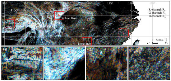
Figure 5.
Image showing terrain patterns of the actual land surface, created using R9, R19, and R29. (a) Stretching branch of Gangdise, fault-block mountains; (b) Qionglai Mts., fold mountains; (c) Karst landform area (southern part); and (d) southeast hills in China, granite hilly area.
The patterns exhibited significant distinctions across the regions. In mountainous areas surrounding the high-altitude Qinghai–Tibet Plateau with large topographic relief, the terrain patterns mainly appeared in a brighter blue, with distinct structural differences in fault-block mountains (Figure 5a) and folded ranges (Figure 5b). In karst landform areas featuring minor relief and low hills, the dominant patterns displayed an irregular dark red color (the lower half of Figure 5c). In the hilly terrain of the southeast, the patterns demonstrated a relatively balanced proportion of different colors, often exhibiting circular or granular textures (Figure 5d).
3.2. Luminance of the Terrain Patterns and the Normalized Topographic Relief
The sample data were divided into three sections for analysis: hilly grid cells, ridge line and saddle cells (Figure 4a), and flat terrain cells. The luminance of each part was quantified using a compressed boxplot. In general, the hilly areas exhibited significantly higher luminance than the flat terrain (Figure 6a), indicating that the luminance of terrain patterns could serve to distinguish between mountains and non-mountain areas. The average normalized topographic relief of the hilly section was 0.89, with an average luminance of 77.13. In comparison, the average normalized topographic relief of the flat surface was 0.11, with an average luminance of 33.04. Interestingly, ridge and saddle areas, often considered distinctive positions, exhibited a secondary level of luminance, with an average normalized topographic relief of 0.61 and an average luminance of 69.40.
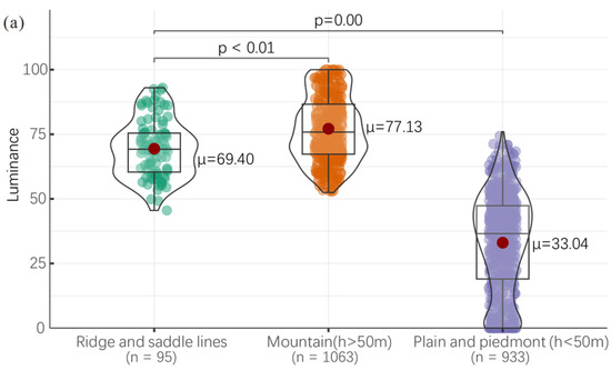
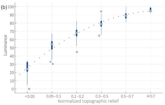
Figure 6.
Luminance of the patterns. The boxplots span the 25th to 75th percentiles. (a) Violin plots of the pattern luminance for three sections in the sample DEM, with the red dots in the plot indicating mean values. (b) Correlation between luminance and normalized topographic relief.
As the normalized topographic relief increased, the luminance followed a corresponding increase (Figure 6b).
3.3. Relationship between Color Differences and Change in Normalized Topographic Relief
The scale signature of normalized topographic relief was sampled using NAW sizes ranging from three to twenty-one grid cells with an increment step of two. Six observation sites, shown in Figure 4c, provided representative cases of varied trends. As shown in Figure 7, the curve’s monotonicity was not consistent across all points, but it stabilized when the window size exceeded 13 grid cells. For V1 and V4, curves kept increasing, corresponding to the blue hue of the patterns. V2 and V5 exhibited curves that initially increased and then decreased, with a green hue in the patterns. V3 showed the curve that continuously decreased when the size of the NAW was less than 17 grid cells, and the hue of the point was red. For V6, the value of the curve remained nil until the window size was large enough to include cells of the hilly area.

Figure 7.
Scale signature of the normalized topographic relief at observation sites.
Taking any three values on one curve, denoted by τ1, τ2, and τ3 in order, when τ3 > τ2∧τ2 > τ1, the pattern cell appeared blue; when τ1 > τ2∧τ2 > τ3, the pattern cell appeared red; when τ2 > τ1∧τ3 > τ2, the pattern cell appeared green. Generally, the colors at the observation sites aligned well with the scale signature of the normalized relief.
The color vectors (Equation (2)) were drawn to show the direction of the color vector at each grid cell (Figure 8a). The small dots in the figure represent the cells with luminance values of less than 30, corresponding to plain areas. The arrows’ directions are consistent with the color attributes.

Figure 8.
(a) Color vectors of the grid cell in Figure 4b. (b) Correlation between the change rate of the normalized relief and the rotation angle of the color vectors (only blue-hued grid cells selected). (c) Correlation between the change rate of the normalized relief and the rotation angle of the color vectors (only red-hued grid cells selected).
By plotting the k (Equation (3)) and Δβ (Equation (4)) of the color vectors in a scatter diagram, we found that the angle change in the color vector has an approximate linear relationship with the relief change ratio (Figure 8b,c). The change rate is positively correlated with the rotation angle of the color vector. Thus, it can be inferred that the change rate of the normalized relief caused the rotation of the color vector, leading to the color differences observed.
3.4. Comparison between the Terrain Patterns and the Flux and Curl of Topography Field
The patterned image of the validation areas was generated with R9, R19, and R29. Subsequently, calculations were performed using Equations (5) and (6) to derive the values of , curl(9), and curl(29), with S = 9 as the reference scale. Comparing the luminance of the patterns with , their spatial distribution characteristics were found consistent (Figure 9a,b). The quantity distribution also exhibited a linear correlation (Figure 9c). This suggests that within the same scale range, the average flux of the topographic field and the luminance of the patterns convey equivalent information.
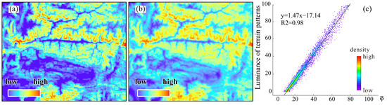
Figure 9.
Comparison between the luminance of the pattern (L) and the flux of the topographic field . (a) Luminance of the sample image. (b) Topographic flux in the sample area. (c) Scatter plot showing L and .
The angle βcurl was calculated based on curl(9) and curl(29); βcolor was based on the values ‘a’ and ‘b’ of the terrain-pattern colors (Figure 10(b-1–b-4)). The comparison of four local sample areas revealed spatial distribution similarities between βcurl and βcolor (Figure 10(a-1–a-4,b-1–b-4)), which were also reflected in numerical distributions (Figure 10(c-1–c-4,d-1–d-4)). For instance, in the Qionglai Mts., grid cells with βcurl ranging from 190° to 200° constituted the peak of the histogram. Overall, the variations in the curl of the topographic field could explain the color distribution characteristics in the map. Additionally, βcurl was calculated based on the integration of the regional integral, providing a better presentation of overall regional characteristics, which was a primary factor for the distinction between βcurl and βcolor.
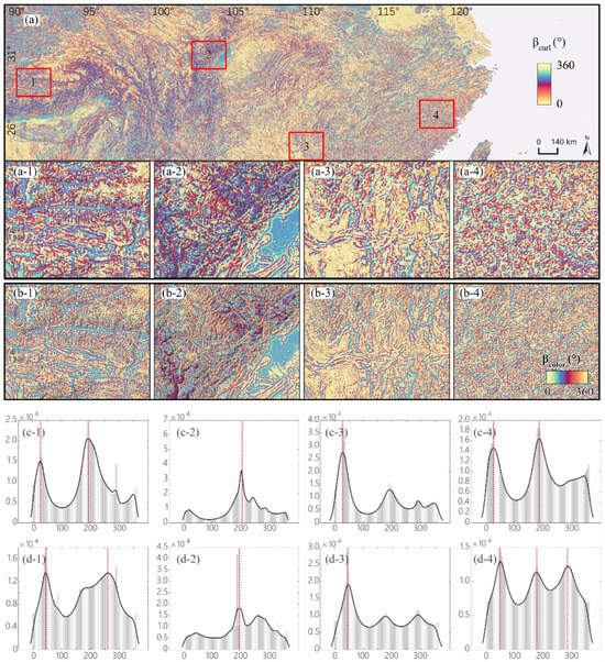
Figure 10.
Comparison between βcurl, the characteristic angle of the topographic field curl, and βcolor, the characteristic angle of the pattern color vector. (a,a-1–a-4) Overall distribution of βcolor in the study area and local magnifications in four geomorphic sample areas. (b-1–b-4) Distribution of βcolor in four geomorphic sample areas. (c-1–c-4) Histogram of βcurl, with the red dashed lines indicating the positions of the extreme values. (d-1–d-4) Histogram of βcolor, with the red dashed lines indicating the positions of the extreme values.
4. Discussion
We know that mapping landform is important as it can reflect physiographic regions, geological structures, and slope materials and processes [16,17], providing important reference value for understanding geomorphological evolution and guiding human activities such as agricultural production [18]. Since the 1950s, terrain analysis and mapping have been in a quantitative phase. Hammond was among the first to devise a numerical procedure to map terrain types using geometric criteria, primarily slope gradient, relative relief, and surface pattern or profile [19]. Subsequently, the numbers of parameters involved in terrain classification have continually increased. For instance, Iwahashi et al. used three taxonomic criteria—slope gradient, local convexity, and surface texture—for automated topography classification [20]. The common feature of such methods is that they are based on a geometric signature. However, many geometric measures, such as relative relief and the standard deviation of elevation, the hypsometric integral, and skewness of elevation, describe the same attribute of surface form and thus are redundant; for this reason, “new” geomorphometric parameters are rarely introduced [21]. To explore more pathways for terrain analysis, this paper has conducted a quantitative analysis from the perspective of “scale features” rather than “geometric signature” and provided a preliminary interpretation of the information contained within these scale characteristics.
Given the intricate nature of scale features, prior studies have often mapped differences in geomorphic features at various scales or employed the scale signatures of terrain attributes at ground sampling points to investigate topographic scale effects. While these approaches offer valuable insights, they have limitations. For example, a change in scale resulting in different geomorphon mapping results directly reflects the impacts of scale, but provides limited interpretation for scale effects. As for the scale signature method, the spatial representativeness of ground sampling points is limited, making it hard to reflect terrain scale features in contiguous space. As an extension of the scale signature method, an MTPCC image [7] serves to visualize the scale-variant topographic character of a landscape. However, it has predominantly been used for the visual interpretation of topographic position, rather than delving into the mechanisms responsible for the spatial differentiation of scale features or exploring its capacity to characterize topographic scale effects. This study introduced terrain patterns generated by blending normalized topographic relief images. Considered as valid terrain information for interpretation, the patterns offer an effective means to visualize the features of terrain scales. By sequentially analyzing terrain patterns with increasing NAWs, the study established a comprehensive interpretation grounded in the curl and flux properties of the topographic field. Within a given scale, this method allows for the quantitative analysis and visualization of changes in terrain attributes caused by scale effects.
The introduced topographic field flux and curl have potential applications in regional landform classification and automated geomorphic recognition. For instance, in previous studies, mountains were defined and delineated using a combination of elevation, topographic relief, and slope (sometimes, topographic relief is used alone) [22]. One major bottleneck of this method is the lack of consensus on the thresholds of these parameters for delineation [23]. This has led to significant discrepancies, with global mountain coverage estimates varying by up to 60% [24]. Building on the research of this paper, topographic field flux can be considered to discriminate discrepancies between mountainous and flat surfaces, thereby proposing more concise and objective indicators for mountain delineation. Taking the Qionglai Mts.–Chengdu Plain region (Figure 5b and Figure 11a) as an example, sub-area iii represents a plain, with its topographic field flux concentrated in a low-value range (mean μ = 0.31) compared to sub-areas i and ii (Figure 11b), serving as an effective basis for delineating mountains and non-mountain areas.
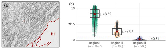
Figure 11.
Topographic field flux in different geomorphic areas. (a) Sub-area i is dominated by the Qionglai Mts., including parts of the Longmen Mts., with large undulating mountains and high mountains as the main features. Sub-area ii is dominated by small undulating low mountains. Sub-area iii is the Chengdu Plain. (b) Topographic field flux for the three sub-areas in the window size range of 9 to 29 pixels, with an observation baseline scale of 5 km.
Moreover, changes in curl in the same type of geomorphic region exhibit similarity. For instance, in the Gangdise Mts. branch sample area (Figure 10(a-1) and Figure 12a), the histogram and extreme point positions of βcurl in the distribution areas of the two fault-block mountains are similar (Figure 12b) while the histograms differ significantly in different geomorphic areas (Figure 10c-1–c-4). This provides a foundation for regional landform zoning and the automated recognition of special landforms based on differences in scale features.

Figure 12.
Changes in the topographic field curl of the Gangdise Mts. branch. (a) Spatial distribution of βcurl; both sub-areas i and ii are typical distribution of fault-block mountains. (b) The numerical distribution of βcurl in sub-areas i and ii, with the red dashed lines indicating the positions of the extreme values.
The complexity of landforms is due to the variety in the landscapes of landforms. In China alone, there are more than 2400 morphogenetic types of landforms [25], making the region a ‘mega-system’ comprising various subsystems of landforms. It is essential to comprehend this mega-system at various scales, particularly at larger scales such as the landscape and regional scales. However, current DEM-based topographic analyses often focus on local scales in a ‘nearsighted’ way [10], posing challenges in achieving a regional understanding of landform systems [26]. The scale-oriented terrain patterns proposed in this paper exhibit self-similarity at the landscape scale. However, the parameters of topographic field flux and curl merely describe the origin and scale effects of these patterns, failing to capture their self-organizing characteristics. Recognizing the close relationship between geomorphic landscapes and external dynamic conditions, as well as lithology, there is a need for further exploration into the self-organizing and self-similar features embedded within terrain patterns.
5. Conclusions
In conclusion, this study introduced a new approach to constructing and interpreting terrain patterns that was also useful to describe scale effects. The specific conclusions are as follows:
- Terrain patterns reflect topographic scale effects and can be constructed by blending layers of normalized topographic relief images. Simple simulated terrains constructed using mathematical surfaces and actual complex terrains can generate similar features in terrain patterns. Notably, terrain patterns exhibit self-similarity within the same landform area while distinct differences are observable between the patterns of different landforms.
- In the Lab color space, the luminance of the terrain patterns demonstrates a positive correlation with normalized topographic relief. Additionally, the angle of the color vector of these patterns exhibits a linear correlation with the rate of change in the topographic relief. The patterns represent a comprehensive manifestation of the quantity and scale signature changes in normalized topographic relief at three specified scales.
- Through validation on real land surfaces, terrain patterns can be further generalized to be interpreted as patterns formed by topographic field flux and curl with scale changes. When the observing scale changes from w1 to w2, the topographic scale effect is manifested as both specific terrain field curls and changes in topographic flux, which can be expressed as a binary tuple (, ).
This study contributed to the field of scale-oriented terrain analysis by introducing a quantitative method to depict and measure the subtle factors of terrain scale effects. By exploring the detailed information contained in these scale changes, this work extends beyond the traditional descriptive framework in geomorphology. This method enables terrain analysis to be conducted at a regional scale without considering the detailed features of the terrain.
An additional contribution of this research is the provision of reference indicators for identifying the self-similarity of terrain patterns in different geomorphic regions. These patterns, whether previously unrecognized or not fully explored, provide valuable insights into landform formation and evolution. They may offer a compelling framework to explain the interactions of geological history, climate forces, and human influence that shape the Earth’s topography. Utilizing these patterns enhances our understanding of geomorphic processes.
Overall, this study marked a useful exploration towards understanding and quantifying the complex characteristics of Earth’s terrain. Through its innovative methodology, it may enrich the theoretical foundation of geomorphology and provides practical tools for interpreting the intricate stories engraved on the planet’s surface.
Author Contributions
Conceptualization: Xi Nan, Ainong Li and Zhengwei He; methodology: Xi Nan, Ainong Li and Zhengwei He; software: Xi Nan and Jinhu Bian; validation: Xi Nan, Ainong Li, Zhengwei He and Jinhu Bian; formal analysis: Xi Nan; investigation: Xi Nan; data curation: Xi Nan; writing—original draft preparation: Xi Nan; writing—review and editing: Ainong Li, Zhengwei He and Jinhu Bian; visualization: Xi Nan; supervision, Ainong Li and Zhengwei He. All authors have read and agreed to the published version of the manuscript.
Funding
This research was jointly funded by the National Key Research and Development Program of China [2020YFA0608702], the Strategic Priority Research Program of the Chinese Academy of Sciences [XDA19030303], the National Natural Science Foundation of China [42171382; 41971226; 41871357], and the Science and Technology Research Program of the Institute of Mountain Hazards and Environment, Chinese Academy of Sciences (IMHE-CXTD-03).
Data Availability Statement
Data will be made available on request.
Acknowledgments
We sincerely thank Tina Song and Amin Naboureh for proofreading and polishing this paper.
Conflicts of Interest
The authors declare no conflicts of interest.
Abbreviations
| Abbreviation | Explanation |
| CIE | International Commission on illumination |
| DEM | digital elevation model |
| DEV | deviation from mean elevation |
| Lab | Lightness, a-b chromaticity (a color space used in digital imaging) |
| MTPCC | multi-scale topographic position color composite image |
| Mts. | mountains |
| NAW | neighborhood analysis window |
| SRTM3 | NASA Shuttle Radar Topography Mission data with a 3 arc-second resolution |
References
- Drăguţ, L.; Eisank, C. Object representations at multiple scales from digital elevation models. Geomorphology 2011, 129, 183–189. [Google Scholar] [CrossRef]
- Li, Z. Multi-scale digital terrain modelling and analysis. In Advances in Digital Terrain Analysis; Zhou, Q., Lees, B., Tang, G., Eds.; Springer: Berlin, Germany, 2008; pp. 59–83. [Google Scholar]
- Gallant, J.C.; Wilson, J.P. Primary topographic attributes. In Terrain Analysis: Principles and Applications; Wilson, J.P., Gallant, J.C., Eds.; John Wiley & Sons Inc.: New York, NY, USA, 2000; pp. 51–85. [Google Scholar]
- Deng, Y. New trends in digital terrain analysis: Landform definition, representation, and classification. Prog. Phys. Geogr. 2007, 31, 405–419. [Google Scholar] [CrossRef]
- Lindsay, J.; Newman, D. Hyper-scale analysis of surface roughness. PeerJ Prepr. 2018, 6, e27110v1. [Google Scholar] [CrossRef][Green Version]
- Tate, N.J.; Wood, J. Fractals and scale dependencies in topography. In Modelling Scale in Geographical Information Science; Tate, N.J., Atkinson, P.M., Eds.; John Wiley and Sons: Chichester, UK, 2001; pp. 35–51. [Google Scholar]
- Lindsay, J.; Cockburn, J.; Russell, H. An integral image approach to performing multi-scale topographic position analysis. Geomorphology 2015, 245, 51–61. [Google Scholar] [CrossRef]
- Jasiewicz, J.; Stepinski, T.F. Geomorphons—A pattern recognition approach to classification and mapping of landforms. Geomorphology 2013, 182, 147–156. [Google Scholar] [CrossRef]
- Zhang, W.; Li, A. Study on the optimal scale for calculating the relief amplitude in China based on DEM. Geogr. Geo-Inf. Sci. 2012, 28, 8–12. (In Chinese) [Google Scholar]
- Tang, G.; Na, J.; Cheng, W. Progress of Digital Terrain Analysis on Regional Geomorphology in China. Acta Geod. Cartogr. Sin. 2017, 10, 1570–1591. (In Chinese) [Google Scholar]
- Nan, X.; Li, A.; Chen, Y.; Deng, W. Design and compilation of digital mountain map of China (1:6,700,000) in vertical layout. Remote Sens. Technol. Appl. 2016, 31, 451–458. (In Chinese) [Google Scholar]
- Tagil, S.; Jenness, J. GIS-based automated landform classification and topographic, landcover and geologic attributes of landforms around the Yazoren Polje, Turkey. J. Appl. Sci. 2008, 8, 910–921. [Google Scholar] [CrossRef]
- Nan, X.; Li, A.; Jing, J. Calculation and verification of topography adaptive slide windows for the relief amplitude solution in mountain areas of China. Geogr. Geo-Inf. Sci. 2017, 33, 34–39. (In Chinese) [Google Scholar]
- De Reu, J.; Bourgeois, J.; Bats, M.; Zwetvaegher, A.; Gelorini, V.; Smedt, P.D.; Chu, W.; Antrop, M.; DeMaeyer, P.; Finke, P. Application of the topographic position index to heterogeneous landscapes. Geomorphology 2013, 186, 39–49. [Google Scholar] [CrossRef]
- Wang, Z. On the first principle theory of nanogenerators from Maxwell’s equations. Nano Energy 2020, 68, 104272. [Google Scholar] [CrossRef]
- Cheng, W.; Wang, N.; Zhao, M.; Zhao, S. Relative tectonics and debris flow hazards in the Beijing mountain area from DEM-derived geomorphic indices and drainage analysis. Geomorphology 2016, 257, 134–142. [Google Scholar] [CrossRef]
- Hengl, T.; Rossiter, D. Supervised landform classification to enhance and replace photo-interpretation in semi-detailed soil survey. Soil Sci. Soc. Am. J. 2003, 67, 1810–1822. [Google Scholar] [CrossRef]
- Valjarević, A.; Popovici, C.; Štilić, A. Cloudiness and water from cloud seeding in connection with plants distribution in the Republic of Moldova. Appl. Water Sci. 2022, 12, 262. [Google Scholar] [CrossRef]
- Hammond, H. Analysis of properties in land form geography: An application to broad-scale landform mapping. Ann. Assoc. Am. Geogr. 1964, 54, 11–19. [Google Scholar] [CrossRef]
- Iwahashi, J.; Pike, J. Automated classifications of topography from dems by an unsupervised nested-means algorithm and a three-part geometric signature. Geomorphology 2007, 86, 409–440. [Google Scholar] [CrossRef]
- Pike, J. “Topographic fragments” of geomorphometry, GIS, and DEMs. In DEMS and Geomorphology, Geographic Information Systems Asssociation (Japan) Special Publication, Proceedings of the 5th International Conference on Geomorphology; Chuo University: Tokyo, Japan, 2001; pp. 34–35. [Google Scholar]
- Karagulle, D.; Frye, C.; Sayre, R.; Breyer, S.; Aniello, P.; Vaughan, R.; Wright, D. Modeling global Hammond landform regions from 250-m elevation data. Trans. GIS 2017, 5, 1040–1060. [Google Scholar] [CrossRef]
- Snethlage, M.A.; Geschke, J.; Ranipeta, A.; Jetz, W.; Yoccoz, N.; Körner, C.; Spehn, E.M.; Fischer, M.; Urbach, D. A hierarchical inventory of the world’s mountains for global comparative mountain science. Sci. Data 2022, 1, 149. [Google Scholar] [CrossRef]
- Körner, C.; Jetz, W.; Jens, P.; Payne, D.; Rudmann-Maurer, K.; Spehn, E.M. A global inventory of mountains for bio-geographical applications. Alp. Bot. 2017, 127, 1–15. [Google Scholar] [CrossRef]
- Zhou, C.; Cheng, W.; Qian, J. Research on the classification system of digital land geomorphology of 1:1,000,000 in China. J. Geo-Inf. Sci. 2009, 6, 707–724. (In Chinese) [Google Scholar]
- Xiong, L.; Li, S.; Tang, G.; Strobl, J. Geomorphometry and terrain analysis: Data, methods, platforms and applications. Earth-Sci. Rev. 2022, 233, 104191. [Google Scholar] [CrossRef]


Disclaimer/Publisher’s Note: The statements, opinions and data contained in all publications are solely those of the individual author(s) and contributor(s) and not of MDPI and/or the editor(s). MDPI and/or the editor(s) disclaim responsibility for any injury to people or property resulting from any ideas, methods, instructions or products referred to in the content. |
© 2024 by the authors. Licensee MDPI, Basel, Switzerland. This article is an open access article distributed under the terms and conditions of the Creative Commons Attribution (CC BY) license (https://creativecommons.org/licenses/by/4.0/).