Article

Optimizing Station Placement for Free-Floating Electric Vehicle Sharing Systems: Leveraging Predicted User Spatial Distribution from Points of Interest

School of Transportation, Southeast University, Nanjing 211189, China
*
Author to whom correspondence should be addressed.
ISPRS Int. J. Geo-Inf. 2024, 13(7), 233; https://doi.org/10.3390/ijgi13070233
Submission received: 25 March 2024 / Revised: 18 June 2024 / Accepted: 25 June 2024 / Published: 1 July 2024

Abstract

:
Rapid growth rate indicates that the free-floating electric vehicle sharing (FFEVS) system leads to a new carsharing idea. Like other carsharing systems, the FFEVS system faces significant regional demand fluctuations. In such a situation, the rental stations and charging stations should be constructed in high-demand areas to reduce the scheduling costs. However, the planning of the FFEVS system includes a series of aspects of rental stations and charging stations, such as the location, size, and number, which interact with each other. In this paper, we first provide a method for forecasting the demand for car sharing based on the land characteristics of Beijing FFEVS station catchment areas. Then, the multi-objective MILP model for planning FFEVS systems is developed, which considers the requirements of vehicle relocation and electric vehicle charging. Afterward, the capabilities of the proposed models are demonstrated by the real data obtained from Beijing, China. Finally, the sensitivity analysis of the model is made based on varying demand and subsidy levels. From the results, the proposed model can provide decision-makers with useful insights about the planning of FFEVS systems, which bring great benefits to formulating more rational policies.

1. Introduction

Federal Highway Administration studies showed that the average travel distance of a private vehicle is around 40 km per day, which is approximately 90 min [1]. The rest time of this vehicle is idle and used to find a parking position. The International Energy Agency indicated that vehicles’ emissions account for around one-third of the world’s carbon emissions, which is predicted to exceed 50% by 2030 [2]. In such a background, electric vehicle sharing (EVS) was proposed, which attracted considerable attention around the world due to its abilities to improve mobility and sustainability [3]. Recently, some studies showed that such a system was beneficial to solving congestion and environmental pollution problems [4,5,6,7,8,9]. In addition, providing economically disadvantaged groups with an affordable price is another benefit [10,11,12].
Based on the locations where the rented cars are returned, the EVS systems can be divided into two different types: flexible “free-floating electric vehicle sharing (FFEVS)” and more restricted “two-way electric vehicle sharing (TWEVS)”, respectively. The FFEVS system means that users can pick up or drop off vehicles in any parking spot within the borders of an area; however, the TWEVS system requires users to pick up and drop off the rented cars in a fixed parking spot.
The attractiveness of EVS systems is generally determined by the service level and the cost. Specifically, the service level is influenced by the accessibility of vehicle stations. It mainly includes two aspects, for one thing, the distance between the user’s origin and destination from pick-up and drop-off vehicle stations, respectively, and another one is the availability of vehicles at stations. Regarding the cost, the main influence factors include the number and size of stations, fleet size, and availability of vehicles [13].
Ensuring vehicle availability and station accessibility is a prominent problem when vehicles can be rented and used on FFEVS systems. For example, the free-floating operation of the vehicles is coupled with the imbalanced demand of vehicles at the origin of the trip (pick-up station) and at the destination (drop-off station), which can cause vehicles to accumulate at some stations where they are not needed. Thus, precisely predicting the user demand of the rental station and rationally planning the location of the rental station are the keys to improving operational revenue [14].
Unlike traditional fuel vehicle sharing systems, the flexibility of the FFEVS system is limited by the charging problem. In general, the rental stations of FFEVS are usually located in public and commercial parking lots. As the electric vehicles are still in the initial stage of development, the charging facilities are not yet fully equipped, and only a few parking lots have installed the charging piles. In such a situation, the vehicles need to go to a nearby FFEVS rental station with charging facilities or a rental charging station. In addition, the charging time will affect the availability of the vehicle, and the accessibility of the charging station will affect the charging and scheduling costs of the vehicle. It is important to consider the configuration of the charging station, which can improve vehicle availability and reduce operating costs [15]. Thus, efficient strategic planning should be implemented, such as introducing models into one-way car-sharing systems to optimize the number and location of the service stations, the fleet size, and the dynamic allocation of vehicles to stations. And those models can help decision-makers achieve a balance between the level of service and the total cost (including vehicle relocation costs).
Therefore, scientifically determining the use demand of shared cars and developing effective station (rental stations and charging stations) layout optimization methods based on this user demand is the core content of ensuring the orderly development of shared cars and also the key to exerting the advantages of shared cars in alleviating traffic congestion, reducing energy consumption, and reducing environmental pollution.
However, the literature currently lacks a model that can jointly optimize rental station locations, the size of the EV fleet, and charging station locations, while considering the dynamics of vehicle relocation and balancing for a system with reservations. Existing models [16] either look at station locations without consideration of vehicle relocation decisions or assume that only the demand in the catchment area of opened stations needs to be served. In the case where vehicle relocation is modeled, the relocation of the vehicles and the associated costs are considered only at the end of the operating period (usually a day), which will influence the fleet size [17]. Studies related to EVS station location planning are summarized in Table 1.
The objective of this paper is threefold: (i) Develop and validate a series of carsharing demand forecast models for determining the rental station locations and fleet size of FFEVS; (ii) develop a mathematical model for determining the optimum fleet size, and the number and location of the required stations of FFEVS with consideration of dynamic vehicle repositioning (relocation); and (iii) apply the proposed model to plan and operate a FFEVS system in the city of Beijing, China.

2. Methodology

Figure 1 shows the framework of our methodology, which encompasses three core components: (i) Estimating the radiation scope of one station by surveying users’ maximum acceptable travel time; (ii) forecasting the demand distribution of carsharing with the travel purposes of the residents and the land use indicators; and (iii) constructing an integrated station optimization model based on the predicted carsharing demand to maximize operators’ profits.

2.1. Station Radiation Scope

The influence scope of an EVS station refers to the maximum radiation range of the station. The radiation scope can be formed by taking the station as the center and the acceptable distance as the radius; the acceptable radius is the distance from the starting point to the rental station.
To investigate the maximum acceptable distance and mode of transfer when people choose to use EVS, a paper questionnaire and an online electronic survey are applied in this research. The survey collected a total of 892 valid questionnaires, and the results showed that the proportion of people walking ranked first, which was around 86%. Due to the figures for other transfer methods being less than 10%, those ways were not analyzed in this research. The statistical results of the questionnaire showed that the average walking speed is 5 km/h, the probability density is the normal distribution, and the distance at the cumulative probability of 85% is the walking distance. In addition, the maximum acceptable distance for users is 921.65 m in this paper.
In general, the actual transfer distance for passengers is greater than the straight distance from the starting point of the trip to the railway station. The transfer distance can be ensured after correcting the road network’s characteristics [4]. In this research, the road network is mostly square in Beijing. Thus, the actual passenger transfer distance can be expressed as [30]
L = L 1 + L 2 = R ( sin α + cos α ) = 2 sin ( α + π / 4 )
where L is the actual transfer distance; L 1 and L 2 are the length of the side of the road; R is the straight distance from a point to the electric vehicle sharing station. Calculated by Equation (1), the actual passenger transfer distance of Beijing is 651.71 m.

2.2. Demand Prediction

The demand forecast model consists of three parts: data investigation, land use index, and the construction and verification of the demand model. Based on the residents’ main purpose of travel, the characteristics of various land use types are refined, and land use indicators and models are established to determine the demand distribution of electric vehicle sharing.

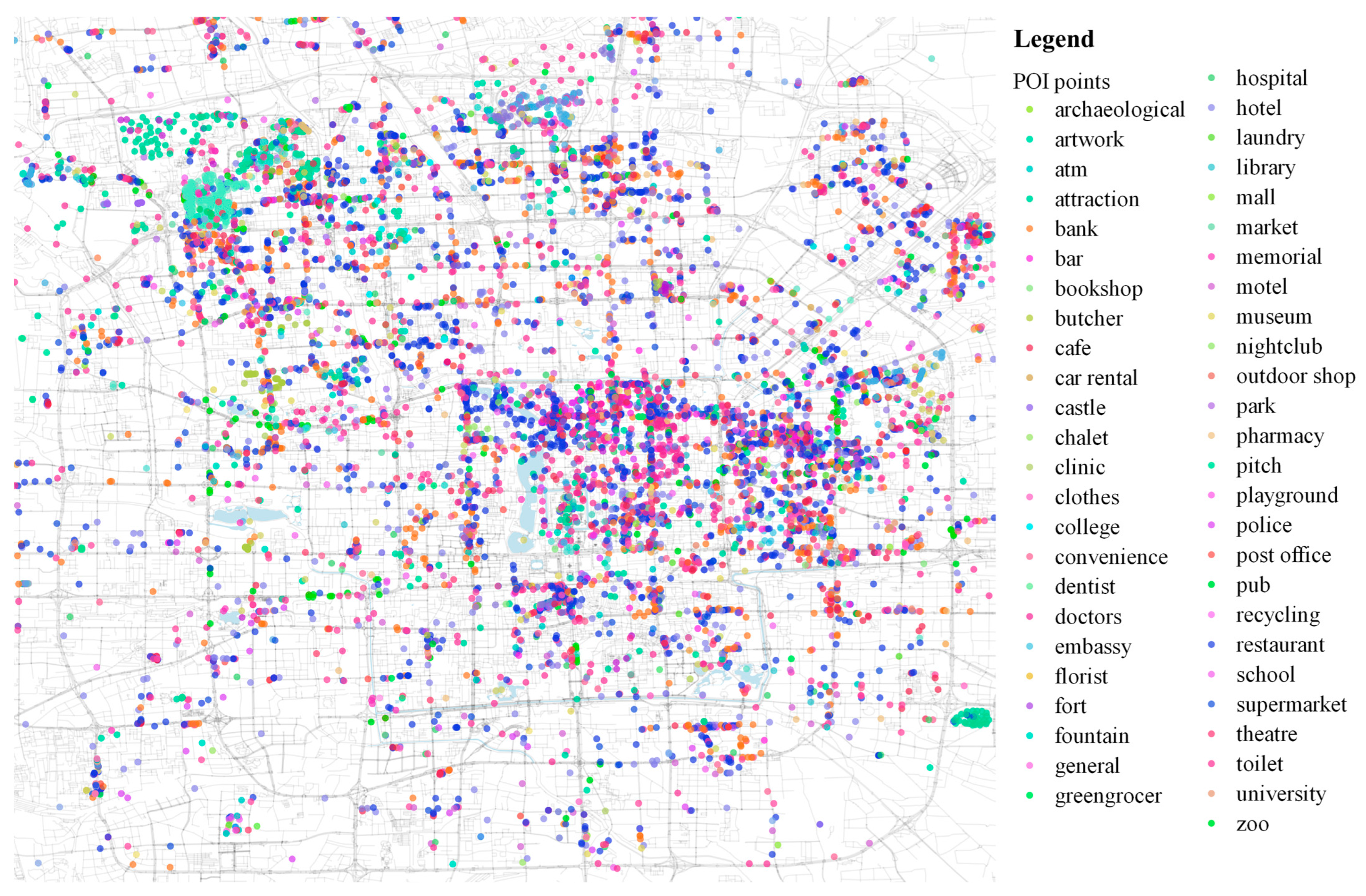
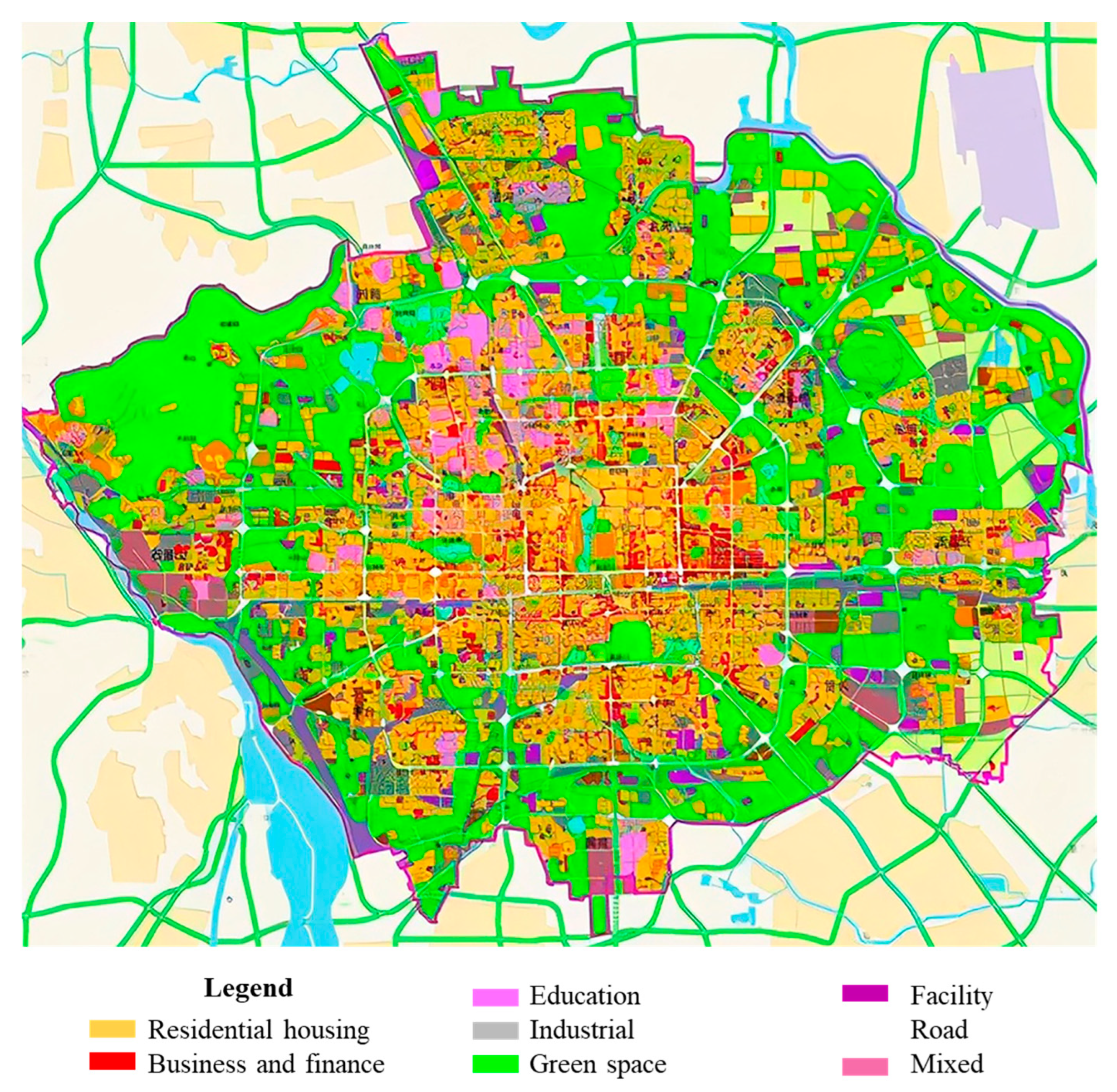
2.2.1. Data Resources

Operational data for an EVS company in Beijing was collected. The data mainly include vehicle GPS positioning data and order data. In this research, the total number of data points is 169,926 (year: 2020–2021), and the form of the data is shown in Table 2.
Firstly, the study investigated approximately 190,000 POIs within the Six Miles area of Beijing. Then the POIs are divided into six parts (education, leisure, residence, work, shopping, and other five categories) based on the main purpose of Beijing residents’ travel [31]. After that, the POIs are built according to the type of different databases with the help of GIS (Geographic Information System). Finally, using the influence radius of electric vehicle sharing stations as a radius buffer, we can obtain the number of various POIs within the scope of the station, as shown in Figure 2.

2.2.2. Index Selection and Construction

As we know, the building area is the main control index in the process of planning, which can significantly influence the population, social economy, and other indicators. Therefore, in this paper, a refinement analysis of the station was conducted by using the building area of interest within the scope of the attraction of the orbital station. In addition, this study uses the “total building area” and “land use different index” to represent the density and degree of land use, respectively. The results are regarded as the basis for constructing a demand model for electric vehicle sharing stations.
Based on the refined database of the land in Beijing, the number of POIs within the influence scope of each station is acquired through ArcGIS. Using the average building area of various interest points obtained from the survey [31], the various POIs within the area are converted into building areas, which include education building area A e i , work building area A w i , residential building area A r i , commercial building area A s i , leisure building area A l i . The total number of POIs for each station is termed as A t i .
From the travel mechanism of electric vehicle sharing, regardless of whether the travelers’ purpose is working, going to school, or shopping, the land use for starting and ending is different [32]. For example, when you travel for work, the starting point is often residential land, the end point is work land and the return journey is the opposite. There are fewer trips from work land to work land, or from residential land to residential land [33]. Extending this reason to the accumulative level, it can be considered that the difference in land use within the two attraction ranges is the driving force for traveling [34]. In other words, if there are fewer differences in land use between two different attractions, the attraction between those two places is less attractive. Conversely, the attraction is greater [35]. Based on the analysis, the land use disparity index between the different attractions can be expressed as
L i j = ( A e i A e j ) 2 + ( A w i A w j ) 2 + ( A r i A r j ) 2 + ( A s i A s j ) 2 + ( A l i A l j ) 2
In addition to land use factors, other alternative transportation modes are also playing an indispensable role in electric vehicle sharing travel. Considering that bicycles take up a small proportion of long-distance travel, the alternative transport modes mainly consider buses and private cars. The number of bus lines in the pedestrian zone and the number of parking are used to evaluate the impact of traffic demand factors on electric vehicle sharing stations. The number of bus lines and the number of parking spaces are counted by the number of corresponding POIs within the attraction range of the station.
Population is an important indicator of the intensity of land use. We obtain the total population ( P o i ) by adding the number of people in all POIs within the scope of the station. Apart from population, other social-economic data, such as the number of employees, can also explain the capacity of each zone to attract users more than other zones. They can be added to the EVS demand forecast model if other types of social-economic data are available.

2.2.3. Model Construction

Total traffic generation ( P i ), one-way traffic generation ( P s i , the rental station is different from the returning station), the round-trip traffic generation ( P r i , the rental station is the same as the returning station) and the total traffic attraction ( A i ) is selected as the dependent variable, respectively. The total building area ( A t i ), the number of bus lines ( B i ), the number of parking ( P a i ), and the population ( P o i ) within the influence scope of stations are the independent variables. The fitting results of the forecast models of total traffic demand are as follows:
P i = 0.750 A t i 0.028 P a i 0.196 B i + 0.251 P o i + ε
P s i = 0.688 A t i 0.022 P a i 0.154 B i + 0.352 P o i + ε
P r i = 0.743 A t i 0.030 P a i 0.209 B i + 0.180 P o i + ε
A i = 0.590 A t i 0.460 P a i 0.222 B i + 0.325 P o i + ε
Assume the number of orders ( R i j ) between stations i and station j as the dependent variable. The land use difference index ( L i j ), the total building area ( A t i ), the number of bus lines ( B i ), the number of parking ( P a i ), and the population ( P o i ) within the influence scope of stations are used to forecast R i j . The fitting result of the forecast model of traffic demand is given as follows:
R i j = 0.503 L i j 0.213 P a i 0.091 B i + 0.238 P o i + 0.861 A i + ε
As shown in Table 3, the fitness indexes ( R 2 ) of all models are greater than 0.7, indicating that the combination of independent variables selected by the model has a strong ability to interpret the dependent variables. In particular, Sig.s of L i j and A t i are less than 0.05, which confirms that land characteristic indexes have a significant correlation with the carsharing demand. We also observe that the Sig.s of some variables are far greater than 0.05, which should be excluded from the developed model. In practice, only variables with Sig.s less than 0.15 are added in the demand forecast models.

2.2.4. Model Test

In order to verify the accuracy of the model, select 20% of the small sample stations outside the 80% large sample of the calibration model to evaluate the predicted value. The predicted error E can be calculated by comparing the difference between the predicted value and the actual value:
E = ( R R ) / R
Table 4 reports the predicted errors of all stations in the testing dataset. The results showed that the 93.3% verification error is less than 20% and the 73.3% verification error is less than 15%. It is suggested that the models have good fitting effects and can provide a theoretical basis for the next section.

2.3. Station Optimization Function and Content

2.3.1. Problem Description

In this section, we address the problem of the electric vehicle-sharing system design. Locations of EVS rental stations and charging stations, the required EV fleet (the number of operational EVs), and the EV relocation activities (on a regular operation day) are chosen as decision variables. The main aims are to integrate several decisions under the same model and address the key operational issues that may emerge in practice. To this end, we divide the problem for the whole operation day into several steps, which were created within a MILP formulation. The general model framework computes several days of operation, maintaining the dimensioning data from previous iterations, re-computing the hour-operation MILP model, and updating the system design, until the configuration reaches a net revenue equilibrium, producing a stable and “optimal” system configuration.
The evaluation of the system’s net revenue results from the fares paid by users, which may cover the system costs that result from three main components: the construction of the EV rental and charging stations, the acquisition of the EV fleet, and the relocation operations of the EVs.
The following section presents the mathematical modeling of the hourly optimization model, which is further refined into sub-operation periods compatible with regular EV trips’ travel times.

2.3.2. Mathematical Formulation

The model presents the following formulation:
(1) Parameters
NotionsDescriptions
Sets
N = ( 1 , , i , , N ) set of all candidate stations for the location of rental stations, where N is the total number of rental stations;
Q = ( 1 , , q , , Q ) set of all candidate stations for the location of charging stations, where Q is the total number of charging stations;
R = ( 1 , , r , , R ) set of all candidate stations for the location of rental stations with charging function, where R is the total number of rental stations with charging function;
D = ( 1 , , d , , D ) set of demand from rental stations i to j at time step t;
V = ( 1 , , v , , V ) set of candidate trips during one day of operation;
K = ( 1 , , k , , K ) set of persons that perform trips v V ;
M = ( 1 , , m , , M ) set of relocation trips in one day;
T 1 = ( 1 , , t 1 , , T 1 ) set of operational time steps in one day;
T 2 = ( 1 , , t 2 , , T 2 ) set of relocation time steps in one day.
Decision variables
X v i j binary variable that defines if the trip v V uses the rental station i N and j N ;
Y m i q binary variable that defines if the charging trip m M uses the station i N and q Q ;
Z m q j binary variable that defines if the relocation trip m M uses the charging station q Q and rental station j N ;
U m i j binary variable that defines if the relocation trip m M uses the rental station i N and j N ;
S i t 1 integer variable that identifies the balance of EVs in rental station i N at time step t 1 T 1 ;
Y q   integer   variable   that   identifies   the   charging   capacity   of   charging   station   q Q ;
Z i integer variable that identifies the capacity of rental station i N ;
F integer variable that identifies the total EV fleet;
I i t 2 integer variable that identifies the number of EVs in rental station i N at time step t 2 T 2 ;
M i   integer   variable   that   identifies   the   number   of   EVs   that   need   to   be   relocated   in   rental   station   i N ;
R e i   integer   variable   that   identifies   the   number   of   EVs   that   need   to   be   recharged   in   rental   station   i N ;
M i j integer variable that identifies the number of EVs relocated from rental station i N to j N ;
R e i j   integer   variable   that   identifies   the   number   of   EVs   that   need   to   be   recharged   in   station   j є N   relocated   from   rental   station   i N ;
H k binary variable that defines if the person k K performs a trip.
Data
T i j   matrix   that   represent   the   travel   time   estimates   to   travel   from   rental   station   i N   to   j N with an EV;
D i j   the   matrix   that   represents   the   travel   distance   estimates   to   travel   from   rental   station   i N   to   j N with an EV;
U t 2   binary   variable   that   identifies   if   the   user   k K   already   used   the   system   in   a   step   t 2 T 2 ;
Z i t 2   integer   variable   that   identifies   the   capacity   of   rental   station   i N   obtained   in   a   step   t 2 T 2 ;
F t 2   integer   variable   that   identifies   the   total   EV   fleet   obtained   in   a   step   t 2 T 2 ;
B i t 2   integer   variable   that   identifies   the   number   of   EVs   that   did   not   arrive   at   the   rental   station   in   the   previous   step   t 2 .
Constants
Z m a x maximum capacity of rental stations;
Z m i n minimum capacity of rental stations;
P t fare rate of an EV per minute at step t 1 T 1 ;
P d fare rate of an EV per kilometer at step t 1 T 1 ;
C s space cost in station i N for one EV per time at step t 1 T 1 ;
C t docking cost of an electric vehicle per minute in rental station i N at step t 1 T 1 ;
C d docking cost of an EV per minute in charging station i N at step t 1 T 1 ;
R c   Relocation   cos t   of   moving   a   vehicle   from   rental   station   i   to   j   at   step   t 1 T 1 ;
V c fixed daily cost of each EV;
F m a x maximum number of EVs in the system;
t s total time traveled by all EVs;
S s electric vehicle hourly driving subsidy;
d N the normal trip distance of an EV with a fully charged state;
t N the normal charging time of an EV.
(2) Model construction
With above notations, the objective function is described by the following expression.
Revenue:
P t v   є   V i   є   N j   є   N X v i j D v T i j + P d v   є   V i   є   N j   є   N X v i j D v D i j + t s S s
Fleet cost:
V c F t
Depot cost:
C s q   є   N Y q + C t i   є   N Z i
Relocation cost:
R c ( v   є   V i   є   N j   є   N X v i j + m   є   M i   є   N k   є   Q Y m i k + m   є   M k   є   Q j   є   N Z m k j )
Charging cost:
C t t N ( v   є   V i   є   N j   є   N X v i j d i j d N + m   є   M i   є   N k   є   Q Y m i k d i k d N + m   є   M k   є   Q j   є   N Z m k j d k j d N + m   є   M i   є   N j   є   N U m i j d i j d N )
Net revenue:
N e t   r e v e n u e = R e v e n u e F l e e t   c o s t D e p o t   c o s t R e l o c a t i o n   c o s t C h a r g i n g   c o s t
The model is a mixed integer linear programming model with maximizing operator’s profit as the objective function. The main benefits and costs of vehicle operation are shared by all parts of the objective function, including revenue, vehicle costs, parking costs, scheduling costs, and charging costs. Among them, the content of “Revenue” mainly includes two major aspects: (1) The usage charges for renting the car; (2) the government’s subsidies t s S s to encourage the development of shared electric vehicles. The acquisition method of usage charges is the “time and mileage comprehensive charging method”, which is the most widely used and most acceptable to users at present. That is, the usage time v   є   V i   є   N j   є   N X v i j D v T i j and the driving mileage v   є   V i   є   N j   є   N X v i j D v D i j are, respectively, at their own unit price, and the final sum is added. The “Vehicle cost” is the daily loss value V c F t of the vehicle after purchase and is related to the purchase price and the sale price after a certain period. The “Depot cost” refers to the parking fee for the rental and parking of vehicles at stations, which usually includes two ways: parking in a specific area charged according to the leased area C s q   є   N Y q or parking space charged according to the number of parking spaces C t i   є   N Z i . The “Relocation cost” refers to the cost incurred by relocating a vehicle from spare stations to other stations with a shortage of vehicles and a demand for useful vehicles.
Vehicle relocation usually includes two ways: (1) For vehicles v   є   V i   є   N j   є   N X v i j with sufficient electricity, the original parking station directly relocates the vehicles to the rental station, which lacks the vehicles; (2) for vehicles with insufficient electricity, the original parking station first dispatches the vehicles m   є   M i   є   N k   є   Q Y m i k to the charging station for charging, and then the charging station relocates the vehicles m   є   M k   є   Q j   є   N Z m k j to the rental station, which lacks the vehicles. The “Charging cost” refers to the cost of electricity used to charge a used vehicle. According to the purpose of the vehicle’s power consumption, vehicle charging usually includes two ways: (1) For rental stations with a charging function, the staff charges at the rental stations, and the charging amount v   є   V i   є   N j   є   N X v i j d i j d N is the user’s power consumption; (2) for rental stations without a charging function, the staff will drive the vehicle to the charging station to complete charging and then relocate the vehicle to the rental station. The charging cost includes three parts: the power consumption of users ( m   є   M i   є   N j   є   N U m i j d i j d N ), the power consumption of staff driving vehicles to charging stations ( m   є   M i   є   N k   є   Q Y m i k d i k d N ), and the power consumption of staff relocating vehicles to rental stations ( m   є   M k   є   Q j   є   N Z m k j d k j d N ).
This solution space is subject to the following constraints:
v   є   V i   є   N j   є   N X v i j 1   i , j N , v V
m   є   M i   є   N j   є   N U m i j 1   i , j N , m M
m   є   M i   є   N q   є   Q Y m i q 1   i N , m M , q Q
m   є   M q   є   Q j   є   N Z m q j 1   j N , m M , q Q
Constraints (15)–(18) ensure that each trip is assigned only to one pair of origin-destination depots.
I i t 2 + S i t 1 Z i   i N , t 1 T 1 , t 2 T 2
Constraint (19) warrants that the instantaneous fleet available at depot i     N does not exceed the depot capacity.
I i t 2 + S i t 1 0   i N , t 1 T 1 , t 2 T 2
Constraint (20) ensures that the total number of electric vehicles docked at the depot or moving has to remain constant for the entire step t 2 T 2 .
F F m a x
Constraint (21) guarantees that the estimated fleet is smaller than a maximum threshold.
Z i Z m i n Y i   i N
Constraint (22) ensures that the capacity of a depot is greater than a minimum threshold.
R i j I i   i , j N
R i j Z j B j   i , j N
Constraints (23) and (24) set an upper bound to relocation from and to every station, respectively. This upper bound equals the number of operating parking spaces in all open stations.
M i r I i   i N , r R
M i r Z r B r   i N , r R
M i q I i   i N , q Q
M i q Z q B q   i N , q Q
Constraints (25)–(28) set an upper bound to relocation from and to every station, respectively. This upper bound equals the number of operating parking spaces in all open charging stations.
Y i Z i Z m a x     i N
Constraint (29) warrants that a depot is only considered when it presents capacity.
B i t 2 + v   є   V j   є   N X v i j D v +   r є   R M i r +   q є   Q M i q = I i t 2   i N , r R , q Q , t 2 T 2
Constraint (30) ensures that the sum of the number of vehicles leaving the station and the number of remaining vehicles matches the total number of vehicles on the station.
i     N I i t 2 = F     t 2 T 2
Constraint (31) guarantees that the fleet of time step t 2 T 2 is distributed in its initial time step t 1 T 1 .
H k v     V i     N j     N X v i j     t 2 T 2
Constraint (32) ensures that a potential user is only considered a client after performing a trip during a time step t 2 T 2 .
As this problem was formulated as a MILP, its deterministic and global optimum solution can be solved by a branch-and-bound procedure using the FICO Xpress optimizer.

3. Model Application
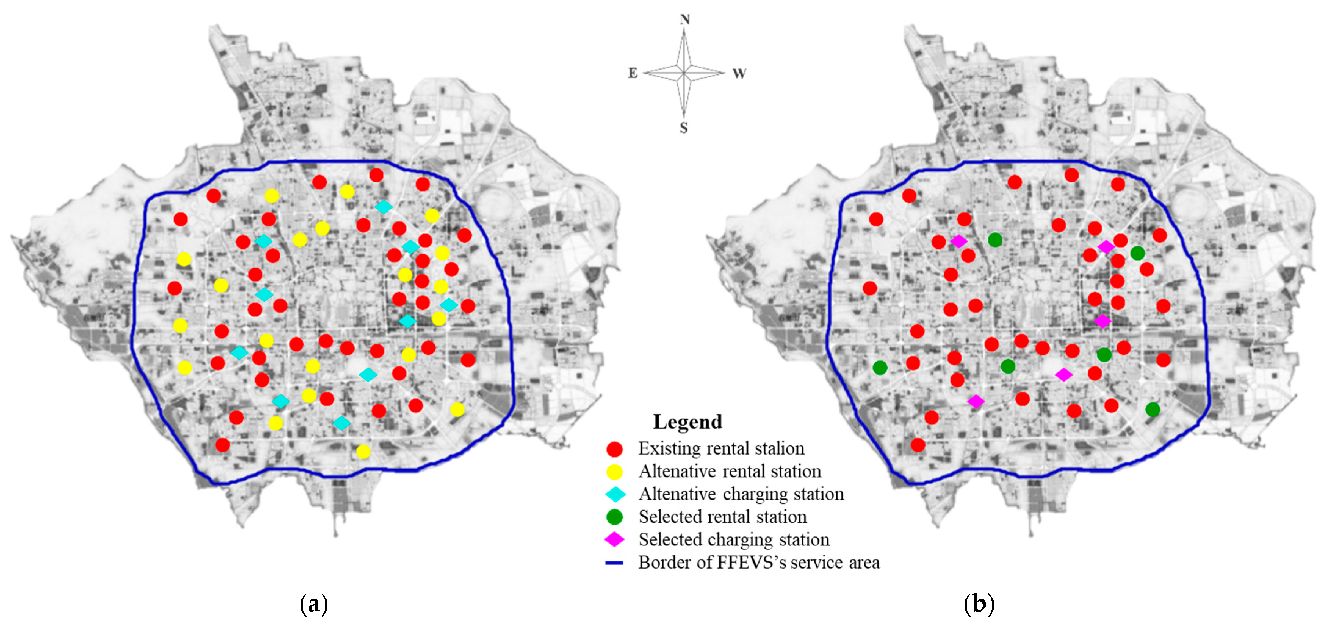
The proposed model of demand prediction and station optimization is applied to plan an FFEVS system in Beijing, China. Beijing is located between the latitudes 39°26′ N and 41°03′ N and the longitudes 115°25′ E and 117°30′ E. The study area is shown in Figure 3. It covers an area of 1.641 million hectares, including an urban area of 0.137 million hectares and a built-up land area of 0.129 million hectares. In terms of topography and geography, 38% of the area is mountainous, and the rest are plains. The total population was 21.71 million in 2021 [36].
A typical FFEVS company in Beijing is selected as a case study. The company currently has 39 main operating rental stations with 526 electric vehicles. The rental stations are mainly distributed in the main urban area of Beijing, and the type of vehicle is a Beiqi EV160 with 40 min of full charge time. To ensure vehicle performance and relocation, the rental user can use a cruising range of 130 km. New energy vehicles enjoy the purchase subsidy policy, with state subsidies of $5190 and local subsidies of $2595. The purchase cost of vehicles is $9803 per vehicle. In general, the utility time of rental vehicles is 3 years, and the selling price of each vehicle is about $1153. The cost of vehicle charging is $0.23 per kWh in Beijing, which includes a $0.115 electricity fee and a $0.115 service fee. The rental space for the FFEVS system mainly includes two aspects: the company headquarters and parking lots. The daily rental fee for the company is $0.72 per square meter. The rental price for each parking space ranges from $0.35 to $0.43, which depends on the location and flourishing degree of the parking lot where the rental stations are located.
The FFEVS system has 39 main operating rental stations, and five rental stations need to be selected from 20 alternative rental stations and four charging stations need to be selected from 10 alternative rental stations to expand the scale of the system in the main city. To cope with the enormous number of location variables, the station optimization model is used.

3.1. Data Setting

The first step is the preparation of data, which includes a considerable pre-processing work:
(1)
Apply the demand forecast model to determine the demand distribution of each electric vehicle sharing station;
(2)
geocode the potential depots for electric vehicles, using the current location of electric vehicle charging stations;
(3)
computing the travel times of the OD matrix that contains all the possible paths between depots using a GIS network shortest path algorithm with a digital elevation model. The differentiation of the shortest path for electric vehicles was included by disregarding the road altimetry variation;
(4)
computing the walking times for each candidate user from the determined location to the different potential depots.

3.2. Experimental Design

In order to select the most effective stations for the electric vehicle sharing system, several scenarios were designed and tested. These scenarios present several possible system attributes, like the station demand and the subsidy.
From the demand side, there are three possible variations: 50% decreased demand, base demand, and 50% increased demand. The second part is making the station meet future development needs. For the subsidy side, based on the government’s consideration of green travel to address the challenges of sustainable development, three different subsidy plots for sharing travel are set: 0, 0.5, and 1 dollar per hour, respectively.
By comparing the results of the above 9 combined scenarios, the 5 rental stations and 4 charging stations were the most selected in all scenarios, which is also the final solution.

3.3. Results

In this section, we will analyze the results from all the scenarios with the proposed model. The research results are shown in Table 5 and Figure 4. It is observed that (in addition to 39 already operating stations), all nine efficient solutions select stations among a set of 20 candidate rental stations and 10 charging stations. Five of these stations appear in all scenarios; thus, the five stations (codes 41, 42, 51, 54, and 55) are the final solution. Regarding the charging stations, two (codes 61 and 68) of all candidate charging stations appear in all scenarios, and another charging station appears in seven (code 63) and eight (code 67) scenarios, respectively. This result suggests that, from a station location perspective, the efficient station locations are not in conflict and the solution is robust. Since there are no conflicts in station locations, these five rental stations and four charging stations are assumed to be operating stations in further analysis.

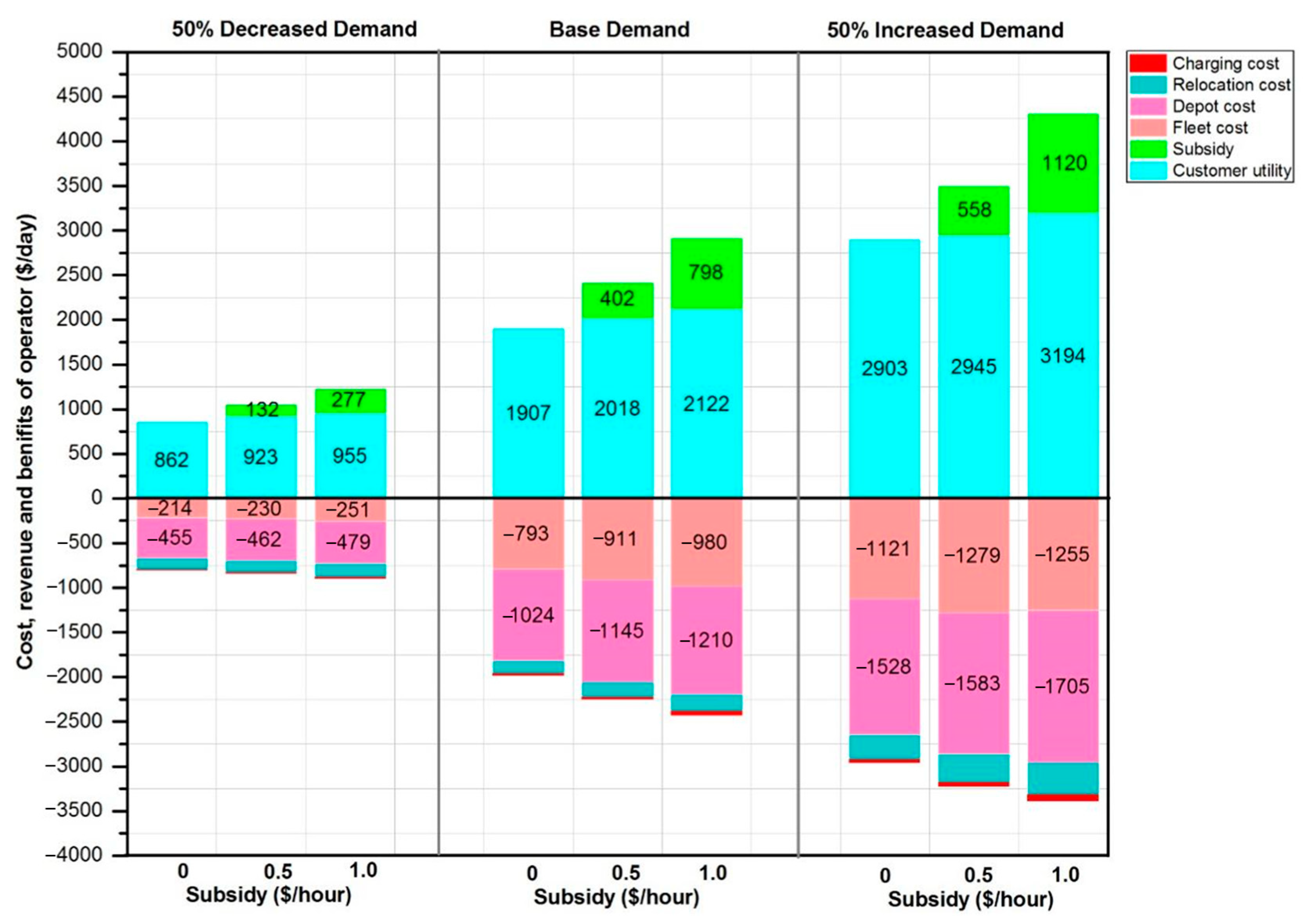
3.4. Sensitivity Analyses

The impact of subsidies holds significant importance for EVS development. By reducing the upfront costs for both operators and users, subsidies encourage the adoption of environmentally friendly vehicles, contributing to reduced carbon emissions and enhanced air quality in urban areas. It is very interesting how subsidies affect the costs, benefits, and revenues of the EVS system. Three different levels of subsidy (0, 0.5, and 1 dollars per hour) were investigated for three different levels of demand (50% decreased demand, base demand and 50% increased demand). Alternatively, if an exact model of demand sensitivity to pricing exists, a similar analysis could be made. The results of this analysis are shown in Figure 5.
The results suggest that the percentage of demand served increased from 5% to 13%. Unprofitable demand in low- or no-subsidy areas becomes profitable for the operator. Although the operator’s cost needs to increase by 4–17%, the extra revenues generated outweigh the extra costs. More importantly, the increase in subsidy has a positive effect on the number of vehicles. Since increased subsidy can enable operators to have more vehicles, the system becomes less dependent on relocation operations. Another important finding of the analysis of subsidy levels relates to the effect of the demand balance between demand level and subsidy on net revenues. When comparing the net revenues of the operator for the same subsidy with different demand levels, the increase in profit is faster than the increase in demand. It indicates that larger demand makes the system more efficient and profitable, and as a result, the level of subsidy decreases.

3.5. Compared Analyses

It is also necessary to show the advantages of the optimization algorithm. Two baselines are used here. One is a regular arrangement, where the rental stations are assigned to the centroids of a grid map. The other is a random arrangement, where the rental stations are randomly placed in the studied area. In this subsection, the area within the Third Ring Road of Beijing was used as the research object. The total number of rental stations is set at twenty.
Table 6 compares the layouts, costs, and revenue of different rental station arrangements. Compared with grid arrangements, although our method consumes more operating costs, revenue increased significantly. Specifically, our arrangement yields (647 − 252)/252 ≈ 156.7% profit growth. Unlike even distribution in random arrangements, more rental stations are placed by our method over the north of the area, to match the distribution of traffic demand. Finally, our method reduces costs by 2.7% while increasing revenue by 59.7%. The above analyses confirm that the arrangement of EVrental stations should consider user demand and operator cost jointly.

3.6. Practical Consideration

Electric vehicle sharing stands as a pivotal eco-conscious transportation solution, poised to yield substantial benefits for transportation and the environment. Nevertheless, as an emerging and evolving mode of transport, there is still a long way to go to achieve perfect integration with people’s daily lives, urban rhythms, and established transportation networks [37]. Drawing from the present study, several key policy implications are discussed herein:
(1)
Governments should comprehensively investigate the citizens’ intentions, needs, and concerns regarding the use of EVS. In combination with the survey results and the original urban development plan, each jurisdiction should formulate an EVS development plan at different levels, regions, and phases.
(2)
Operation mode of shared vehicles should be deeply combined with the space-time demand distribution of shared vehicles. The spatial demand distributions of shared cars are always related to certain interest points. The time-demand distribution of shared cars is always related to the peak travel time of residents.
(3)
Optimization of the EVS station necessitates a multifaceted perspective. In addition to in-depth consideration of traffic demand, factors such as vehicle charging, vehicle scheduling, land use, operation cost, connection with other modes of transportation, balance and optimization of traffic structure, and sustainable development should also be considered.
(4)
Policymakers should employ diverse strategies for EVS development at different stages. In the early stages of the development of electric vehicle sharing, there is great economic and market pressure and more administrative thresholds. The government can formulate preferential incentive policies in terms of subsidies, taxation, and land use. For example, prioritizing the use of roads, parking resources, and other means to support the layout of electric vehicle sharing parking spaces and charging piles.

4. Concluding Remarks

Free-floating EVS systems have emerged around the world as an alternative urban mode. These systems have been quickly evolving in the last few decades, and currently they are integrated with other existing transportation modes. This study addresses the design problem of free-floating EVS systems with EV rental stations and charging stations. The proposed model integrates demand, subsidy, and the required investment, as well as operational costs and different types of fare. The developed mathematical formulations are applied to a real-life case study. The models make a sensitivity analysis to test the influence of the considered parameters in the system design.
The carsharing demand forecasting model, based on the land characteristics of carsharing station catchment areas, proposed in the paper demonstrates good precision and can provide good support for strategic planning of shared vehicle systems. The proposed model solves the problems of existing literature by considering simultaneously decisions associated with the allocation of strategic assets, i.e., rental stations and electric vehicle charging stations for free-floating electric vehicle sharing, and the allocation of personnel for relocation operations (tactical decision). The model provides decision-makers with opportunities to perform sensitivity analyses for relevant model parameters. This feature is particularly useful for cost values that are difficult to establish empirically (e.g., utility gain from satisfied customers, population coverage, station accessibility cost). This last feature is also important if we consider that EVS systems are subsidized with public funds.
Although the model provides satisfactory results for the case under consideration, the empirical studies have concurrently illuminated certain limitations:
(1)
The study focuses on Beijing, China, which may limit the generalizability of the findings to other urban contexts with different socio-economic profiles, transportation infrastructures, or cultural attitudes towards car-sharing. Different cities have unique points of interest (POIs), population densities, and travel patterns that could influence demand forecasting differently.
(2)
While the paper uses land characteristics and POIs to forecast demand, it might not fully capture the complexity of user behavior. Factors like weather conditions, time of day, special events, public transport availability, and individual preferences can significantly affect demand but are not mentioned in the abstract.
(3)
Although a sensitivity analysis is conducted, it focuses on varying demand and subsidy levels. Other external factors such as changes in fuel prices, EV technology advancements, or shifts in government policies, could also significantly influence the effectiveness of the planning model but are not explored.
Above limitations also highlight crucial issues for further exploration in future research:
(1)
Extend the study to include multiple cities with diverse urban structures and cultural backgrounds to validate the model’s universality and refine it for better adaptability across different regions.
(2)
Integrate real-time and big data sources (e.g., social media, traffic data, weather forecasts) into the demand forecasting model to enhance accuracy and responsiveness to immediate changes in user behavior.
(3)
Develop dynamic planning models that can continuously learn and adjust station placements and fleet sizes based on real-time usage patterns and emerging trends.
(4)
Explore the influence of user psychology and behavioral economics on car-sharing adoption. Understanding user incentives, perceived convenience, and trust in technology can inform strategies to boost user engagement and loyalty.

Author Contributions

Conceptualization, Qi Cao; methodology, Qi Cao and Shunchao Wang; software, Jingfeng Ma; validation, Shunchao Wang and Jingfeng Ma; investigation, Bingtong Wang; resources, Shunchao Wang; data curation, Qi Cao and Bingtong Wang; writing—original draft preparation, Qi Cao, Shunchao Wang and Jingfeng Ma; writing—review and editing, Qi Cao; visualization, Jingfeng Ma. All authors have read and agreed to the published version of the manuscript.

Funding

This research was funded by National Science Research Foundation of China, grant number 52202399, and China Postdoctoral Science Foundation, grant number 2022M710679.

Data Availability Statement

The datasets presented in this article are not readily available because the data are part of an ongoing study. Requests to access the datasets should be directed to Shunchao Wang.

Conflicts of Interest

The authors declare no conflicts of interest.

References

  1. FHWA. Highway Statistics; Federal Highway Administration, United States Department of Transportation: Washington, DC, USA, 2022.
  2. Bureau of Transportation Statistics. Pocket Guide to Transportation; U.S. Department of Transportation: Washington, DC, USA, 2023.
  3. Li, X.; Ma, J.; Cui, J.; Ghiasi, A.; Zhou, F. Design framework of large-scale one-way electric vehicle sharing systems: A continuum approximation model. Transp. Res. Part B Methodol. 2016, 88, 21–45. [Google Scholar] [CrossRef]
  4. Sun, L.; Wang, S.; Liu, S.; Yao, L.; Luo, W.; Ashish, S. A completive research on the feasibility and adaptation of shared transportation in mega-cities—A case study in Beijing. Appl. Energy 2018, 230, 1014–1033. [Google Scholar] [CrossRef]
  5. Martin, E.; Shaheen, S. The Impacts of Car2go on Vehicle Ownership, Modal Shift, Vehicle Miles Traveled, and Greenhouse Gas Emissions: An Analysis of Five North American Cities; Transportation Sustainability Research Center: Berkeley, CA, USA, 2018. [Google Scholar]
  6. Jiao, Z.; Ran, L.; Guan, L.; Wang, X.; Chu, H. Fleet management for Electric Vehicles sharing system under uncertain demand. In Proceedings of the International Conference on Service Systems and Service Management, Dalian, China, 16–18 June 2017. [Google Scholar]
  7. Xu, F.; Liu, J.; Lin, S.; Yuan, J. A vikor-based approach for assessing the service performance of electric vehicle sharing programs: A case study in Beijing. J. Clean. Prod. 2017, 148, 254–267. [Google Scholar] [CrossRef]
  8. Bi, H.; Ye, Z.; Zhao, J.; Chen, E. Mining bike sharing trip record data: A closer examination of the operating performance at station level. Transportation 2022, 51, 1015–1041. [Google Scholar] [CrossRef]
  9. Wang, S.; Li, Z.; Wang, B.; Li, M. Collision Avoidance Motion Planning for Connected and Automated Vehicle Platoon Merging and Splitting with A Hybrid Automaton Architecture. IEEE Trans. Intell. Transp. Syst. 2024, 2, 1445–1464. [Google Scholar] [CrossRef]
  10. Illgen, S.; Höck, M. Electric vehicles in car sharing networks—Challenges and simulation model analysis. Transp. Res. Part D Transp. Environ. 2018, 63, 377–387. [Google Scholar] [CrossRef]
  11. Guillot, M.; Furno, A.; Aghezzaf, E.H.; El Faouzi, N.E. Transport network downsizing based on optimal sub-network. Commun. Transp. Res. 2022, 2, 100079. [Google Scholar] [CrossRef]
  12. Arem, B.; Azedeh, S.S.; Snelder, M.; Hoogendoorn, S. Accessibility of urban regions on a low car diet—A research agenda for digital twins. Commun. Transp. Res. 2022, 2, 100077. [Google Scholar] [CrossRef]
  13. Boyacı, B.; Zografos, K.G.; Geroliminis, N. An optimization framework for the development of efficient one-way car-sharing systems. Eur. J. Oper. Res. 2015, 240, 718–733. [Google Scholar] [CrossRef]
  14. Barth, M.; Todd, M.; Xue, L. User-based vehicle relocation techniques for multiple-station shared-use vehicle systems. Transp. Res. Rec. 2004, 1887, 137–144. [Google Scholar] [CrossRef]
  15. Biondi, E.; Boldrini, C.; Bruno, R. Optimal charging of electric vehicle fleets for a car sharing system with power sharing. In Proceedings of the 2016 IEEE International Energy Conference (ENERGYCON), Leuven, Belgium, 4–8 April 2016; pp. 1–6. [Google Scholar]
  16. Correia, G.H.D.A.; Antunes, A.P. Optimization approach to depot location and trip selection in one-way carsharing systems. Transp. Res. Part E Logist. Transp. Rev. 2012, 48, 233–247. [Google Scholar] [CrossRef]
  17. Correia, G.H.D.A.; Jorge, D.R.; Antunes, D.M. The added value of accounting for users’ flexibility and information on the potential of a station-based one-way car-sharing system: An application in Lisbon, Portugal. J. Intell. Transp. Syst. 2024, 18, 299–308. [Google Scholar] [CrossRef]
  18. Lin, J.; Chen, Q.; Kawamura, K. Sustainability SI: Logistics cost and environmental impact analyses of urban delivery consolidation strategies. Netw. Spat. Econ. 2016, 16, 227–253. [Google Scholar] [CrossRef]
  19. Hu, L.; Liu, Y. Joint design of parking capacities and fleet size for one-way station-based carsharing systems with road congestion constraints. Transp. Res. Part B Methodol. 2016, 93, 268–299. [Google Scholar] [CrossRef]
  20. Heilig, M.; Mallig, N.; Schröder, O.; Kagerbauer, M.; Vortisch, P. Implementation of free-floating and station-based carsharing in an agent-based travel demand model. Travel Behav. Soc. 2017, 12, 151–158. [Google Scholar] [CrossRef]
  21. Huang, K.; Correia, G.H.D.A.; An, K. Solving the station-based one-way carsharing network planning problem with relocations and non-linear demand. Transp. Res. Part C Emerg. Technol. 2018, 90, 1–17. [Google Scholar] [CrossRef]
  22. Ahmad, F.; Iqbal, A.; Ashraf, I.; Marzband, M. Optimal location of electric vehicle charging station and its impact on distribution network: A review. Energy Rep. 2022, 8, 2314–2333. [Google Scholar] [CrossRef]
  23. Nourinejad, M.; Zhu, S.; Bahrami, S.; Roorda, M.J. Vehicle relocation and staff rebalancing in one-way carsharing systems. Transp. Res. Part E Logist. Transp. Rev. 2015, 81, 98–113. [Google Scholar] [CrossRef]
  24. Jorge, D.; Correia, G.H.A.; Barnhart, C. Comparing optimal relocation operations with simulated relocation policies in one-way carsharing systems. IEEE Trans. Intell. Transp. Syst. 2017, 15, 1667–1675. [Google Scholar] [CrossRef]
  25. You, P.S.; Hsieh, Y.C. A study on the vehicle size and transfer policy for car rental problems. Transp. Res. Part E Logist. Transp. Rev. 2014, 64, 110–121. [Google Scholar] [CrossRef]
  26. Ataç, S.; Obrenović, N.; Bierlaire, M. Vehicle sharing systems: A review and a holistic management framework. EURO J. Transp. Logist. 2021, 10, 100033. [Google Scholar] [CrossRef]
  27. Kaspi, M.; Raviv, T.; Tzur, M.; Galili, H. Regulating vehicle sharing systems through parking reservation policies: Analysis and performance bounds. Eur. J. Oper. Res. 2016, 251, 969–987. [Google Scholar] [CrossRef]
  28. Spieser, K.; Samaranayake, S.; Gruel, W.; Frazzoli, E. Shared-vehicle mobility-on-demand systems: A fleet operator’s guide to rebalancing empty vehicles. In Proceedings of the Transportation Research Board 95th Annual Meeting, Washington, DC, USA, 10–14 January 2016. [Google Scholar]
  29. Jian, S.; Rashidi, T.H.; Wijayaratna, K.P.; Dixit, V.V. A Spatial Hazard-Based analysis for modelling vehicle selection in station-based carsharing systems. Transp. Res. Part C Emerg. Technol. 2016, 72, 130–142. [Google Scholar] [CrossRef]
  30. Sun, D.; Chen, S.; Zhang, C.; Shen, S. Bus route evaluation model based on GIS and super-efficient data envelopment analysis. Transp. Plan. Technol. 2016, 39, 407–423. [Google Scholar] [CrossRef]
  31. Wang, S.; Sun, L.; Rong, J.; Hao, S.; Luo, W. Transit trip distribution model considering land use differences between catchment areas. J. Adv. Transp. 2016, 50, 1820–1830. [Google Scholar] [CrossRef]
  32. Guo, Y.; Kelly, J.A.; Clinch, J.P. Variability in total cost of vehicle ownership across vehicle and user profiles. Commun. Transp. Res. 2022, 2, 100071. [Google Scholar] [CrossRef]
  33. Wang, S.; Ma, J.; Cao, Q.; Wang, L. Environmental Benefits and Supply Dynamics of Electric Vehicles Sharing: From A Systematic Perspective of Transportation Structure and Trip Purposes. Transp. Res. Part D Transp. Environ. 2024, 130, 104193. [Google Scholar] [CrossRef]
  34. Wang, S.; Song, Z. Exploring the Behavioral Stage Transition of Traveler’s Adoption of Carsharing: An integrated choice and latent variable model. J. Choice Model. 2024, 51, 100447. [Google Scholar] [CrossRef]
  35. Liu, Y.; Wu, F.; Liu, Z.; Wang, K.; Wang, F.; Qu, X. Can language models be used for real-world urban-delivery route optimization? Innovation 2023, 4, 100520. [Google Scholar] [CrossRef] [PubMed]
  36. Beijing Transportation Institute. Beijing Traffic Development Annual Report. 2021. Available online: https://www.bjtrc.org.cn/List/index/cid/7.html (accessed on 5 November 2018).
  37. Liu, Y.; Jia, R.; Ye, J.; Qu, X. How machine learning informs ride-hailing services: A survey. Commun. Transp. Res. 2022, 2, 100075. [Google Scholar] [CrossRef]
Figure 1. Framework.
Ijgi 13 00233 g001
Figure 2. Sketch map of points of interest distribution and grasp.
Ijgi 13 00233 g002
Figure 3. Study area.
Ijgi 13 00233 g003
Figure 4. Spatial distribution of the rental and charging stations. (a) Alternative station distribution; (b) selected station distribution.
Ijgi 13 00233 g004
Figure 5. The costs, benefits, and revenues for different subsidy and demand levels.
Ijgi 13 00233 g005
Table 1. Some related studies about the station location planning of carsharing.
ReferenceResearch ObjectResearch ContentsResearch Method
[13]EVSFleet size, the number and location of the required stations.A multi-objective mixed integer linear programming with maximization of the net revenue for both operator and users.
[16]CarsharingThe best number, location and capacities of stations.An MIP model with the objective of the maximization of the operator’s profits.
[17]CarsharingLocation of rental station, vehicle fleet size.An MIP optimization model considering trips and station locations are freely selected by the system for profit maximization.
[18]EVSLocation of rental station, vehicle inventories, system framework.A CA approach basically approximates each local neighborhood of a space with an infinite homogeneous plane (IHP),
[19]CarsharingFleet size, reservation policy, parking capacity.A mixed queuing network model with consideration of road congestion and booking policy.
[20]CarsharingTravel demand An agent-based travel demand model integrating station-based and free-floating carsharing
[21]CarsharingLocation of rental station, station capacity and fleet size problemA MILP model aims to maximize the daily profit of the carsharing operator.
[22]CarsharingVehicle fleet size and relocation, spatiotemporal demandA spatial decision support system that assists operators in countering imbalances between supply and demand.
[23]CarsharingVehicle relocation and staff rebalancingA joint optimization model for vehicle relocation and staff rebalancing using two integrated m-TSP formulations.
[24]CarsharingVehicle relocationA mathematical programming and a simulation model with the profitability of the CSO
[25]CarsharingFleet size and vehicle transferA constrained nonlinear integer-programming model within an environment of dynamic demand
[26]CarsharingLocation of rental station, vehicle fleet size.An MIP approach accounts for vehicle stock imbalances by relocating vehicles at the end of the day.
[27]CarsharingStation and vehicle parkingA MILP approach based on network flow model
[28]CarsharingFleet size and vehicle relocationA simulation approach where the actual rental data of a free-floating carsharing system is embedded
[29]CarsharingStation and vehicle selectionA behavioral model to gain a greater understanding of users’ selecting vehicles.
Table 2. Fields and example records of orders.
Station of OriginBooking TimeOrder AmountPicking Up TimeDropping Off TimeStation of
Destination
120:38:59 27.3420:49:42 21:12:43 B1
A220:41:21 37.0321:11:19 21:42:10 B2
A320:42:08 57.5120:42:20 22:28:23 B3
A420:43:33 58.3421:01:52 23:42:50 B4
A520:44:40 18.6520:45:02 23:11:08 B5
Table 3. Index significance of the demand models.
R 2 Sig.
A t i P a i B i P o i L i j A i
P i 0.8180.0000.7830.0840.022--
A i 0.7350.0000.0010.1030.015--
P s i 0.7650.0000.8490.2230.006--
P r i 0.7720.0000.7930.1000.126--
R i j 0.772-0.1240.1300.0890.0010.000
Table 4. Station demand prediction estimation model validation result.
Station242526272829Mean
Error
Model
P i −14.10%0.60%−10.30%2.90%−17.90%−14.40%10.05%
A i −11.31%4.62%12.44%−8.13%11.61%−13.25%10.23%
P s i −18.26%20.24%13.28%26.02%18.43%−6.35%17.08%
P r i 10.27%18.75%−8.74%−1.17%−6.19%18.08%10.53%
R i j 12.32%9.85%−7.44%16.74%−14.66%−8.21%11.54%
Table 5. The results of model output.
Research ScenariosRental Station SetCharging Station Set
CodeDemandSubsidy (RMB/h)
Scenario 1−50%0{41, 42, 47, 51, 54, 55, 58}{61, 63, 64, 67, 68, 70}
Scenario 2−50%3{41, 42, 46, 51, 54, 55, 58}{61, 62, 63, 64, 67, 68}
Scenario 3−50%6{41, 42, 46, 51, 53, 54, 55}{61, 64, 65, 67, 68, 69}
Scenario 4Base0{41, 42, 43, 51, 54, 55, 58}{61, 63, 65, 67, 68, 70}
Scenario 5Base3{41, 42, 43, 51, 52, 54, 55}{61, 63, 64, 66, 67, 68}
Scenario 6Base6{41, 42, 44, 51, 54, 55, 58}{61, 63, 64, 66, 68, 69}
Scenario 7+50%0{41, 42, 47, 51, 54, 55, 56}{61, 62, 63, 64, 67, 68}
Scenario 8+50%3{41, 42, 44, 51, 54, 55, 56}{61, 63, 64, 66, 67, 68}
Scenario 9+50%6{41, 42, 44, 51, 53, 54, 55}{61, 62, 65, 64, 67, 68}
Table 6. Layouts, cost, and revenue of different rental station arrangements.
Grid ArrangementRandom ArrangementOur Method
Layouts *Ijgi 13 00233 i001Ijgi 13 00233 i002
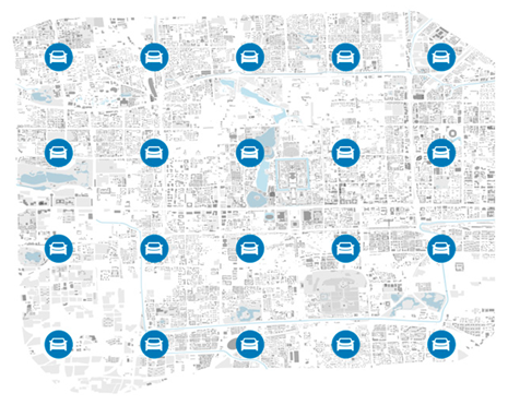
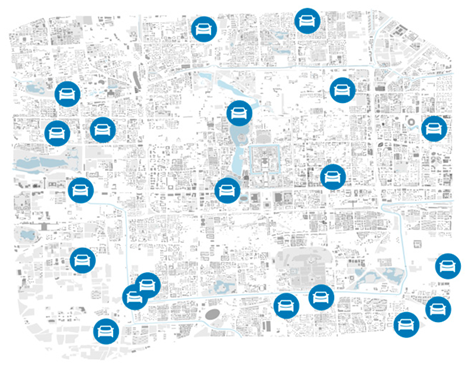
(One example of five trials)
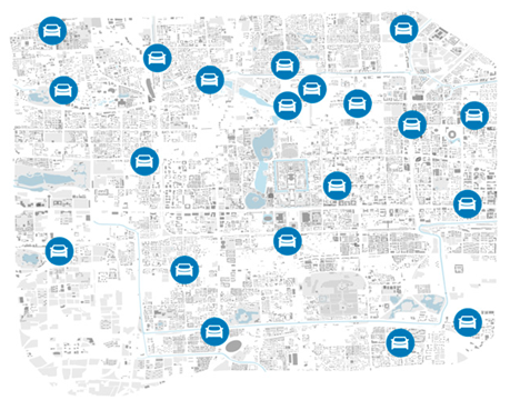
Ijgi 13 00233 i003
Cost (RMB/day)−1750−2231
(average value of five trials)
−2170
Revenue
(RMB/day)
20021764
(average value of five trials)
2817
* Ijgi 13 00233 i004 EVS station.
Disclaimer/Publisher’s Note: The statements, opinions and data contained in all publications are solely those of the individual author(s) and contributor(s) and not of MDPI and/or the editor(s). MDPI and/or the editor(s) disclaim responsibility for any injury to people or property resulting from any ideas, methods, instructions or products referred to in the content.

