Abstract
Airborne laser technology produces point clouds that can be used to build 3D models of buildings. However, the work is a laborious process that could benefit from automation. Artificial intelligence (AI) has been widely used in automating building segmentation as one of the initial stages in the 3D modeling process. The algorithms with a high success rate using point clouds for automatic semantic segmentation are random forest (RF) and PointNet++, with each algorithm having its own advantages and disadvantages. However, the training and testing data to develop and test the model usually share similar characteristics. Moreover, producing a good automation model requires a lot of training data, which may become an issue for users with a small amount of training data (limited data). The aim of this research is to test the performance of the RF and PointNet++ models in different regions with limited training and testing data. We found that the RF model developed from a small amount data, in different regions between the training and testing data, performs well compared to PointNet++, yielding an OA score of 73.01% for the RF model. Furthermore, several scenarios have been used in this research to explore the capabilities of RF in several cases.
1. Introduction
In recent years, the 3D city model has been widely used in many fields, especially the use of 3D building models for the purpose of 3D property valuation in fiscal cadastre [1,2], population estimation [3], city planning [4], cultural heritage [5,6], disasters [7], etc. The data sources required to build a 3D model vary from 2D polygons, orthophotos, and point clouds, which are closely related to its acquisition technology capabilities. Current technology is able to provide 3D data in the form of point clouds, which is capable of obtaining higher details of 3D digital models. Point clouds can be acquired using terrestrial laser scanning [8], airborne laser scanning [9], or with a combination of both [10]. Recently, airborne laser technology has become quite popular because it is inexpensive but capable of producing point clouds for the 3D modeling of buildings with a higher level of detail (LOD). However, building a 3D digital model at a high LOD using point clouds is a tedious process, for example, in establishing a 3D building model at LOD3 [4]. Therefore, an automation process is required.
The automation of modeling 3D buildings from point clouds has begun to be implemented by utilizing AI approaches in computer vision. A non-rule-based AI system is being developed, which is utilized in the automatic semantic segmentation process, for the early stages of a 3D modeling phase. The success of the initial stages in a 3D modeling process is important for the success of automation in subsequent stages, such as in the segmentation stage. The fully convolutional network (FCN), PointNet++, PointNet, and dynamic graph convolutional neural network (DGCNN) algorithms, as algorithms using the deep learning (DL) approach, already succeed in segmenting 3D data into building components [11,12,13,14]. Even though the DL approach is a further development of the ML approach in AI, its success depends on the quality and amount of available training data [15,16]. Meanwhile, machine learning (ML) has been proven to work effectively in a variety of scenarios [11], but it still produces some unavoidable noise. Therefore, the success of the utilization of the ML/DL approach in the segmentation phase depends on several parameters; one of them is the amount of available training data in the DL approach.
The number of available 3D data sources is a problem in several countries. Turkey has already used large-scale map-production regulations to develop a workflow for semi-automatic 3D city model generation [17], the Netherlands already has a 3D model of all 9.9 million buildings [3], and the Institut Cartogràfic i Geològic de Catalunya (ICGC), as the mapping agency in Catalonia, Spain, obtained 3D information by utilizing LiDAR (light detection and ranging) in urban areas [18]. Meanwhile, countries in Asia are still developing 3D city models on every available data source for various purposes. For example, Malaysia and Singapore integrated a 2D cadastral geographical dataset with 3D semantic information into a 3D model [19,20]. However, in Indonesia, the regulation of 3D model usability has only just begun, due to the limited number of 3D data sources, which leads to difficulty in using AI for 3D modeling.
Even though the number of data sources is limited, there are several open-source datasets that can be used to build an automatic semantic segmentation model, such as KITTI, ASL, iQumulus, Oxford Robotcar, NCLT, Semantic3D, DBNet [21], and DALES [22]. Furthermore, models retrieved from open-source datasets can be found in some sources. This could be a solution for countries with a limited amount of 3D data for training or an available model while using the DL approach to conduct semantic segmentation with the primary data of the country’s area. The physical city characteristics associated with a country’s incomes [23] cause the physical characteristics to be different. Therefore, the algorithms or model must be checked first.
If DL approaches are related to the amount of data training, then ML approaches are related to feature extraction, which is proven to work effectively in various scenarios. The selected algorithms used in this research are random forest (RF) in ML approaches, because it works effectively with small spatial area size of training data [24], and PointNet++ in DL approaches, because the performance is still within the top three for the LiDAR outdoor data case, with the available trained model. PointNet++ is a DL approach that requires a large amount of training data. However, in countries with limited training data, it is also possible to use a trained model that does not require additional training data. In this study, we assess the performance of PointNet++ in our study area since it already consists of a trained model and is in the top three algorithms for the LiDAR outdoor data case. The selected algorithms and the related literature are discussed further in Section 2. Therefore, the purpose of this research is to analyze the performance of the available trained model from the PointNet++ algorithm in different regions/countries, as well as to analyze the RF algorithm with a small amount of training data (limited data). This research is expected to address the problem of automating building segmentation as one of the initial stages in the 3D modeling process with a small amount of training data.
2. Literature Review
The performance of DL approaches, including PointNet++, CNN, KPConv, and KENN, depends on the quality and the amount of available training data [11], as well as the structure of the program [25]. Regarding the spatial size of the available data, several studies have conducted experiments with the spatial data size ranging between 0.19 and 12.5 km2. The DL approach produces an overall accuracy (OA) between 73.26 and 96% (Table 1). The smallest spatial area size of data used for developing semantic segmentation in a DL approach model resulted in the lowest score of OA. Thus, a larger size of the spatial area for training and testing in the DL approach yields better segmentation quality. Meanwhile, for the RF algorithm, which is classified in ML approaches, gives satisfactory results even with a small spatial area size (Table 1). The segmentation quality of the ML approach does not always depend on the amount of data, but also the geometric features [26]. The majority of datasets used to test the algorithms in Table 1 are still within the same region, except for Hu et al. (2021), where they tested the algorithms in two scenarios, namely using training and testing data within the same and different regions [27]. The OA scores between training and testing results are similar for all algorithms. Even though the regions are different, they are still located in the same country, which may still have similar physical city characteristics. Therefore, the algorithm in DL approaches must be conducted with different training and testing data in different country, which is the objective of this research.

Table 1.
Information of dataset type, spatial area size, and segmentation quality based on several literatures.
The data can be acquired through data acquisition (primary data) or from another source (secondary data), but the type of data must be similar [31]. The secondary data can be varied and found in many sources and must have the same type of data as the primary data. The sensors on UAV have the ability to efficiently provide 3D data with low cost and high resolution [32,33]. However, UAV LiDAR can collect more data and has better accuracy than UAV photogrammetry [34]. Thus, it is used as the main data source in this study.
Apart from that, the structure of a program also influences the success of automatic segmentation. The information related to papers, codes, datasets, methods and ML evaluation, contributed by various academics and industry, can be accessed at http://paperswithcode.com (accessed on 8 December 2023). The data type, algorithm rankings, and program codes used in this study were also retrieved from this source. The popular open-source data from UAV-LiDAR is the Dayton Annotated LiDAR Earth Scan (DALES) dataset, which were acquired by the University of Dayton [18]. The KPConv algorithm has the highest accuracy in the DALES dataset. Meanwhile, the Superpoint Transformer is in second place, and PointNet++ in third place. However, the algorithm with an available program and trained model by the DALES dataset is PointNet, which is adopted in Matlab R2023a. Even though the accuracy score of PointNet++ has been ranked third since 2017, it is able to produce a model with an OA score of 95.7% and mean intersect of union (MIOU) of 68.3% [14,22] with a smaller model size compared to the KPConv algorithm. Therefore, the PointNet++ algorithm was selected for this study.
PointNet++ is a development of the Pointnet algorithm, as the initiator of the semantic segmentation algorithm on a point-based point cloud. In the PointNet++ algorithm, its capabilities have been greatly improved, as it is able to learn local geometric features [13]. However, the type of geometric features in the PointNet++ algorithm and in some other DL algorithms cannot be determined by the developer. Therefore, geometric features must be built first using the ML approach according to the developer’s knowledge before conducting the training process [11,35]. The types of geometric features can be analyzed and modified in ML approaches.
Currently, the commonly used algorithms in ML are K-nearest neighbor (KNN), multiclass support vector machine (MSVM), decision trees (DTs), data assimilation (DA), naïve Bayes classifier (NB), RF, and ensemble trees (ETs). However, based on experiments conducted by Bulut (2022), applying the RF algorithm for simple surface semantic segmentation on a point cloud contributes to better accuracy, even though the computing period is longer compared to other algorithms [36]. For simple surfaces, this algorithm is suitable for use on segment point clouds for building classes, which is the main segmentation object of this research. Other advantages of using the RF algorithm include its ability to overcome overfitting problems and that it is less sensitive to outliers [37]. Based on this description, the RF algorithm in ML and PointNet++ in DL have their respective advantages and disadvantages, so they must be tested in different regions/countries, particularly in Indonesia.
3. Materials and Methods
The experiment of this research is divided into two phases. The first experiment was performed to analyze the algorithms’ capabilities using different regions for the training and testing data. The second experiment was conducted if the RF model produced better segmentation. However, if the PointNet++ produced better segmentation, then the analysis continued and the process was stopped. If in the first experiment, RF model I yielded better results, it continued to the second experiment to produce 3 (three) RF models. In the first phase, the first RF model was trained using secondary data with 8 geometric features and no RGB values. In the second phase, the other three RF models were trained using the primary data with different scenarios, namely:
- RF model II: trained with 8 geometric features (no RGB values) and 5 object classes (object classes of trucks, powerlines, and poles are not provided in the primary data);
- RF model III: trained with 11 geometric features (with RGB values) and 5 object classes (object classes of trucks, powerlines, and poles are not provided in the primary data);
- RF model IV: trained with 11 geometric features (with RGB values) and 5 object classes (converted building walls (façades) and fences into new classes).
A flow diagram of the research methodology is illustrated in Figure 1, where RF models II–IV are produced in the second experiment. The following section provides a description of the data, the feature extraction process, which is required before RF model training, the RF and PointNet++ algorithms, and analysis.
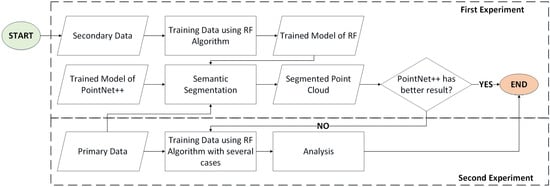
Figure 1.
Flow diagram of research methodology.
3.1. Data
3.1.1. Primary Data
Primary data were acquired using the gAirHawk GS-100C LiDAR system, covering an area of 0.083 km2 in Cimahi City, Indonesia. The LiDAR system produces a triple echo with 240,000 points/sec, and has a position accuracy of <0.056 m and measuring range of 190 m@10% reflectivity [38]. The data were stored as ‘RAW’ point clouds, which were then processed to correct the point clouds using parameters from boresight and arm-level calibration. Subsequently, a strip adjustment procedure was conducted to minimize the gaps between overlapping areas in the point clouds [39]. Then, the resulting point clouds were georeferenced to the ground control point (GCP), which was measured using a global navigation satellite system (GNSS). Coordinate transformation was carried out to transform the point cloud to the projected coordinate system. If the color (RGB value) in the point cloud was not good enough, an adjustment process was carried out using an orthophoto map, which was processed separately. The final step was to perform noise filtering using the statistical outlier removal (SOR) technique, by assuming the distances between a particular point and its neighbors were normally distributed. The points outside the 95% confidence interval were considered to be outliers [40].
The point cloud in this research produced a precision quality of 0.025 m and a density of 742 ppm. This precision value was obtained from RMSE georeferencing using four GCPs. The geometric quality of the point cloud should be obtained using independent control point (ICP). However, due to the limitations of the acquisition process, ICP measurements could not be performed. Therefore, the geometric accuracy of the point cloud could only be determined from the RMSE of the georeferenced results.
The processed point cloud of primary data was labeled manually and divided into three areas: 70% training area, 15% testing area, and 15% validation area. In the first experiment, the testing data were only used to test the PointNet++ model and RF model I. If the result met the condition, then it proceeded to the next phase using all primary datasets: training data, testing data, and validation data.
3.1.2. Secondary Data
The secondary data consist of DALES datasets and the available PointNet++ model in Matlab R2023a. The DALES dataset covers an area of 10 km2, which is divided into 29 training data files and 11 testing data files, with 8 object class categories, namely (1) land, (2) vegetation, (3) cars, (4) trucks, (5) power lines, (6) fences, (7) poles, and (8) buildings [22]. Apart from that, this point cloud does not have RGB values. A total of 8.42% of the secondary data were used to train RF model I. This consideration of spatial area size is based on the research by Zeybek (2021), which only has a small discrepancy with the spatial size of the primary training data, referred to as limited data in this research. Also, in ML, the success of the training does not depend on a greater size, but also includes a limited proportion of noise [41], wheras the secondary data are free from noise [22]. The other secondary data were from the PointNet++ model, which was been acquired from Matlab software. The PointNet++ model itself adopts the algorithm from Qi et al. (2017) and open-source DALES data from Varney et al. (2020) [42]. The model used 29 training data files, representing an area of ±7.5 km2, with 8 object class categories, similar to the original DALES dataset. The testing result produced an OA score of 93.13%, with a 89.82% accuracy score in a buildings class object.
3.2. Data Pre-Processing: Geometric Features Extraction
The data pre-processing procedure (for primary and secondary data) was conducted before the RF models’ training. The difference between ML and DL is at the feature extraction phase. In ML, before developing the model, the features must be handcrafted, which is separate from the learning. Thus, the features of the RF models/algorithm must be engineered/extracted first. Meanwhile, in DL, feature learning and model development are performed simultaneously [26].
RGB values and intensity features are the original features that can be directly obtained from the resulting point cloud. Other geometric features that are commonly used to study features in point cloud data are linearity, changes in curvature, planarity, anisotropy, and omnivariance [43] However, the omnivariance feature was excluded in this research due to its small value. These geometric features can be obtained through eigenvalues using the Gaussian elimination process to derive the eigenvector. The eigenvalues are directly proportional to the variance along the eigenvector of the covariance matrix (principal component) [44]. Therefore, these eigenvalues and eigenvectors can further explain how much the variable influences the data. This information cannot be obtained from the covariance matrix. The covariance matrix is only able to explain positive and negative relationships between variables. The order of the eigenvalue (λ1 > λ2 > λn) can be used to obtain eigenvectors as geometric features with the equations described by Blomley et al. (2014) [43].
Additionally, Zeybek (2021) added a geometric feature of height to the above ground level (AGL) [24] so that the segmentation results reach a satisfactory score of 96% OA. This height feature of AGL is widely applied as a building component segmentation parameter in point cloud data in semi-automatic techniques [45,46]. Therefore, it is sufficiently significant to be considered as a geometric feature. This research performed height feature extraction to AGL by calculating the closest distance of each point in point clouds to the digital terrain model (DTM). The DTM was obtained from a ground class that was classified using the cloth simulation filter (CSF) algorithm. The CSF algorithm is appropriate for classification on flat surfaces [47]. The CSF processing on point clouds used CloudCompare v2.12 beta [64-bit]. The AGL height was calculated using the point2trimesh() function developed by Daniel Frisch (2023) in Matlab R2023a [48] (Supplementary Materials).
3.3. Algorithms
The main algorithms used in this research were PointNet++ and random forest (RF). The operating procedures of these algorithms are as follows:
3.3.1. Random Forest (RF) Algorithm
This algorithm is a development of the ensemble tree (ET) algorithm, which uses the concept of resembling a decision tree obtained from the ensemble method, where the RF algorithm will produce many decision trees [49]. The RF algorithm uses a bagging method, which is also known as bootstrap aggregating [50]. The bagging method is an aggregation of several versions of the predicted model. Each model is trained individually and then combined using an aggregation process (averaging the results of each decision tree or taking majority voting). The main focus of bagging is to achieve less variance. In the bagging method, sample data are searched randomly from the original data for each decision tree, which is called a bootstrap sample. In each bootstrap sample dataset, there are repeated data obtained from the sampling technique with replacement. This technique helps to reduce the variance value in a set of bootstrap sample data. Each of these bootstrap samples are used for training in one decision tree. In this research, the selected parameter of the RF algorithm was performed using hyperparameter techniques to address the overfitting problem [41,51]. The parameter of the RF algorithm was the number of trees in the forest and the type of splitting data function. The numbers of trees that could be selected were 100, 200, and 300. Also, the selected splitting data function was ‘Gini’ or ‘Entropy’. The rest were default. RF processing was conducted using Python with scikit-learn as adding tools [52].
3.3.2. PointNet++ Algorithm
In general, the PointNet++ algorithm is used on point clouds by partitioning a set of points into overlapping local regions with a radius in a space-like metric [13]. Similar to the convolution neural network (CNN) algorithm, local sets of point clouds can have their local features extracted to capture geometric structures based on the local environment, which are then grouped into larger units and processed to obtain features at a higher level. This process is repeated until the features of the entire point set are obtained. The PointNet++ algorithm must be able to complete two main tasks: (1) generating partitions from a collection of point clouds and (2) abstracting the collection of points or learning local features. These two procedures are correlated because partitioning a common set of points must produce a common structure across all partitions so that they become participants in convolution, such as convolution in the CNN algorithm.
3.4. Analysis
In this step, the accuracy scores of the segmented point cloud were measured. Segmentation of point cloud was performed manually, represented as a reference point cloud. The segmented point cloud retrieved from the trained model was compared to the reference point cloud. The comparison was conducted using a confusion matrix that was built to obtain OA, recall, precision, and F1 scores as a basis for analyzing the success of each model [53]. To be able to calculate OA, recall, precision, and F1 values, a confusion matrix was required to obtain true positive (TP), true negative (TN), false positive (FP), and false negative (FN) values between the segmented point cloud and the reference point cloud. The OA value signifies the number of correct predictions out of all types of predictions composed by the model. The recall value indicates the proportion of data in the actual class (in the reference) that were correctly predicted by the model. The precision value illustrates the number of predictions that were correctly predicted in a particular class (in the reference). And the F1 score indicates the balance between precision and recall, where higher F1 scores result in more balanced recall and precision values.
4. Result
The results are divided into two sections.
4.1. First Experiment
The available PointNet++ model was used to segment the primary testing data. The visualization of the segmentation results by the PointNet++ model is shown in Figure 2. Figure 2a depicts the manually labeled primary data, whereas Figure 2b shows the segmentation results using the PointNet++ model on primary data. The visualization of the segmentation results by the RF model is shown in Figure 3. Figure 3a depicts the manually labeled primary data, whereas Figure 3b shows the segmentation results using the RF model on primary data. The point cloud, which should be segmented into building classes, produced vegetation classes instead. The OA value, precision, recall, and F1 scores of segmented point cloud were 15.7%, 5.6%, 17.3%, and 8.12%, respectively. In contrast, semantic segmentation on primary data using RF model I, which was trained with secondary data, was able to produce OA value, precision, recall, and F1 scores of segmented point clouds of 73.01%, 23.89%, 23.66%, and 23.09%, respectively (Table 2). The building class itself produced precision, recall, and F1 scores of 86.28%, 73.93%, and 79.63% (Table 2), respectively. The results of the first experiment meet the passing conditions, and so the experiment continued to the next phase. The optimal parameter of RF algorithm was 300 trees, with ‘Entropy’ as the splitting data function.
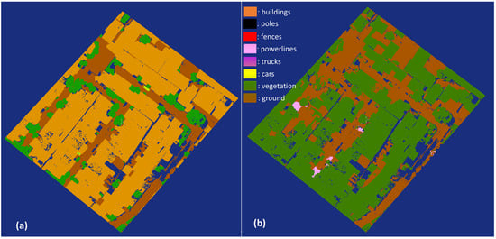
Figure 2.
Primary testing data (Cimahi City, Indonesia): (a) manual labeling; (b) semantic segmentation results of the PointNet++ model.
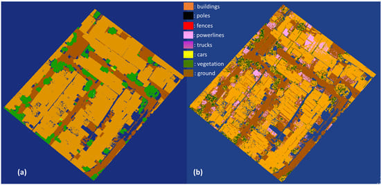
Figure 3.
Primary testing data (Cimahi City, Indonesia): (a) manual labeling; (b) semantic segmentation of RF model retrieved from trained secondary data.
Table 2.
OA, precision, recall, and F1 score of PointNet++ and RF models trained by secondary data.
Figure 4 shows the significance of geometric features on the construction of RF model I, namely the height to AGL (delta_z), normal vector to the X (normal_x), Y (normal_y), and Z (normal_z) axes, anisotropy (anisotropy), linearity (linearity), planarity (planarity), and change in curvature (c_curvature). The significant influence of geometric feature in RF model I was geometric height features on AGL (deltaz). Geometric features of RGB values are not used here because the secondary data do not have RGB values.
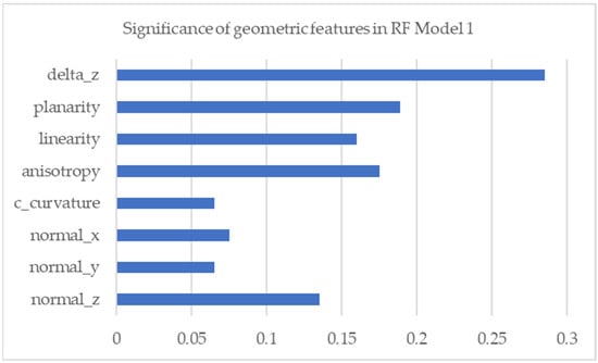
Figure 4.
Significance of geometric features in RF model I.
4.2. Second Experiment
The purpose of the second experiment was to analyze the performance of the RF algorithms. RF model II was trained with primary training data using the same geometric feature extraction as the previous experiment. The best-selected parameter number of trees was 100 and the splitting data function was ‘Gini’. Segmentation of the testing data and validation data yielded OA < 86%, precision < 48%, recall < 48%, and F1 score < 48%. The precision, recall, and F1 scores are smaller than the OA value because there are imbalance classes where car object classes are not segmented into car classes, but instead into building classes. Apart from that, the fence object class is present in the training data, but not in the testing and validation data. The segmentation results for the building class show relatively high precision, recall, and F1 scores of <90%. Appropriately, this accuracy value was increased compared to RF model I, trained by secondary data. Table 2 shows the OA, precision, recall, and F1 score values. A visualization of the semantic segmentation results of the RF 2 model is depicted in Figure 5.
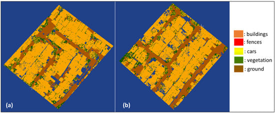
Figure 5.
Segmentation results of RF model II: (a) primary testing data; (b) primary validation data.
The RGB values are present in the primary data, but not in the secondary data. The next experiment involved the RGB values as the features in training RF model III. The results are tabulated in Table 3, and a visualization of the segmentation results of RF model III is depicted in Figure 6.
Table 3.
OA, precision, recall, and F1 score of RF model II.
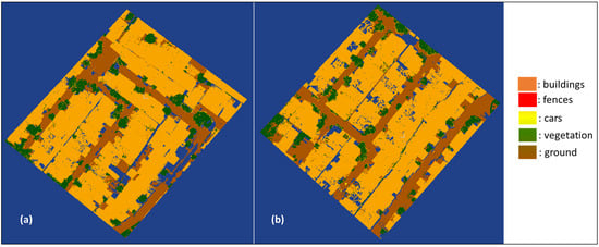
Figure 6.
Segmentation results of RF model III: (a) primary testing data; (b) primary validation data.
Table 3 indicates that there is a significant increase in the OA, precision, recall, and F1 scores compared to RF model II. Geometric features in the form of RGB values improve the performance of the RF model. Even though the OA value is <94%, which is 2% lower than the previous research conducted by Zeybek (2021), the segmentation accuracy in the building class exceeds the previous RF model. The effect of decreasing OA is due to the addition of object class in the form of cars, where the geometric features are similar to the building class. Apart from that, the significance of geometric features in the form of RGB values also has a significant influence in the construction of the RF model, where the ‘Blue’ value provides greater significance than the ‘Red’ and ‘Green’ values. The influence diagram of geometric features is shown in Figure 7.
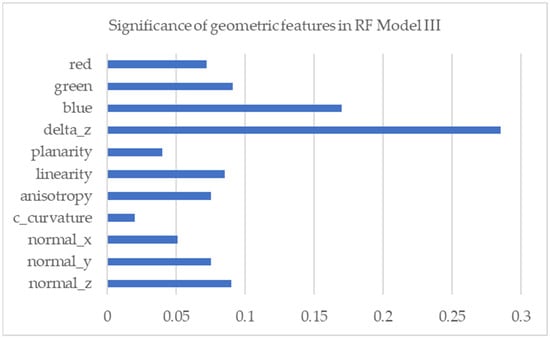
Figure 7.
Significance of geometric features of RF model III.
Another experiment was conducted by modifying the object into classes. Hypothetically, in the building class, the exterior wall of the building has different features compared to the roof, but the exterior wall has similar features to fences. Therefore, the object classes of ‘fences’ and ‘exterior wall’ became one class, as ‘exterior wall’. The next experiment was producing RF model IV with modified object classes. The accuracy values are shown in Table 4, and a visualization of the segmentation results of RF model IV is shown in Figure 8.
Table 4.
OA, precision, recall, and F1 score of RF model III.
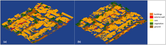
Figure 8.
Segmentation results of RF model IV: (a) primary testing data; (b) primary validation data.
In Table 5, the OA value of RF model IV decreases by 1% when compared to RF model III, but the precision and recall values increase significantly. The geometric feature of a vector normal to the Z axis increases compared to RF model III. Furthermore, the ‘Blue’ geometric feature is not as large as in RF model III. A diagrammatic visualization of the significance of geometric features on RF model IV is shown in Figure 9.
Table 5.
OA, precision, recall, and F1 score of RF model IV.
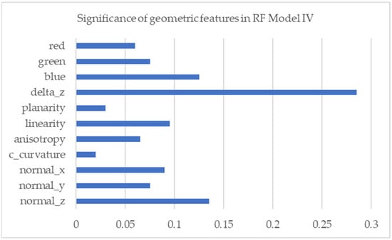
Figure 9.
Significance of geometric features of RF model IV.
5. Discussion
In the first experiment, RF model I performed better than PointNet++ (Figure 2 and Figure 3), as the spatial size of the training was similar for both models. In the second experiment (RF model II), the spatial size used for the training in the RF model was smaller than in the previous experiment (RF model I). The OA score improved by ±13% as the training spatial size was reduced significantly. When compared to the other experiment, the spatial size of the training area was the smallest, but the OA score was not ranked the lowest (Figure 10). Even though RF model II was greatly improved, the OA score was not as satisfying as in Zeybek (2021). This shows that the RF algorithm is not substantially affected by the spatial area size of the training data.
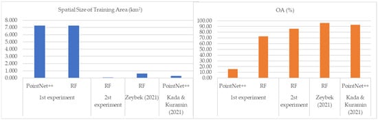
Figure 10.
Spatial size of training area (km2) and OA score of experiments [24,28].
However, the optimization parameter for RF model I and RF model II is different. In the first experiment (RF model I), the number of trees was 300, while for RF model II, it was 100. According to Zeybek (2021), the optimum number of trees for a small dataset is 50, and for larger datasets, it is >500 [24]. Different splitting data functions were used: RF model I used ‘Entropy’, and RF models II, III, and IV used ‘Gini’, based on the result of hyperparameter analysis. The differences were probably caused by different numbers of datasets.
Moreover, there is a massive discrepancy between the OA score that resulted from PointNet++ model from the first experiment and the OA score obtained by Kada and Kuramin (2021), even though the regions in the training and testing area are similar [28]. The differences in characteristic features between training data (secondary data) and testing data (primary data) were probably due the implementations in different regions. The standard deviation of the features from datasets implies variance. The highest variance of all the feature in the primary and secondary datasets was height from AGL. RF model I was most significantly influenced by height from AGL (Figure 4). The variation of features can be seen in variance values (Figure 11). Even though the variance of height from AGL in the secondary data was higher than in the primary dataset, RF model I, trained on the secondary dataset, had a higher performance than the PoinNet++ model. This indicates that the PointNet++ algorithm failed to capture the height from AGL feature, even though height is the most significant feature in the RF model. PointNet++ aggregates local features to the largest activation, hindering regional information from being fully utilized [54]. Also, the height from AGL is difficult to identify in the PointNet++ model because the height system refers to the geoid.
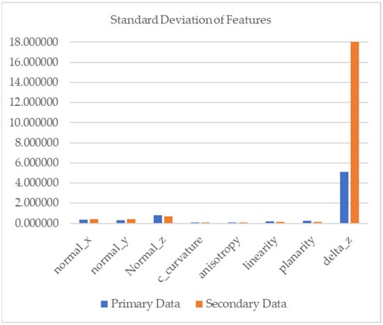
Figure 11.
Standard deviation of features of all dataset.
However, with delicate observation of the feature of the building object class (Figure 12), the variance of the features seems different (except for the feature of height from AGL). The variance of change of curvature in the primary dataset was higher than in the secondary dataset. Also, the variance of the vector normal z in the primary dataset was slightly higher than that in the secondary dataset, showing that the roof slope in primary dataset has more variety. Furthermore, the variance of change of curvature in the secondary dataset was significantly higher than the secondary dataset, showing that the roof curvature had more variety. These results indicate that the roof characteristics in the primary dataset were different from those of the secondary dataset. This is consistent with the possibility that different physical characteristics are associated with national income [23]. The different region related to the different characteristics between training data and testing data in PointNet++ model in the first experiment resulted in a huge gap with the OA score in the experiment by Kada and Kuramin (2021) [28]. Based on the explanation, the RF algorithm has higher performance than PointNet++ associated with the different characteristics of training and testing data.
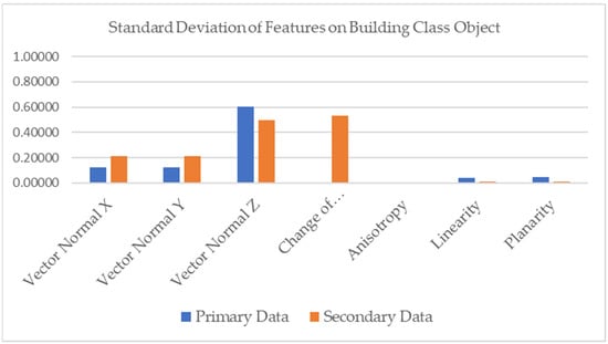
Figure 12.
Standard deviation of features on building class object.
Furthermore, the OA score in RF model III improved significantly where the RGB values were used as features in the training process. These features are similar to the experiment conducted by Zeybek (2021), which produced a similar OA score (testing and validation) in RF model III. These experiments are in tune with the statement that RGB values can significantly improve the accuracy of semantic segmentation in urban-scale scenarios [27]. Furthermore, the type of the data is different, where the primary data were from UAV LiDAR, and Zeybek (2021) used UAV images; the OA scores were not different. This indicates that the RF algorithm is also flexible to different types of data and is significantly influenced by features.
The last experiment indicated that modifying the object classes has a substantial impact on the semantic segmentation purpose. Even though the OA score in RF model IV decreased by ±2%, the accuracies (OA, precision, and F1 scores) of the roof object class (part of the building) remained the same at a ±96% OA score. The advantage is that the segmentation result can facilitate the construction of building models with LOD3, where the exterior wall object can be identified. Also, the accuracy of the exterior wall object class is around 90% (Table 4). Moreover, the significance feature in RF model IV changed from RF model III, where the vector normal z was ranked second. In the previous RF model, the significance feature of vector normal z was placed third after the ‘Blue’ value feature. This can be an advantage when RGB values are not provided in the data.
Even though this research provides a new insight into RF algorithms’ performance in semantic segmentation with small training datasets, especially in building-class objects, it also has many shortcomings. The segmented result from RF still consists of scattered noise in a class (Figure 3, Figure 5, Figure 6 and Figure 8), resulting from algorithm weakness [16], unlike the PointNet++ algorithm, which uses an autoencoder (AE) solution in DL [55]. The components of AE are encoder, decoder, and bottleneck. The adopted AE in PointNet++ consists of 3D convolutional layers, which influence the segmentation success in order to code 3D blocks. However, this is beyond the scope of this research. The convolutional 3D blocks in this research only use the default, which is 50 × 50 m in horizontal size and maximum vertical size inside the horizontal size. In PointNet++, the 3D convolutional layers are called abstraction techniques so that the structural transformation can be studied locally and globally [16,21]. Since the development of convolutional layers in the abstraction techniques in PointNet++ was not studied and developed in this research, the learning process of the PointNet++ algorithm was optimal for learning important features. Consequently, it was not optimally applied to training data and test data with different characteristics. Also, this research does not use the number of trees recommended by Zeybek (2021) related to the amount of dataset in developing the RF model. Furthermore, there are still a lot of DL algorithms that can be used and explored other than PointNet++.
6. Conclusions
The purpose of this research is to address the limited data in developing countries to accelerate the 3D modeling process using the automation technique. The main focus of this research is to analyze the possible algorithms of the opensource 3D data as training data or by using the small amount of training data to develop the automatic model. The main algorithms used in this research were PointNet++ (DL approach) and RF (ML approach).
Previous results show that the RF model outperforms the PointNet++ model in semantic segmentation where the training and testing locations are in different regions. It turns out that the features between primary (testing data) and secondary (training data) data have different building object features in height from AGL, change in curvature, and vector of normal z. Meanwhile, the size of convolutional 3D blocks in abstraction techniques uses the default, which has not been changed in this research. The convolutional 3D blocks are important in studying the local and global features in DL even though local feature learning by PointNet++ still aggregates local features simply to the largest activation.
Furthermore, the RF model is unaffected by the amount of training data but significantly related to the features. Semantic segmentation on primary testing data using an RF model trained with secondary data resulted in an OA of 73.01%, whereas the features between primary and secondary data were different. However, when the training data was replaced with similar features of the testing data, even though the amount of training data was limited, the RF algorithm still performed well in producing semantic segmentation.
Also, the performance of the RF algorithm can be increased significantly when object class categorization considers the similarity of geometric features. For example, in this research, the exterior wall and fences were categorized into one class. This can assist in developing more detailed 3D building models. However, the segmented point cloud by RF model still contained scattering noise in object class. Therefore, for further research, it is suggested to include the automation filtering of the segmented point cloud from the RF algorithm. Additionally, further research should discuss more about the size of convolutional 3D blocks in PointNet++.
Supplementary Materials
The following supporting information: (1) point2trimesh() function by Daniel Frisch (2023) can be downloaded at: https://www.mathworks.com/matlabcentral/fileexchange/52882-point2trimesh-distance-between-point-and-triangulated-surface (accessed on 20 November 2023); (2) Extension tools of random forest algorithms by scikit-learn can be downloaded at: https://scikit-learn.org/stable/modules/generated/sklearn.ensemble.RandomForestClassifier.html (accessed on 20 November 2023); (3) PointNet++ documentation can be downloaded at: Aerial Lidar Semantic Segmentation Using PointNet++ Deep Learning—MATLAB & Simulink (https://www.mathworks.com/help/lidar/ug/aerial-lidar-segmentation-using-pointnet-network.html (accessed on 20 November 2023)).
Author Contributions
Conceptualization, investigation, methodology, writing—original draft, Ratri Widyastuti; conceptualization, resources, supervision, Deni Suwardhi; supervision, Irwan Meilano and Andri Hernandi; writing—review and editing, Nabila S. E. Putri, Asep Yusup Saptari and Sudarman. All authors have read and agreed to the published version of the manuscript.
Funding
Contract number: PPMI-ITB-2023: 1219/IT1.C01.1/TA.00/2023.
Data Availability Statement
Data are unavailable due to privacy.
Acknowledgments
Secondary data, DALES (Dayton Annotated LiDAR Earth Scan) datasets were kindly provided by University of Dayton and can be found at the following link: DALES: University of Dayton, Ohio (udayton.edu). Also, the primary data were obtained using the LiDAR system provided by PT. Inovasi Mandiri Pratama. This research was funded by Penelitian, Pengabdian Masyarakat, dan Inovasi (PPMI) Program of Faculty of Earth Sciences and Technology (FITB), Institut Teknologi Bandung.
Conflicts of Interest
The authors declare no conflicts of interest.
References
- Ying, Y.; Koeva, M.; Kuffer, M.; Zevenbergen, J. Toward 3D Property Valuation—A Review of Urban 3D Modelling Methods for Digital Twin Creation. ISPRS Int. J. Geo-Inf. 2023, 12, 2. [Google Scholar] [CrossRef]
- Hendriatiningsih, S.; Hernandi, A.; Saptari, A.Y.; Widyastuti, R.; Saragih, D. Building Information Modeling (BIM) Utilization for 3D Fiscal Cadastre. Indones. J. Geogr. 2019, 51, 285–294. [Google Scholar] [CrossRef]
- Biljecki, F.; Ohori, K.A.; Ledoux, H.; Peters, R.; Stoter, J. Population estimation using a 3D City Model: A multi-scale country-wide study in the Netherlands. PLoS ONE 2016, 11, e0156808. [Google Scholar] [CrossRef]
- Ross, L.; Buyuksalih, G.; Buhur, S.; Ross, L.; Büyüksalih, G.; Baz, I. 3D City Modelling for Planning Activities, Case Study: Haydarpasa Train Station, Haydarpasa Port and Surrounding Backside Zones, Istanbul. In Proceedings of the ISPRS Hannover Workshop, Hannover, Germany, 2–5 June 2009; Available online: https://www.researchgate.net/publication/237442235 (accessed on 1 November 2023).
- Suhari, K.T.; Saptari, A.Y.; Abidin, H.Z.; Gunawan, P.H.; Meilano, I.; Hernandi, A.; Widyastuti, R. Exploring BIM-based queries for retrieving cultural heritage semantic data. Res. Sq. 2023. preprint. [Google Scholar] [CrossRef]
- Trisyanti, S.W.; Suwardhi, D.; Purnama, I.; Wikantika, K. A Preliminary Study of 3D Vernacular Documentation for Conservation and Evaluation: A Case Study in Keraton Kasepuhan Cirebon. Buildings 2023, 13, 546. [Google Scholar] [CrossRef]
- Virtriana, R.; Harto, A.B.; Atmaja, F.W.; Meilano, I.; Fauzan, K.N.; Anggraini, T.S.; Ihsan, K.T.N.; Mustika, F.C.; Suminar, W. Machine learning remote sensing using the random forest classifier to detect the building damage caused by the Anak Krakatau Volcano tsunami. Geomat. Nat. Hazards Risk 2023, 14, 28–51. [Google Scholar] [CrossRef]
- Akmalia, R.; Setan, H.; Majid, Z.; Suwardhi, D.; Chong, A. TLS for generating multi-LOD of 3D building model. IOP Conf. Ser. Earth Environ. Sci. 2014, 18, 012064. [Google Scholar] [CrossRef]
- Truong-Hong, L.; Laefer, D.F. Quantitative evaluation strategies for urban 3D model generation from remote sensing data. Comput. Graph. 2015, 49, 82–91. [Google Scholar] [CrossRef]
- Kedzierski, M.; Fryskowska, A. Terrestrial and aerial laser scanning data integration using wavelet analysis for the purpose of 3D building modeling. Sensors 2014, 14, 12070–12092. [Google Scholar] [CrossRef] [PubMed]
- Grilli, E.; Daniele, A.; Bassier, M.; Remondino, F.; Serafini, L. Knowledge Enhanced Neural Networks for Point Cloud Semantic Segmentation. Remote Sens. 2023, 15, 2590. [Google Scholar] [CrossRef]
- Yu, D.; Ji, S.; Liu, J.; Wei, S. Automatic 3D building reconstruction from multi-view aerial images with deep learning. ISPRS J. Photogramm. Remote Sens. 2021, 171, 155–170. [Google Scholar] [CrossRef]
- Qi, C.R.; Yi, L.; Su, H.; Guibas, L.J. PointNet++: Deep Hierarchical Feature Learning on Point Sets in a Metric Space. June 2017. Available online: http://arxiv.org/abs/1706.02413 (accessed on 17 May 2022).
- Kim, T.; Cho, W.; Matono, A.; Kim, K.S. PinSout: Automatic 3D Indoor Space Construction from Point Clouds with Deep Learning. In Proceedings of the ACM International Symposium on Advances in Geographic Information Systems, Seattle, WA, USA, 3–6 November 2020; Association for Computing Machinery: New York, NY, USA, 2020; pp. 211–214. [Google Scholar] [CrossRef]
- Phan, A.V.; Le Nguyen, M.; Nguyen, Y.L.H.; Bui, L.T. DGCNN: A convolutional neural network over large-scale labeled graphs. Neural Netw. 2018, 108, 533–543. [Google Scholar] [CrossRef] [PubMed]
- Grilli, E.; Poux, F.; Remondino, F. Unsupervised object-based clustering in support of supervised point-based 3D point cloud classification. Int. Arch. Photogramm. Remote Sens. Spat. Inf. Sci.—ISPRS Arch. 2021, 43, 471–478. [Google Scholar] [CrossRef]
- Buyukdemircioglu, M.; Kocaman, S.; Isikdag, U. Semi-automatic 3D city model generation from large-format aerial images. Can. Hist. Rev. 2018, 7, 339. [Google Scholar] [CrossRef]
- Stoter, J.; Vallet, B.; Lithen, T.; Pla, M.; Wozniak, P.; Kellenberger, T.; Streilein, A.; Ilves, R.; Ledoux, H. State-of-the-art of 3D national mapping in 2016. Int. Arch. Photogramm. Remote Sens. Spat. Inf. Sci.—ISPRS Arch. 2016, 41, 653–660. [Google Scholar] [CrossRef]
- Hassan, M.I.; Ahmad-Nasruddin, M.H.; Yaakop, I.A.; Abdul-Rahman, A. An Integrated 3D Cadastre-Malaysia as an Example. Int. Arch. Photogramm. Remote Sens. Spat. Inf. Sci. 2008, 37, 121–126. [Google Scholar]
- Biljecki, F. Exploration of Open Data in Southeast Asia to Generate 3D Building Models. ISPRS Ann. Photogramm. Remote Sens. Spat. Inf. Sci. 2020, 6, 37–44. [Google Scholar] [CrossRef]
- Bello, S.A.; Yu, S.; Wang, C.; Adam, J.M.; Li, J. Review: Deep learning on 3D point clouds. Remote Sens. 2020, 12, 1729. [Google Scholar] [CrossRef]
- Singer, N.M.; Asari, V.K. DALES Objects: A Large Scale Benchmark Dataset for Instance Segmentation in Aerial Lidar. IEEE Access 2021, 9, 97495–97504. [Google Scholar] [CrossRef]
- Jedwab, R.; Loungani, P.; Yezer, A. Comparing cities in developed and developing countries: Population, land area, building height and crowding. Reg. Sci. Urban Econ. 2021, 86, 103609. [Google Scholar] [CrossRef]
- Zeybek, M. Classification of UAV Point Clouds by Random Forest Machine Learning Algorithm. Turk. J. Eng. 2021, 5, 48–57. [Google Scholar] [CrossRef]
- Ramadan, T.; Islam, T.Z.; Phelps, C.; Pinnow, N.; Thiagarajan, J.J. Comparative Code Structure Analysis using Deep Learning for Performance Prediction. In Proceedings of the 2021 IEEE International Symposium on Performance Analysis of Systems and Software, ISPASS 2021, Stony Brook, NY, USA, 28–30 March 2021; Institute of Electrical and Electronics Engineers Inc.: New York, NY, USA, 2021; pp. 151–161. [Google Scholar] [CrossRef]
- Janiesch, C.; Zschech, P.; Heinrich, K. Machine learning and deep learning. Electron. Mark. 2021, 31, 685–695. [Google Scholar] [CrossRef]
- Hu, Q.; Yang, B.; Khalid, S.; Xiao, W.; Trigoni, N.; Markham, A. Towards Semantic Segmentation of Urban-Scale 3D Point Clouds: A Dataset, Benchmarks and Challenges. September 2020. Available online: http://arxiv.org/abs/2009.03137 (accessed on 2 February 2024).
- Kada, M.; Kuramin, D. ALS Point Cloud Classification using PointNet++ and KPConv with Prior Knowledge. Int. Arch. Photogramm. Remote Sens. Spat. Inf. Sci.—ISPRS Arch. 2021, 46, 91–96. [Google Scholar] [CrossRef]
- Pan, S.; Guan, H.; Chen, Y.; Yu, Y.; Gonçalves, W.N.; Junior, J.M.; Li, J. Land-cover classification of multispectral LiDAR data using CNN with optimized hyper-parameters. ISPRS J. Photogramm. Remote Sens. 2020, 166, 241–254. [Google Scholar] [CrossRef]
- Kölle, M.; Laupheimer, D.; Schmohl, S.; Haala, N.; Rottensteiner, F.; Wegner, J.D.; Ledoux, H. The Hessigheim 3D (H3D) benchmark on semantic segmentation of high-resolution 3D point clouds and textured meshes from UAV LiDAR and Multi-View-Stereo. ISPRS Open J. Photogramme-Try Remote Sens. 2021, 1, 100001. [Google Scholar] [CrossRef]
- LeCun, Y.; Bengio, Y.; Hinton, G. Deep learning. Nature 2015, 521, 436–444. [Google Scholar] [CrossRef]
- Watts, A.C.; Ambrosia, V.G.; Hinkley, E.A. Unmanned aircraft systems in remote sensing and scientific research: Classification and considerations of use. Remote Sens. 2012, 4, 1671–1692. [Google Scholar] [CrossRef]
- Colomina, I.; Molina, P. Unmanned aerial systems for photogrammetry and remote sensing: A review. ISPRS J. Photogramm. Remote Sens. 2014, 92, 79–97. [Google Scholar] [CrossRef]
- Lee, K.W.; Park, J.K. Comparison of UAV image and UAV lidar for construction of 3D geospatial information. Sens. Mater. 2019, 31, 3327–3334. [Google Scholar] [CrossRef]
- Ongsulee, P. Artificial Intelligence, Machine Learning and Deep Learning. In Proceedings of the Fifteenth International Conference on ICT and Knowledge Engineering, Bangkok, Thailand, 22–24 November 2017; IEEE: New York, NY, USA, 2017. [Google Scholar]
- Bulut, V. Classifying Surface Points Based on Developability Using Machine Learning. Eur. J. Sci. Technol. 2022, 171–176. [Google Scholar] [CrossRef]
- Ali, J.; Khan, R.; Ahmad, N.; Maqsood, I. Random Forests and Decision Trees. 2012. Available online: www.IJCSI.org (accessed on 6 May 2024).
- Geosun Geosun. Available online: https://www.geosunlidar.com/sale-13560662-geosun-gairhawk-sesries-gs-100c-lidar-scanning-system-entry-level-3d-data-collection-livox-avia-sens.html (accessed on 15 February 2024).
- Chen, H.-P.; Chang, K.-T.; Liu, J.-K. Stripe Adjustment of Airborne Lidar Data Using Ground points. In Proceedings of the Asian Conference on Remote Sensing, Pattaya, Thailand, 26–30 November 2012; Curran Associates, Inc.: Nice, France, 2012. [Google Scholar]
- Carrilho, A.C.; Galo, M.; Santos, R.C.D. Statistical outlier detection method for airborne LiDAR data. Int. Arch. Photogramm. Remote Sens. Spat. Inf. Sci. ISPRS Arch. 2018, 42, 87–92. [Google Scholar] [CrossRef]
- Ying, X. An Overview of Overfitting and its Solutions. J. Phys. Conf. Ser. 2019, 1168, 022022. [Google Scholar] [CrossRef]
- Aerial Lidar Semantic Segmentation Using PointNet++ Deep Learning. Mathworks. Available online: https://www.mathworks.com/help/lidar/ug/aerial-lidar-segmentation-using-pointnet-network.html (accessed on 15 February 2024).
- Blomley, R.; Weinmann, M.; Leitloff, J.; Jutzi, B. Shape distribution features for point cloud analysis—A geometric histogram approach on multiple scales. ISPRS Ann. Photogramm. Remote Sens. Spat. Inf. Sci. 2014, II-3, 9–16. [Google Scholar] [CrossRef]
- del Val, J.A.L.; de Agreda, J.P.A.P. Principal components analysis. Aten. Primaria/Soc. Española Med. Fam. Comunitaria 1993, 12, 333–338. [Google Scholar] [CrossRef]
- Lim, G.; Doh, N. Automatic reconstruction of multi-level indoor spaces from point cloud and trajectory. Sensors 2021, 21, 3493. [Google Scholar] [CrossRef] [PubMed]
- Shi, W.; Ahmed, W.; Li, N.; Fan, W.; Xiang, H.; Wang, M. Semantic geometric modelling of unstructured indoor point cloud. ISPRS Int. J. Geo-Inf. 2019, 8, 9. [Google Scholar] [CrossRef]
- Zeybek, M.; Şanlıoğlu, İ. Point cloud filtering on UAV based point cloud. Measurement 2019, 133, 99–111. [Google Scholar] [CrossRef]
- Frisch, D. point2trimesh()—Distance Between Point and Triangulated Surface. MATLAB Central File Exchange, 2023. Available online: https://www.mathworks.com/matlabcentral/fileexchange/52882-point2trimesh-distance-between-point-and-triangulated-surface (accessed on 17 May 2023).
- Breiman, L. Random Forests. Mach. Learn. 2001, 45, 5–32. [Google Scholar] [CrossRef]
- Breiman, L. Bagging Predictors. Mach. Learn. 1996, 24, 123–140. [Google Scholar] [CrossRef]
- Probst, P.; Wright, M.N.; Boulesteix, A.L. Hyperparameters and tuning strategies for random forest. Wiley Interdiscip. Rev. Data Min. Knowl. Discov. 2019, 9, e1301. [Google Scholar] [CrossRef]
- Buitinck, L.; Louppe, G.; Blondel, M.; Pedregosa, F.; Mueller, A.; Grisel, O.; Niculae, V.; Prettenhofer, P.; Gramfort, A.; Grobler, J.; et al. API design for machine learning software: Experiences from the scikit-learn project. In Proceedings of the ECML PKDD Workshop: Languages for Data Mining and Machine Learning, Prague, Czech Republic, 23–27 September 2013; pp. 108–122. [Google Scholar]
- Confusion Matrix—An overview—ScienceDirect Topics. Available online: https://www.sciencedirect.com/topics/engineering/confusion-matrix (accessed on 1 December 2022).
- Yan, X.; Zheng, C.; Li, Z.; Wang, S.; Cui, S. PointASNL: Robust Point Clouds Processing using Nonlocal Neural Networks with Adaptive Sampling. March 2020. Available online: http://arxiv.org/abs/2003.00492 (accessed on 1 December 2022).
- Guarda, A.F.R.; Rodrigues, N.M.M.; Pereira, F. Deep Learning-Based Point Cloud Coding: A Behavior and Performance Study. In Proceedings of the 8th European Workshop on Visual Information Processing (EUVIP), Roma, Italy, 28–31 October 2019; IEEE: New York, NY, USA, 2019; pp. 34–39. [Google Scholar]
Disclaimer/Publisher’s Note: The statements, opinions and data contained in all publications are solely those of the individual author(s) and contributor(s) and not of MDPI and/or the editor(s). MDPI and/or the editor(s) disclaim responsibility for any injury to people or property resulting from any ideas, methods, instructions or products referred to in the content. |
© 2024 by the authors. Licensee MDPI, Basel, Switzerland. This article is an open access article distributed under the terms and conditions of the Creative Commons Attribution (CC BY) license (https://creativecommons.org/licenses/by/4.0/).