Article

Genetic Programming to Optimize 3D Trajectories

1
Institute of New Imaging Technologies, Universitat Jaume I, Av. Vicent Sos Baynat, s/n, 12071 Castellón, Spain
2
Institute for Geoinformatics, University of Münster, Heisenbergstraße 2, 48149 Münster, Germany
3
NOVA Information Management School, NOVA University Lisbon, Campus de Campolide, 1099-085 Lisbon, Portugal
*
Author to whom correspondence should be addressed.
ISPRS Int. J. Geo-Inf. 2024, 13(8), 295; https://doi.org/10.3390/ijgi13080295
Submission received: 15 June 2024 / Revised: 15 August 2024 / Accepted: 19 August 2024 / Published: 20 August 2024
(This article belongs to the Special Issue Advances in AI-Driven Geospatial Analysis and Data Generation)

Abstract

:
Trajectory optimization is a method of finding the optimal route connecting a start and end point. The suitability of a trajectory depends on not intersecting any obstacles, as well as predefined performance metrics. In the context of unmanned aerial vehicles (UAVs), the goal is to minimize the route cost, in terms of energy or time, while avoiding restricted flight zones. Artificial intelligence techniques, including evolutionary computation, have been applied to trajectory optimization with varying degrees of success. This work explores the use of genetic programming (GP) for 3D trajectory optimization by developing a novel GP algorithm to optimize trajectories in a 3D space by encoding 3D geographic trajectories as function trees. The effects of parameterization are also explored and discussed, demonstrating the advantages and drawbacks of custom parameter settings along with additional evolutionary computational techniques. The results demonstrate the effectiveness of the proposed algorithm, which outperforms existing methods in terms of speed, automaticity, and robustness, highlighting the potential for GP-based algorithms to be applied to other complex optimization problems in science and engineering.

1. Introduction

1.1. Background and Problem Definition

Pathfinding essentially refers to search algorithms that connect the start and end points using a navigable path. Pathfinding in two-dimensional (2D) space or 2D routing is widely applied to navigational and logistical problems that may or may not be confined to a pathway network [1]. Increasingly complex problems are encountered in this field, especially with the introduction of additional considerations such as multiple points (Traveling Salesman Problem) [2], multiple agents (Vehicle Routing Problem) [3], or dynamism (transient obstacles, alternative routes, Dynamic Vehicle Routing Problem) [4]. Pathfinding in three-dimensional (3D) space expands upon 2D routing, with applications for autonomous or remotely operated vehicles, such as unmanned aerial vehicles (UAVs) [5,6] or unmanned underwater vehicles (UUVs) [7,8], where height and depth are, respectively, incorporated in a route or trajectory as a third spatial dimension. See Appendix A for background details.
The main advantage of 3D pathfinding is the ability to navigate in more complex environments, using routes and passages over or under no-go zones by varying altitude. An assumption in similar 2D problems is that danger zones extend to infinity in the third dimension and the results of route optimization are bound to a cost surface. However, this is not always the case [9]. With robotic vehicles becoming increasingly common and agile, the need to exploit concavities, holes, tunnels, and the spaces above and beneath structures becomes evident. Defining the extent of barriers in the third dimension allows many new routes to be considered in the optimization process.
Nevertheless, trajectory optimization in a space where transport infrastructure is irrelevant, such as aerial, submarine, subterranean, or extraterrestrial routes, is complicated by the fact that the number of possible routes is infinite [10]. The path must actively and automatically avoid physical obstacles and restricted areas, as they are implicitly avoided in pre-existing transport networks. Barrier zones around parks, hospitals, airports, or military installations may have legal, cost, or security significance. Other physical obstacles to avoid include buildings, terrain, vegetation or atmospheric phenomena. Therefore, for an exact optimization that sequentially evaluates all possible routes, it is unrealistic to find the optimum in finite time due to the immense computational resources required for “large search spaces with large numbers of potential solutions” [11] [p. 1]. Therefore, a different strategy is needed to search and sample within the solution space.

1.2. Literature Review

Evolutionary computation is an inexact, biologically inspired approach to optimization [11]. Unlike exact optimization, heuristic algorithms mimic natural evolution by testing the fitness of individuals within a population over multiple generations and applying selective pressures through a cost (or fitness) function. The procedure for finding a heuristic solution is called metaheuristics. Nature-inspired metaheuristic methods, such as evolutionary algorithms and genetic algorithms (GAs), are designed to find a good enough solution by subsampling the enormous and potentially infinite number of possible solutions in 3D space, rather than exploring them sequentially. This paper focuses on nature-inspired metaheuristic methods for spatial optimization of 3D trajectories. See Appendix B for methodological details on the literature review.

1.2.1. Trajectory Optimization Algorithms

Particle swarm optimization (PSO) [12] is the most popular technique for stochastic trajectory optimization in the related literature. For example, Mokhtari [13] generated 3D paths by mapping a B-spline to PSO-generated points and validated candidate solutions by measuring their distance from obstacles. Oultiligh et al. [14] compared Dijkstra, Voronoï, PSO, and fuzzy logic and concluded that PSO is superior because it offers the shortest possible path, while Dijkstra has difficulty in complex environments and Voronoï guarantees obstacle avoidance but cannot offer an optimal path. Other common techniques include deep learning, e.g., Qie et al. [15], to plan paths for multiple UAVs while avoiding threats.

1.2.2. 3D Trajectory Optimization

Since 3D trajectories are not restricted to pre-existing transport infrastructure, there is an additional degree of freedom as to where paths can be placed [16]. Therefore, 3D trajectory optimization is a combination of pathfinding and cost minimization. Of the nine studies that discussed 3D trajectory optimization, only five considered obstacle avoidance (see Table A1 in Appendix C). Four of them used population-based metaheuristic methods, including two swarm- and two evolutionary-based approaches. Hai-yan et al. [17] succeeded in planning multiple alternative routes with PSO. Zhang and Duan [18] used Predator-Prey Pigeon-Inspired Optimization (PPPIO) in a dynamic 3D environment, effectively incorporating a fourth dimension. Their novel algorithm is not only an improvement over PIO, but also outperformed PSO and differential evolution (DE). Evolutionary algorithms were used in the form of genetic algorithms encoding path vertices (Hildemann and Verstegen [9]) and as genetic programming encoding sequential trajectory traversal steps (Yang et al. [19]). Also with a focus on dynamic environments, Zhang et al. [20] used a semidiscretized multistep search algorithm, an improved version of A*, to successfully plan UAV stealth paths while avoiding radar.
Ma et al. [21] and Sundaran [22] emphasized the importance of path smoothness to facilitate navigation, citing the turning ability of different vehicles. Both studies used Bézier and B-spline curve generation, respectively, to obtain smoothed paths, whereas Zhang and Duan [18] used a dynamically feasible path smoothing strategy called κ -trajectories. Hildemann and Verstegen [9] also mentioned the importance of path smoothness, due to the energy loss from repeated braking and acceleration when traveling on an uneven route. In particular, in their study of trajectory optimization using genetic algorithms (GAs) for air taxis, Hildemann and Verstegen [9] (and earlier Hildemann [23]) used a directly translated chromosome to represent solutions, with individual genes consisting of the coordinates of points that compose a 3D linestring geometry. This approach, where chromosomes are lists of vertices (one point per gene), is extremely computationally demanding and has a length fixed to the number of output vertices.
Using the same evolutionary algorithm, Hildemann [23] suggested an alternative, more efficient chromosome encoding format that uses genes to encode functions, a method known as genetic programming (GP). This type of evolutionary algorithm has been applied to similar optimization problems in two [24,25] and three [5,6,19] dimensions. It differs from GA in that a program or other executable structure, rather than a sequence of coordinates, is encoded genetically. These programs are modified as the constituent genes are modified, evaluated using a cost function, and a subset of the fittest results is selected to produce the next generation. As chromosomes reproduce, genes are exchanged, combined, and mutated, and successive generations are expected to produce better solutions and evolve toward an optimal trajectory.

1.3. Research Gap

The studies above show that a great deal of research has already been invested in trajectory optimization and that several methods using artificial intelligence, including evolutionary algorithms, are currently in use. However, these methods are overwhelmingly limited to two dimensions, discontinuous space, or both. Only a small fraction of the surveyed studies venture into the third dimension and continuous space, and they find limitations in terms of speed and automaticity. Evolutionary algorithms were used in four papers: GA applied to mobile robots in 2D [26] and to UAVs in 3D [9,19], and GP applied to USVs in 2D [27]. In GP, genes are considered terms within a function, where each path represents a function. That is, solutions can be represented by syntax trees instead of vertex lists as in GA. GP-based approaches thus take advantage of function trees, which are programmatic representations and can be manipulated as genetic programs. As GP-based approaches are severely underrepresented in the existing literature, this suggests that applying GP to the 3D trajectory optimization problem is a novel approach worth investigating.

1.4. Research Questions

Given the importance of trajectory optimization in 3D environments, the main objective here is to design, implement, and evaluate a GP-based solution for 3D trajectory optimization by encoding 3D geographic trajectories as function trees and considering 3D obstacles and barriers. With the focus on chromosome representation and efficient validation, the following research questions are raised:
  • RQ1. Can functions encoding curves be effectively evolved to solve a minimization problem?
  • RQ2. How does the geometry processing method affect optimization speed?

2. Materials and Methods

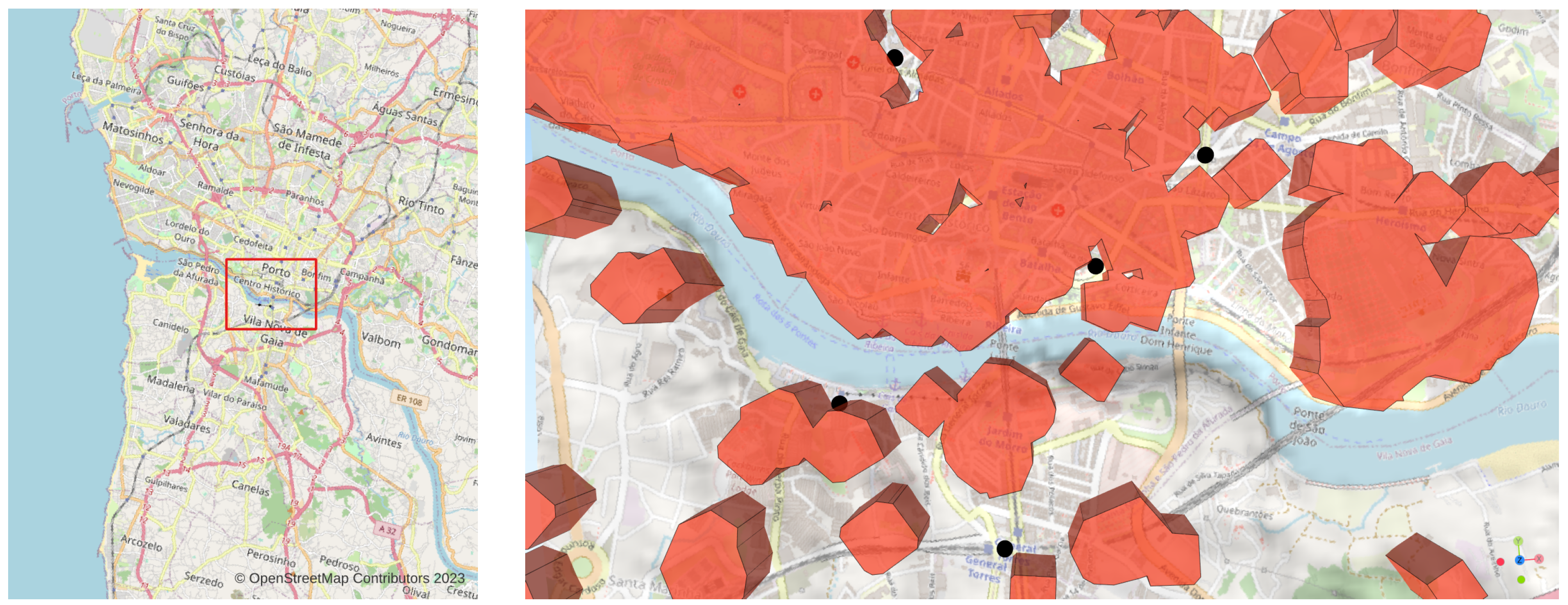
2.1. Study Area and Data Preparation

Two areas of New York City (NYC), U.S.A. (Figure 1), and one area of Porto, Portugal (Figure 2), were selected to test the route optimization solution. NYC has been previously studied for air taxi trajectory optimization [9] and Porto provides a more topographically interesting scenario. Both cities are rife with flight obstacles due to flight regulations (restricted airspace) and public disturbance (protected airspace). A fixed height above ground or sea level is the normal lower flight limit. In NYC, the Federal Aviation Administration (FAA) imposes a flight height limit due to plane air traffic of 213.36 m [28]. Preparation of the barrier dataset consisted of creating buffer zones around restricted land use areas and extruding them to the appropriate flight height clearance limits to produce 3-dimensional restricted flight zones (red polyhedrons in Figure 1 and Figure 2). Additionally, a global minimum and maximum flight altitude was specified.
The first scenario contained 17 barrier polygons around Clove Lakes Park in northern Staten Island and was prepared by manually selecting points to be used as start and end points, to provide various combinations of obstacles between pairs of points in order to assess the GP performance (Figure 1). A second scenario in NYC required navigating beyond the airport’s restricted zone near Cunningham Park, and the height limit was varied or removed to assess the optimization’s response to the changing z-dimension availability. The third scenario was central Porto and Gaia (Figure 2), in northern Portugal, and contained the deep valley of the Douro river, potentially aerially navigable.
Figure 3 illustrates the data preparation workflow for the two study areas. Data were obtained from open online sources, primarily OpenStreetMap [29] and OpenDataNYC [30], and filtered by type. Sensitive buildings and areas were then buffered laterally and vertically to create 3-dimensional restricted zones. Because intersection algorithms using simple geometries are significantly faster than algorithms using more complex meshes, barrier datasets were decomposed into their geometric primitives, such as faces, triangles, or convex hulls. For convex hulls, a barrier is intersected if any of the vertices of the 3D line are contained within the hull. The terrain representation of Porto consisted of a raster DEM, in TIFF format, and can theoretically be triangulated and sparsified for improved performance [31].

2.2. Research Methods

2.2.1. Evolutionary Computation Framework

Distributed Evolutionary Algorithms in Python (DEAP) is a Python-built framework built in Python for developing evolutionary computation techniques [32]. Function trees (syntax trees) are typified as individuals, consisting of operators and terminals (primitives) that comprise the primitive set [33]. The operators in the primitive set were selected to maximize the diversity achievable relative to the program size. Basic arithmetic functions such as addition, subtraction, multiplication, division, and negation were used in conjunction with the sine and cosine trigonometric functions to produce solution curves that can theoretically match any trajectory shape.
DEAP allows extensive customization of its internal algorithms to improve the optimization method’s performance for specific use cases, for example, when higher accuracy or speed is required, or when complex scenarios require larger trees and more iterations. Several default parameter values were derived empirically or limited due to computational constraints. Koza [34] suggested a tree height limit of 17 and a maximum number of generations of 50. Poli et al. [33] made some general recommendations while emphasizing that optimal parameters are highly application-dependent. They suggested a duration of 10 to 50 generations, stating that the most productive search occurs at this early stage and, like Koza [34], posited a population size of 500, or “as high as possible”. Table A2 in Appendix D shows default values for all parameters and describes them in detail.

2.2.2. GP Optimization Workflow

Figure 4 shows the generalized GP optimization workflow developed on top of the DEAP framework. During initialization, a starting population is randomly generated according to user-set parameters. These candidate solutions are then validated by checking whether their intersection with the barriers is an empty set. Valid solutions are then evaluated by quantifying their fitness. A cost function measures the fitness of an individual as a solution, according to the optimization criteria, and the population is subsequently ranked by fitness. The cost function returns the navigational cost of the route, which is the object of minimization, so lower fitness values mean higher suitability. With all the fitnesses known, the best-performing individual is compared to the stopping criteria. If this solution is sufficiently apt, the routine terminates and the optimization is complete; otherwise, the population is varied by mating pairs of individuals or randomly mutating genes in an individual. Individuals with better fitness (lower cost) have a higher probability of mating, mutating, or passing on to the next generation unchanged. After this variation, the offspring generated becomes the starting population of the next generation, and the process repeats. The processes of selection, crossover, and mutation are collectively referred to as genetic operators. The data and code are publicly accessible on Zenodo [35]. See Appendix E for a detailed description of each step in Figure 4.

3. Results

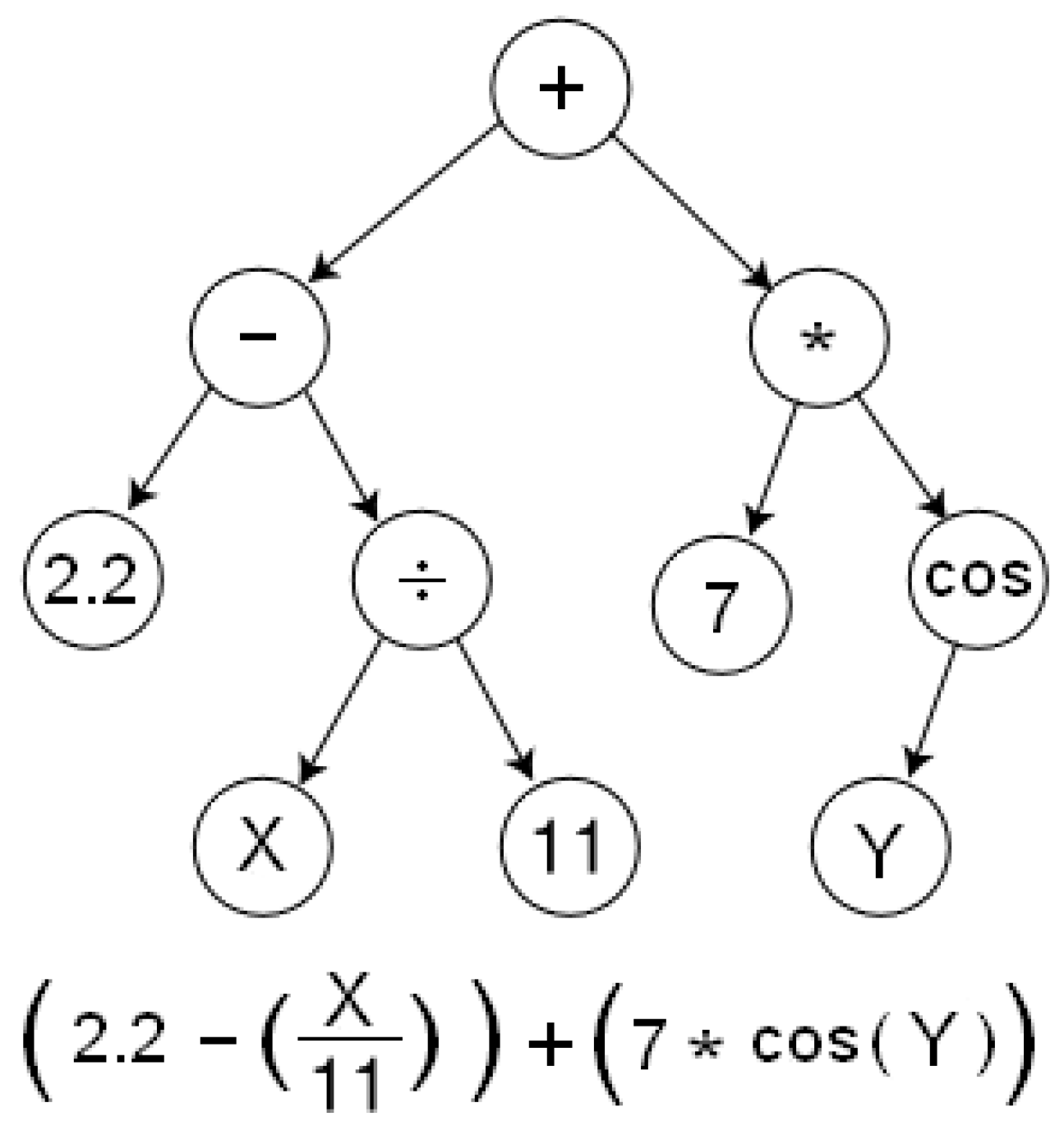
3.1. RQ1—Function Tree Representation

The GP method in 2D is robust against complex obstacle environments and usable results are obtained in a short time. The results in 3D can be faster in some cases, if a simple route over nearby obstacles is available, although the time per evaluation is longer. Considering the number of generations, the duration of 2- and 3-dimensional optimization is mainly affected by population size, geometry size (number of vertices), tree size, and scenario complexity. The quality of optimization is mainly affected by the broadness of the search, which depends on the variation and selection settings (including elitism).
Figure 5 shows two trajectories evolved to connect points b and b c . The 2D trajectory is clamped to the ground and must navigate between and around barriers, whereas the 3D trajectory can pass over barriers whenever doing so would shorten the route. Due to the innate smoothness of the generated trajectories and the weight of height minimization, the 3D route does not go over the obstacles nearest to the start and end points. Instead, it circumvents them similarly to the 2D route and only directly passes above the obstacles near the center of the trajectory.
Varying the maximum tree height shows a clear advantage for higher values in terms of fitness (Figure 6a). Note that fitness is a measure of the cost of the route and the objective is to minimize the cost. Therefore, lower fitness translates into better trajectories. In the search for local minima, there continues to be significant variability in the 95% confidence interval in subsequent generations, and the propensity for this is directly correlated with the height limit of the tree. Although evaluation time increases proportionally to tree size, the increased diversity of larger trees allows them to outperform more restricted trees. In the initial 100 generations, the median value is higher (orange line in Figure 6a), before being mostly superseded by the smallest trees until 190 generations, with the largest trees finally dominating the optimization. This suggests that parameters have distinct advantages at different stages of the evolutionary process. Lower height limits may yield quicker solutions but do so inconsistently. Higher limits ensure finer convergence, at the expense of solution size (Figure 6b) and optimization speed (Figure 6c).
Figure 7 shows the trajectories generated after 1000 generations, with quantified intersections, compared to the results of Hildemann [23] and Hildemann and Verstegen [9]. Our results are congruent with theirs with regard to the overall path. The most surprising aspect is the difference in length and smoothness: Under identical constraints (height limitation 213 m), the GP line is 12,469 m in length, compared to 12,513 m (from [9]). Although this is a minuscule reduction in length, the gradual curvature in the GP solution presents a significant reduction in flight time and energy cost due to the increased acceleration and deceleration required to navigate sharp changes in heading. In addition to the reduced computational load of the GP method, this inherent smoothness is another significant improvement over Hildemann and Verstegen [9].
Very complicated trajectories can have a huge computational cost, due to the tendency for bloating and the limited feedback available to the selection algorithm. In these cases, the optimization is nothing more than a random search. Hildemann and Verstegen [9] used a seeding method to create a progenitor trajectory that was then refined incrementally using GA and repair. Although this method works well, the seeding process requires prior knowledge of the environment. Quantifying intersection solves this problem in the scenarios tested, showing that our novel implementation outperforms Hildemann and Verstegen [9] in terms of automaticity. Although it requires significantly more time to solve, this is offset by the overall reduction in computational demand. The processing time compares extremely favorably to Hildemann [23], as shown in Table 1, where a drastic reduction in processing time is observed from hours to a few seconds over 15 generations.
Varying the global height limit also shows how the algorithm can adapt to different scenarios. In the real world, there is a flight height limit of 213 m, which forces the optimization to navigate around restricted areas of 300 m height. The 500 m limit represents a situation where the airport zone is completely impassable, but the 300 m high zone over the park can be flown over. With no global height limit, the optimal route goes directly over the airport zone (blue line in Figure 7). In the Porto–Gaia scenario, trajectories can navigate between and over restricted areas without intersecting the DEM (Figure 8).
Table 2 shows a comparison of the results of several runs, and the generations required to achieve a heuristically optimal solution with 30 generations of patience. Varied parameters are highlighted in blue.

3.2. RQ2—Geometry Processing Method

3.2.1. Initialization and Convergence

Population size is one of the two major numerical parameters of GP [34]. Poli et al. [33] recommend using the highest value that can be gracefully handled by the system in use. Figure 9 shows the outcomes of four different values for population size with all other parameters constant. As expected, it shows a clear improvement in optimization efficiency but a direct cost to evaluation time. Over 10 optimizations, larger populations converge more finely in terms of minimum fitness, but diverge more in terms of evaluation time.
Considering the stochastic nature of the initialization, variation, and selection operations, it is not surprising that optimizations with the same inputs can vary significantly. To visualize the convergence of the evolutionary process, multiple optimizations for the same problem were computed, varying the random seed state. The results show a relatively high diversity in fitness values in earlier generations, which eventually converges as the objective is reached. The 95% confidence intervals in Figure 10 show that optimizations with different starting states converge to a near-optimal solution after 50 generations for the scenario shown in Figure 10a, and 20 generations for the scenario in Figure 10b. In the third scenario, Figure 10c, the optimization fails to converge after 400 generations. Due to the complexity of this scenario, the search is vulnerable to local optima, and the initial state has a significant effect on the outcome. The minimum fitness after 400 generations ranges from 11,979 m to 25,434 m for a route with a reference theoretical minimum distance of 11,813 m.

3.2.2. Variation and Selection

Crossover and mutation directly affect the diversity of the population, which is effectively the search radius. Additionally, crossover can produce more specialized offspring by combining the beneficial traits of both parents. Figure 11 shows how optimization performance increases with a higher probability of both crossover and mutation. This illustrates how larger values allow for a quicker and broader search and may aid in avoiding or escaping local minima. Increasing these values also increases the processing time because more evaluations are required for the higher number of altered offspring.
Considering size as an additional tournament stage in the selection process means that smaller solutions are preferred if fitness is similar. Figure 12 shows the reduced average size in the double tournament experiment and a slight improvement in the optimization result.

3.2.3. Elitism

Elitism can improve the speed of convergence because it preserves the best individuals. Therefore, the population’s best fitness is protected from degradation with continued evolution. The optimization results show that the minor loss of diversity is offset by the increase in speed and quality, depending on the size of the elite fraction (see Figure 13). However, the effect is neither proportional nor consistent: after 100 generations, elitism with a 3% elite fraction outperforms 10% in terms of fitness, although 10% performs best in terms of optimization speed and solution size.
Effective bloat control using elitism is well documented [36,37], and the effect of elitism on solution size, especially in later generations, is also shown in Figure 13. After 120 generations, tree size starts to proliferate and this bloating is constrained proportionally to the elite fraction, albeit inconsistently.

3.2.4. Quantifying Validity

The first generations tend to contain more invalid solutions, and once the first valid trajectories are found, an evolutionary process of refinement centered on these trajectories is triggered. In very hard-to-navigate scenarios, with densely packed barriers or narrow passages, it is unlikely that the algorithm randomly arrives at a valid solution that can then be refined. Thus, the rough-stage optimization fails and the binary validation method is ineffective. Hildemann and Verstegen [9] circumvents this problem by “seeding” vertices within a navigable channel, and then using GA and a repair mechanism to refine this rough progenitor trajectory. This requires some foreknowledge of the barrier layout, and a more automated and potentially generalizable solution is for the algorithm to recognize such navigable channels itself. Thus, to adapt the trajectory to a highly complex airspace environment, it is necessary to drive the optimization in the right direction by providing explicit feedback. Solutions that intersect the barrier geometry to different degrees would have to be penalized differently, i.e., the validation criterion must be quantified.
Towards this end, an additional parameter was introduced to “allow” intersection. Enabling the adaptive_mode parameter means that the fitness of invalid/intersecting trajectories is not identically calculated, but depends on the amount of intersection. Trajectories that intersect barriers over most of their length will, thus, be less fit than those that intersect only in a small part. By discriminating between solutions based on the size of the intersecting set, the refining evolutionary process can begin before a valid solution is found. This refinement is then driven by incremental improvements in fitness over incremental reductions in the size of the intersecting set. The algorithm can then find more intricate solution trajectories, as it can know from the size of the intersection when it is evolving in the right direction.
Cases have been observed where optimization could not generate a valid solution due to the minimum required complexity of the solution. Figure 14 shows one example of how intersection quantification can “push” evolution towards a valid solution. This method is significantly slower because all intersections between the trajectory and barriers are measured and summed, instead of invalidating the trajectory after the first intersection is found. Since these solutions are not completely invalidated, the final solution may be invalid, having only minimized but not eliminated the amount of intersection. To avoid this, the intersection_cost parameter may be adjusted to impose a sufficient penalty to evolve away from even small intersections, towards a fully valid trajectory.
Three validation methods were developed for 3D intersections, each with their respective strengths and weaknesses. They were compared by applying the same simple trajectories within the Clove Lakes scenario. The Shapley-based2.5D method was the fastest, ranging from 20 to 50 s for a 100-generation optimization. The first SciPy-based method using Delaunay simplices was the slowest, requiring 2 to 5 hours for the same task. The second SciPy method using convex hulls required between 40 and 100 min.

4. Discussion

4.1. RQ1—Function Tree Representation

In this work, loosely typed GP is used, which allows any primitive or terminal to be passed as an argument to a primitive. Using strongly typed GP allows additional Boolean-type primitives to be incorporated. In such an implementation, conditionals such as if_then_else, operators such as xor, or Boolean terminals could also be used in the syntax tree. The efficacy of strongly typed GP applied to trajectory optimization remains to be investigated.
An alternative approach for extracting two distinct outputs from the same input to a function tree is to initialize individuals as pairs of function trees that evolve in tandem, with a single fitness value calculated for the pair. The crossover and mutation functions then need to be similarly modified to process the function pairs. This approach is more difficult to implement and tends to larger solutions, and its efficacy has not been investigated.

4.2. RQ2—Geometry Processing Method

Ideally, a population of valid trajectories would be initialized before the evolutionary process begins. Subsequent generations would then refine these individuals by adapting them more precisely to the problem. However, on highly obstructed routes it may be nearly impossible to randomly generate a valid geometry due to the complexity required. In these cases, invalid solutions are kept and their fitness is evaluated, applying a penalty proportional to the “magnitude” of their invalidity. Doing so allows the evolution to find niches or incrementally solve a very complex optimization that would not be possible without informative feedback. Another option is to seed waypoints within the navigable airspace by generating random points in the study area and using them as checkpoints for optimization.
Parameter influence was discernible to various extents and it was possible to broadly calibrate the model for different use cases by prioritizing speed, accuracy, or search radius. Certain parameters proved to be disproportionately significant, especially population size and parameters that directly improve diversity. Taking into account the test results of varying parameter values, it is possible to identify configurations that are more or less suitable for the 3D trajectory optimization problem. Population size should be as large as possible, preferably 1000 or more, and no less than 300. Size limits and variation probabilities depend on the complexity of the scenario but can be safely increased to 17 for tree height, 90% for crossover, and 25% for mutation. Elitism should be implemented with an elite fraction of 5–10%.

4.3. Applicability and Scalability

The case studies presented vary in trajectory length from 5 to 25 km and represent a common application for low-altitude routing over moderately large distances in a highly obstructed space. In the areas studied, the universal height limit has been ignored in some cases to demonstrate the ability of the method to find trajectories over restricted areas. Topographic models that incorporate terrain as an additional restriction allow for more precise pathfinding but significantly increase solving time. In two dimensions, the method can be applied to maritime routing, robot path planning, or autonomous vehicles. In three dimensions, the method can work for UAVs and submarines.
Scaling the method to much larger areas should have a very limited effect on speed, provided that the geometrical complexity is not excessive. Performance depends on the number of features and vertices within features, as well as the granularity of the trajectory and the desired coordinate precision. Geometries that are geographically larger or smaller will require the same amount of computational effort if the number of features and vertices are similar.

4.4. Comparison with Similar Methods

Compared to Hildemann [23], the optimization improved the computational requirements and allowed results to be obtained in a much shorter time. The optimization process was successful in all presented use cases and showed reliable convergence in numerous experiments. In addition, the solutions are comparatively lightweight in terms of storage and processing requirements, and the bloat-control methods implemented were able to minimize their size and maximize their processing speed.
The main improvement over Hai-yan et al. [17] and Yang et al. [19] is the complexity and density of obstacles that the new method is able to navigate through. The intrinsic trajectory smoothness also yields shorter and more efficient routes than Hai-yan et al. [17], Zhang and Duan [18], and Zhang et al. [20].

4.5. Limitations and Potential Solutions

The trend towards local optima can be effectively offset by larger population sizes and increased diversity. This directly translates into slower optimization but guarantees more consistent results despite the random nature of the initialization and variation routines. The broadness of the search and the quality of the final result rely more on the starting parameters than on the length of the optimization.
Quantifying intersections in complicated scenarios has a significant processing cost. A semiautomatic method for solving problems that require a very wide lateral or vertical deviation is to iteratively search for the nearest nonintersecting point in the plane that contains the midpoint of the start and end points of the trajectory and is normal to the line that connects them. Using the distance from this point and the displacement between the start and midpoint, a stretching factor can be calculated and used to exaggerate the route geometry in a certain direction. In this way, the algorithm could yield trajectories with very wide turns early on, allowing the rest of the optimization (refinement) to be triggered.
Where the length of intersection is measured in the evaluation routine, with adaptive_mode enabled, the algorithm is currently susceptible to errors if there are overlapping polygons. Parts of the trajectory that intersect multiple polygons will contribute to the total intersection length for each polygon. Care must be taken that no barrier geometries overlap if this setting is enabled.
A possible performance increase is the spatial indexing of barrier geometries. With this implemented, nonintersecting barriers can be identified without calling an intersection algorithm if a barrier is sufficiently distant. This can potentially speed up the validation process, which accounts for 85–95% of the processing time.
PostGIS is a popular geospatial extension for PostgreSQL that supports 3D geometries and 3D geometric predicates. Barriers can be represented as 3D polyhedral surfaces or triangulated irregular networks, and trajectories as 3D line segments [38]. It should be possible to recreate this research using geographic objects stored in a database and substituting the 3D intersection algorithm with the equivalent function in PostGIS.
Another promising prospect is meta-evolutionary algorithms, in which a GA is used to optimize the GP parameters. The calibration performed during this research could theoretically be performed more exhaustively using an evolutionary algorithm operating over repeated runs of the same optimization. Similar to this are coevolutionary algorithms that take into account multiple UAVs and have the additional condition of no collision with other UAVs while traveling along the optimized route.
The cost function can incorporate four objectives with varying weights, although the total trajectory length is the dominant fitness criterion. For improved multiobjective optimization, it is necessary to alter the method of selection to obtain a Pareto front. For example, NSGA-III is a novel nondominated sorting approach based on NSGA-II (used successfully by Hildemann and Verstegen [9] for 3D routing) that has shown its effectiveness with up to 15 objectives [39], and presents a promising research opportunity for 3D trajectory optimization in the future.

5. Conclusions

In this work, a novel approach to the trajectory optimization problem in 3D was proposed, using genetic programs to encode geometries and applying selective pressures to minimize the cost of the route while avoiding intersections with obstacles. The method was applied to case studies in New York and Porto with different levels of navigational difficulty and with different constraints imposed to assess the adaptability of the algorithm. After devising a method of evolving functions and transforming them into geographic trajectories, it was possible to evolve geographic trajectories in place and subsequently achieve the trajectory optimization goal. The syntax tree representation of functions encoding curves proved capable of representing highly variable shapes to adapt to complicated and obstacle-rich environments. These trees are also easily processed and stored, and amenable to manipulation by evolutionary processes.
In complex use cases, it was necessary to guide the evolution towards validity, since the first-generation initialization of a valid geometry becomes exceedingly unlikely in the presence of too many barriers. An adaptive method, which incorporates the intersection length into the cost function, was able to find heuristically optimal trajectories in very confined spaces. An alternative may be to construct a seed function that operates on the initialization process, to increase diversity in first-generation individual creation.
Three methods of 3D geometry intersection were compared, with a clear inverse relationship between processing speed and geometry complexity. The Shapley-based intersection evaluation method is faster but restricts the resolvable details of the third dimension. Fully 3D methods come with a significant performance cost and, as a result, may be impractical in some use cases. The 3D representation of barrier geometries is limited to convex shapes, although this only means that additional preprocessing is required to accommodate concave polyhedrons. Full support for mesh geometry is an opportunity for future work, as is the investigation into the possible benefit of GPU processing.
This research not only showcases the versatility of GP but also demonstrates the possibility of solving spatial optimization problems where the form of the solution found differs widely from the final form. The only requirement is that the solution, or an encoded form of the solution, is derivable from a function.

Author Contributions

Conceptualization, André Kotze and Moritz Jan Hildemann; methodology, André Kotze and Moritz Jan Hildemann; data curation, André Kotze and Moritz Jan Hildemann; software, André Kotze and Moritz Jan Hildemann; validation, Moritz Jan Hildemann; investigation, André Kotze; resources, André Kotze, Moritz Jan Hildemann, and Carlos Granell; writing—original draft preparation, André Kotze; writing—review and editing, Moritz Jan Hildemann, Vítor Santos, and Carlos Granell; supervision, Vítor Santos and Carlos Granell; funding acquisition, Carlos Granell. All authors have read and agreed to the published version of the manuscript.

Funding

This research is partially funded by the AICO 2023 project (grant number CIAICO/2022/111) of the Department of Innovation, Universities, Science and Digital Society of the Valencian Government, Spain.

Data Availability Statement

The data and code used in this paper are publicly accessible on Zenodo [35].

Conflicts of Interest

The authors declare no conflicts of interest.

Appendix A. Background Concepts

Pathfinding algorithms are search algorithms that aim to connect the start and end points using a navigable path. If the space in which this occurs is discretized and consists of distinct nodes connected by a finite set of edges, pathfinding is reducible to a topological problem with a finite set of possible configurations (routing in a graph). Algorithms like Dijkstra’s use exhaustive means to find a solution by repeatedly searching adjacent nodes until reaching the destination node. Artificial neural networks (ANNs), Simplex and Lagrange methods, and some heuristics including ant colony optimization (ACO), simulated annealing (SA), and particle swarm optimization (PSO) [12] have been applied to this type of routing with success. However, these methods are only applicable in discretized space (graphs). The trajectory optimization problem under consideration is continuous, following the problem formulation of Tedrake [40] and Marcucci et al. [41]: Minimizing the accumulated costs of following a trajectory in continuous space during a finite interval, i.e., from a start to an end point (Equation (A1)), subject to various constraints (Equations (A2)–(A5)). Equations (A2) and  (A4) ensure that the trajectories are derivable and within finite boundaries with a defined start, while constraints Equations (A3) and  (A5) ensure collision-free trajectories within the lower and upper height limits.
min ( · ) f ( x ( t f ) ) + t 0 t f ( ( t ) , ( t ) ) d t
x ˙ ( t ) = f ( x ( t ) , u ( t ) ) , t [ t 0 , t f ]
x ( t 0 ) = x 0
u m i n u u m a x
d 0
where:
  • t: trajectory duration,
  • x ( 0 ) : initial condition,
  • x ( t ) : initial trajectory for finite interval t,
  • u ( t ) : input trajectory for finite interval t,
  • f ( x ( t f ) ) : long term cost of following trajectory,
  • u m i n , u m a x : minimum and maximum trajectory height limits,
  • d: minimum distance of trajectory to obstacles.
Evolutionary algorithms (EAs), also known as evolutionary computation (EC), are a type of artificial intelligence that encompasses algorithms that mimic biological evolutionary processes. Global optimization is achieved via variation and selection, in the same way that species adapt to environments over generations via natural selection. At their most basic, evolutionary algorithms require genetic operators of variation (crossover and mutation) that drive the diversification into the search space, and selection pressures that guide the adaptation towards a specific goal (i.e., an adaptive system [42]). These processes of variation and selection separate a parent population from its offspring in the next generation. Genetic operators seek to randomize traits by mixing the traits of two individuals (crossover) or mutating the traits within a single individual (mutation). This diversification is made beneficial, according to the desired criteria, through the selection process. Individuals are evaluated by quantifying their fitness using a cost function and subsequently filtered to yield an offspring population that retains the best traits of their parents. Through repeated variations and selections over hundreds of thousands of generations, the solution is optimized. Genetic algorithms have been widely used for pathfinding and navigation problems in the context of optimization [43,44] and obstacle avoidance [21,45]. For example, Hu et al. [10] and Hildemann and Verstegen [9] use chromosomes that map a single gene to represent a single vertex of a linestring, which has the advantage of being simple, but can be extremely slow to process.
Figure A1. Example of a genetic program tree and the function it represents.
Ijgi 13 00295 g0a1
Genetic programming (GP) is a systematic, domain-independent automatic problem-solving method [33], which differs from genetic algorithms in that a procedure or program evolves in the optimization process. Instead of consisting of a directly encoded solution, the GP chromosome consists of an encoded function that evaluates to that solution. In linear genetic programming, evolving programs consist of a sequence of instructions processed serially. More commonly, tree-based GP is used [34], wherein programs are represented as function trees with nested subordinate trees (branches) spanning multiple levels (Figure A1). During reproduction, linear genetic programs swap out or mutate individual instructions, whereas in the case of function trees, whole nodes and branches are swapped or mutated. This implies the potential for extremely high variation in the size of function trees compared to fixed-length linear programs, and, therefore, the potential for greater diversity and faster search.

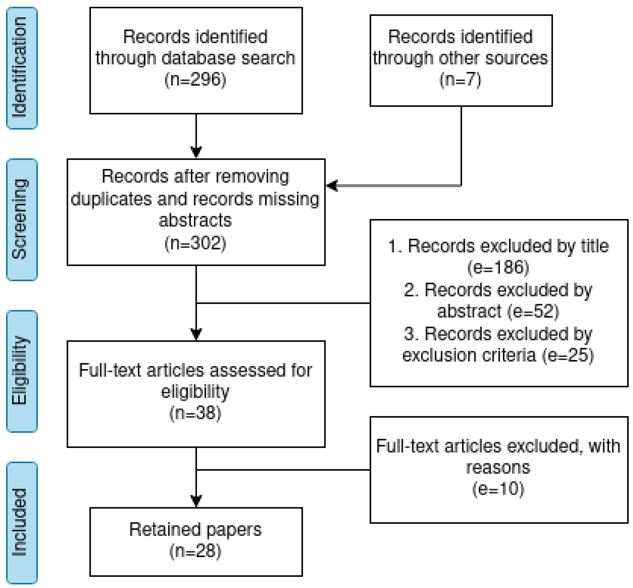
Appendix B. PRISMA Literature Review Methods

A literature review was conducted as an exploratory research step according to the Preferred Reporting Items for Systematic Reviews and Meta-Analyses (PRISMA) protocol [46]. The focus of the review was trajectory optimization in the context of 3D navigation, using artificial intelligence techniques. Therefore, the search criteria included two title-specific requirements and one more generic (title, abstract, or keywords) requirement. Firstly, results had to contain “trajectory”, “path”, or “route” as well as one of the renditions of “optimization” in the British or American spelling. To exclude outdated references, the results were also limited to papers published after 2016. The Scopus research repository was selected as the source of information and the search query below was performed in October 2022: Ijgi 13 00295 i001
Exclusion criteria were chosen to maximize the relevance of retained articles. First, optimization techniques that exclusively involved routing in noncontinuous media were identified and excluded. Second, articles that did not explicitly involve cost minimization were also excluded. Thirdly, techniques that did not require obstacle avoidance as part of the pathfinding process were excluded. Trajectory optimization in two dimensions was included since some of the techniques may still be relevant in 3D space. The results of the PRISMA systematic literature review are shown in the flow diagram in Figure A2.
Figure A2. PRISMA flowchart.
Ijgi 13 00295 g0a2
The Scopus search returned 296 results, with a further 7 sourced manually from other repositories. In these 303 records, there were no duplicates, and a single record was excluded for lacking an abstract. In total, 302 records were assessed for eligibility.
The majority of exclusions by title were on the grounds of graph-based optimization being the focus of the research. Synonyms for this domain are “combinatorial optimization”, “graph search”, etc. This includes research into air and road traffic management and robotic pathfinding in a grid-based environment. These techniques focus on node-to-node topological optimization, or optimizing the node order in a multiple-target setting.
Where the title was not sufficiently explicit to warrant exclusion, the record’s abstract was scrutinized for eligibility. In many cases, the increased detail revealed the research’s nonapplicability and a majority of rejections were again due to the research being limited to pathfinding in a graph. With 238 records already excluded by title and abstract, the remaining 63 were studied to assess relevance by consulting the full text. This process led to another 25 exclusions, leaving 38 articles for consideration in the literature review.
Of the 302 articles 106 were excluded on the basis of being routing methods that navigate through an existing network, as opposed to finding paths in an unconfined search space (regardless of dimensionality). Another 25 articles applied exclusively to routing within electronic networks. After the eligibility phase, articles were filtered a final time for valid but unanticipated reasons. Ten articles were, thus, excluded on the grounds of relevance, leaving 28 retained articles.
Regarding the 28 eligible articles, 20 articles (71%) were restricted to 2D space. Two used a cost surface as a third dimension [47,48], and one optimized the x and z dimensions [49]. The applications of the eligible studies ranged from paths for UAVs (14 records), mobile robots (7 records), USVs (2 records), and spacecraft (2 records) to UUVs, ships, and submarine pipelines (1 record each).

Appendix C. Comparison with Related Literature

Table A1. Comparison of the literature on 3D path optimization with no-fly zones.
MethodPerformance MetricsOverheadAdvantagesDisadvantages
Zhang and Duan [18]Population-based meta-heuristic: Adapted pigeon-inspired optimization and path smoothing.Composite metric including length, power consumption and constraint violation.Problem size dependent. Not specified.Applicable to moving no-fly areas.Long and exponentially increasing with increasing number of nodes in solution representation.
Zhang et al. [20]Network solving heuristic: Multistep search, Adapted A* algorithm.Detection probability, travel distance.Problem size dependent, observed: 6.13–18.48 s.Applicable to dynamic environments.Continuous 3D space is discretized into finite search space, problem size dependent computation time.
Hildemann and Verstegen [9]Population-based meta-heuristic: Adapted NSGA 2 and path smoothing.Travel time, noise emission, energy consumption.Problem size dependent, observed: 2–20 h.Applicable to highly constrained air space.Long and exponentially increasing with increasing number of nodes in solution representation.
Hai-yan et al. [17]Population-based meta-heuristic: Particle Swarm Optimization with improved K-means clustering.Terrain obstacle avoidance, detection probability, maneuverability constraints.Sufficiently efficient for pre-route planning in actual combat.Applicable to multiple alternative route planning.Rudimentary and inexact terrain obstacles. Performance only demonstrated with two alternative routes.
Yang et al. [19]Population-based meta-heuristic: Genetic programming using binary trees to encode movement increments.Problem size dependent. Not specified.Travel distance and threat avoidance.Improvement over GA applied to the same problem.Minimal exploitation of the third dimension.

Appendix D. Genetic Programming Parameters

Table A2 shows default values for all DEAP parameters. When the initial population is generated, its size is dictated by the pop_size parameter. Population size remains constant throughout the evolutionary process and directly affects diversity, with higher values having greater search potential. However, this also incurs a significant performance cost. The size of individuals is limited in length and height by the parameters max_length and max_height. These values define the maximum number of nodes in a primitive tree and the maximum depth (distance from the top of the tree to the lowest node), respectively. For example, the tree in Figure A1 (Appendix A) has a length of 10 and a height (depth) of 4. Similar to population size, larger trees encapsulate more diversity and complexity, but are detrimental to performance. The parameters init_min and init_max control the minimum and maximum length of newly initialized trees, which will have a random length within this range. Higher values may produce more complex solutions at an earlier stage in evolution.
The ngen parameter sets the number of planned generations for the optimization to evolve. This is the final stopping criterion at which point the program will terminate regardless of the quality of the optimization achieved. Alternatively, if no improvement is observed for a significant number of generations, it can be assumed that the optimization is essentially complete and no additional processing is necessary. The number of generations to wait for improvement before terminating for this reason is set by the patience parameter. Alternatively, termination can also be triggered once the first valid solution is found (useful for very complicated environments) or once the fitness reaches a specified lower threshold (useful for time-critical scenarios).
Table A2. Genetic programming parameters.
ParameterTypeDefaultDescription
pop_sizeint1000Population size
max_heightint17Size limit per individual, by number of levels
max_lengthint80Size limit per individual, by length
init_minint1Minimum length of new individuals
init_maxint2Maximum length of new individuals
mut_minint1Minimum length of new mutations
mut_maxint3Maximum length of new mutations
ngenint250Number of generations
patienceint100Number of generations to wait for improvements
cxpbfloat0.5Probability of mating two individuals
mutpbfloat0.1Probability of mutating an individual
startfloat0Starting point on reference axis
endfloat1Ending point on reference axis
nsegsint100Number of line segments in the 3D path
hof_sizeint10Number of elite individuals to preserve
elitismBoolTrueWhether to implement elitism
dbl_tournBoolFalseWhether to use two-stage tournament selection
tournsizeint3Number of individuals per tournament
parsimony_sizefloat1.7Weight of individual size in double tournament,
in the range [ 1 , 2 ]
fitness_firstBool Whether to consider fitness first during double
tournament selection, as opposed to size first
adaptive_modeBoolTrueWhether to quantify intersections
During variation, an offspring population is produced from the parent population by randomly applying crossover and mutation operations, in sequence. In the first, pairwise iteration, two consecutive individuals are crossed over (mated) according to the crossover probability parameter cxpb. After the mated individuals have been replaced by their two children, a second iteration mutates single individuals according to the probability mutpb. Higher values for the variation probability parameters lead to greater differences between parent and offspring populations.
When deriving a curve of finite length from a function tree, it is important to consider the interval in which to select the curve. The lower and upper values of the x-axis are given by the parameters start and end. The granularity of the curve, i.e., the number of vertices in the line, is given by nsegs and is one more than the number of line segments. More vertices yield a more resolved linestring but significantly affect processing speed. It is conceptually equivalent to the chromosome length in studies where lines are traditionally encoded as sequences of vertices, i.e., Hildemann and Verstegen [9], Nikolos and Brintaki [50], Yang et al. [19].
The best individuals can be selected and saved in the “Hall of Fame (HoF)”, which is updated every generation after updating their fitness. The HoF preserves the set of best solutions from the entire optimization, and individuals in the HoF can only be replaced by fitter individuals from subsequent generations. The number of solutions preserved is controlled by the hof_size parameter. While average fitness generally improves over generations, “elite” individuals with high fitness may be lost if their offspring are less fit. The stochastic nature of the optimization means that the offspring are just as likely to be better than worse. Therefore, elitism is implemented to prevent any loss of fitness by preserving elite individuals unchanged for the next generation. Therefore, elitism prevents any deterioration of the population’s maximum fitness, ensuring that the best individuals are in the final population. Elitism also has the potential to accelerate the optimization by increasing the number of pairing instances in which high-fitness individuals participate, and even counteract the propensity for bloat [37,51]. The parameter elitism determines whether elitism is implemented. In this work, elitism is enabled by default but can be disabled. Since the number of elite individuals retained per generation is determined by the hof_size parameter, the elite fraction is defined as the ratio of hof_size and pop_size. Increasing the elite fraction may be beneficial, but it also carries the risk of premature convergence due to the corresponding cost of diversity.
As a result of continuous variation over generations, the size of trees generally increases disproportionately to their fitness. This phenomenon is known as bloat [33,36] and it can dramatically reduce optimization performance. In this work, four methods of bloat control are implemented: a global hard limit on the size of trees, double tournament selection, size as part of the cost function, and an elitist strategy. The global limit suggested by Koza [34] is 17, but it allows for enormous programs up to 131 , 072 ( 2 17 ) in length. In this study, limits of 8, 12, and 17 are used in combination with other bloat control methods. To toggle between tournament selection or double tournament selection, the dbl_tourn parameter may be adjusted. The tournsize parameter determines the number of individuals participating in each tournament. The double tournament takes two additional parameters: parsimony_size defines the weight of the solution size in the second part of the tournament and must be a real number in the range [ 1 , 2 ] ;  fitness_first determines whether the fitness or size stage of the tournament is held first.
Two degrees of freedom in the pseudo-y and pseudo-z dimensions of the solution space allow individuals to develop increased complexity and a greater likelihood of finding valid trajectories in complex and obstacle-rich scenarios. These can be considered as lateral and vertical deviations from the straight line (pseudo-x) that connects the point of origin and destination. To yield these truly 3-dimensional lines, an additional input argument is added to the primitive set so that the function tree accepts two arguments. These can then be individually evaluated by setting the other value to 0 (or any other arbitrary value) to produce two distinct outputs from a single tree.
The smoothness and granularity of the solution are important factors for trajectory navigability due to the differing turning radii and attainable ascent gradients of UAVs. It is also beneficial in terms of energy cost to navigate along smoother routes [21]. Hildemann and Verstegen [9] used a set of vertices (3D points) with a corresponding set of smooth lines connecting them, whereas Ma et al. [21] used a set of control points to constrain a Bézier curve. In this work, the smoothness derives from the curve of the functions represented by the genetic programs, and the granularity depends directly on the ratio between the trajectory length and the nsegs parameter.
Finally, processing time or effort (computational complexity) strongly depends on the size of inputs, in particular the granularity of trajectory data and barrier geometry data. In adaptive_mode, the intersection algorithm evaluates the intersection between every vertex of the 3D linestring geometry and every barrier geometry in order to quantify the intersection. However, with adaptive_mode disabled, the algorithm exits after the first intersection is found. The maximum computation time outside adaptive mode is, therefore, the standard computation time in adaptive mode, and can be given by
O ( i · g · m · f )
f = ( n · k )
where:
  • g: number of generations;
  • n: number of vertices in the output trajectory;
  • m: number of barrier geometries;
  • k: average number of vertices in each barrier geometry;
  • i: number of iterations in the optimization;
  • f: complexity of the intersection test.

Appendix E. GP Optimization Workflow

Based on the workflow depicted in Figure 4, variation algorithms change the parent population into the offspring, by crossing over genes from two chromosomes, mutating individual chromosomes, or both. We use a variation that applies both crossover and mutation. The operators are not applied systematically. Rather, an initial iteration over the population pairs consecutive individuals according to the crossover probability cxpb parameter (see Table A2 in Appendix D) and the resulting individuals replace their parents. In this work, the tools.cxOnePoint algorithm is used for crossover, which only swaps a sub-branch of each tree at one point. A second iteration mutates individuals according to the mutation probability mutpb parameter, and the mutated individuals replace their unmutated versions. The mutation method used is tools.mutUniform, which selects a random point in the tree and replaces the sub-branch stemming from this point with a newly generated tree. Thus, offspring are made of new individuals that are crossed over, mutated, both, or unchanged.
After evaluating the fitness of all individuals in the population, selection is performed using tournament selection, which iteratively selects the best solution from a subset of randomly selected individuals. The double tournament has a second stage where solution size is considered, rather than fitness, and has been shown to effectively control bloat by preferring smaller individuals [52].
Figure A3. Solution transformation procedure.
Ijgi 13 00295 g0a3
The individual validation procedure starts by decoding the chromosome and compiling the program into a callable function. This function is then plotted in 3D space in an arbitrary interval to yield a finite path between two points (Figure A3). To validate this path, it is mapped directly to the problem interval in geographic space by transforming it geometrically, i.e., the curve is reprojected in three dimensions to connect the start and end points. The suitability of the resulting trajectory can then be assessed according to the chosen criteria. The transformation procedure requires the start point, end point, and a number of segments, and its steps are outlined below:
  • Translate to origin;
  • Normalize;
  • Rotate about origin;
  • Scale to geographic size;
  • Translate to destination.
To facilitate rotation (about the origin), the solution curve is translated to the origin. The coordinates of the start point are subtracted from each coordinate in the list:
Translation : v i = v i v 0 , i = 1 , 2 , , n ,
The next step is the normalization of the vector, achieved by dividing the vector by its magnitude. Here, we consider the direct (net) displacement from the start point to the end point as the vector:
Normalization : u ^ = u | u |
After normalizing, we are left with a unit vector that we want to align with the geographic displacement by rotation. Simple Euler rotation introduces error due to gimbal lock, a well-known limitation in 3D rotation using Euler angles [53] where two axes align during rotation, causing the rotational system to lose a degree of freedom. Instead, quaternion rotation is used to rotate the vector in a single direction in a single instance. Since quaternions have only four components and are applied only once, they are computationally more efficient than matrices [54] and are not susceptible to gimbal lock. The quaternion initialization requires two arguments: the overall axis of rotation in ijk space (equal to the cross product of the two unit vectors) and the angle of rotation (scalar, equal to the dot product of the two unit vectors). Once the quaternion is created, the same magnitude of rotation is applied to each vertex of the solution line to align it with the geographic interval. Here, s represents | | q | | or the rotation magnitude, and the only real component. q i , q j , and q k represent the imaginary spatial components in quaternion space:
Rotation : R = 1 2 s ( q j 2 + q k 2 ) 2 s ( q i q j q k q r ) 2 s ( q i q k + q j q r ) 2 s ( q i q j + q k q r ) 1 2 s ( q i 2 + q k 2 ) 2 s ( q j q k q i q r ) 2 s ( q i q k q j q r ) 2 s ( q j q k + q i q r ) 1 2 s ( q i 2 + q j 2 )
The penultimate step is to scale the curve to the size of the geographic interval. For this, a simple scaling matrix is used, with the scale factor k equal to the magnitude of the geographic interval divided by that of the solution curve.
Scaling : S k = k 0 0 0 k 0 0 0 k
Finally, the result is translated from the origin to map onto the geographic space, simply by adding the coordinates of the geographic start point σ 0 to each vertex of the scaled trajectory.
Translation : v i = v i + δ 0 , i = 1 , 2 , , n ,
For the path validation, the geographic path is plotted in the same space as the 3D barriers and is validated by checking whether any intersection exists between it and the barriers. There are several approaches, varying in accuracy and performance. Computational load is affected by the intersection algorithm used and the geometry representation: the solution can be considered as a collection of line segments (high computational cost) or vertices (low cost). Likewise, barriers can be considered as 3D meshes (high cost), or collections of concave hulls (medium cost), or collections of 3D polygons with a height attribute (low cost). Another possibility is to use 2D polygons with a height attribute. This has a low computational cost but limits the third dimension to a single range per polygon. Accuracy is equally affected by geometric representation. The vertices of a path may not intersect a barrier, although its segments do [9]. More intricate geometries can be represented with 3D meshes than with convex hulls or polygons.
In this work, three approaches to 3D intersection are considered. The first is a simplified two-and-a-half-dimensional (2.5D) geographic intersection, where the x–y intersecting geometry (if it exists) is evaluated separately in the z-dimension. The restricted height range is taken from the barrier data attributes. Although fast and applicable to many real scenarios, this approach is limited in its representation of complex 3D environments. The second and third approaches are fully 3-dimensional methods using convex hulls and points. Both evaluate the line vertices sequentially: one by checking whether the point lies within the Delaunay triangulation of the convex hull, and the other by creating a new convex hull that includes the point, and checking whether the two convex hulls are equal. Therefore, they are limited to convex geometries (although concave shapes can be decomposed in an additional preprocessing step) and are susceptible to omission errors due to their use of route vertices instead of line segments.
Invalid paths are deleted or their fitness is severely penalized, depending on the model configuration. Deleting invalid individuals ensures that the population only contains viable solutions that will continue to be optimized. However, as the complexity of a scenario increases, the likelihood of initializing a valid individual decreases, and it is not unusual for valid solutions to never be randomly initialized. Penalizing invalid routes signals to the model the undesirability of such routes, but allows evolution to continue refining it by allowing the individual to be varied.
After validation, paths are evaluated by calculating their fitness. The optimization objectives are incorporated into the cost function, and in this way, a ranking is established within the generation for the selection operation. The primary consideration is the total path length. Other metrics with adjustable weight include solution size and path variability in the z-dimension (with a directly associated energy cost). Path length can be measured directly in 3D, but the cost of moving through the z-dimension is not equivalent to moving parallel to the surface. Length can be measured in the x–y plane, and variation in the third dimension can be measured separately, as absolute cumulative displacement. Therefore, vertical movement will tend to be minimized and the ratio between these measurements can be adjusted.

References

  1. Garip, Z.; Karayel, D.; Erhan Çimen, M. A study on path planning optimization of mobile robots based on hybrid algorithm. Concurr. Comput. Pract. Exp. 2022, 34, e6721. [Google Scholar] [CrossRef]
  2. Pezer, D. Efficiency of tool path optimization using genetic algorithm in relation to the optimization achieved with the CAM software. Procedia Eng. 2016, 149, 374–379. [Google Scholar] [CrossRef]
  3. Baker, B.M.; Ayechew, M. A genetic algorithm for the vehicle routing problem. Comput. Oper. Res. 2003, 30, 787–800. [Google Scholar] [CrossRef]
  4. Kim, H.; Kim, S.H.; Jeon, M.; Kim, J.; Song, S.; Paik, K.J. A study on path optimization method of an unmanned surface vehicle under environmental loads using genetic algorithm. Ocean. Eng. 2017, 142, 616–624. [Google Scholar] [CrossRef]
  5. Meng, H.; Xin, G. UAV route planning based on the genetic simulated annealing algorithm. In Proceedings of the 2010 IEEE International Conference on Mechatronics and Automation, Xi’an, China, 4–7 August 2010; pp. 788–793. [Google Scholar]
  6. Wang, H.; Lyu, W.; Yao, P.; Liang, X.; Liu, C. Three-dimensional path planning for unmanned aerial vehicle based on interfered fluid dynamical system. Chin. J. Aeronaut. 2015, 28, 229–239. [Google Scholar] [CrossRef]
  7. An, P. Path Optimization Method of Autonomous Intelligent Obstacle Avoidance for Multi-joint Submarine Robot. J. Coast. Res. 2018, 82, 288–293. [Google Scholar] [CrossRef]
  8. Balicki, J. Multicriterion genetic programming for trajectory planning of underwater vehicle. IJCSNS 2006, 6, 1. [Google Scholar]
  9. Hildemann, M.; Verstegen, J.A. 3D-flight route optimization for air-taxis in urban areas with Evolutionary Algorithms and GIS. J. Air Transp. Manag. 2023, 107, 102356. [Google Scholar] [CrossRef]
  10. Hu, X.B.; Wu, S.F.; Jiang, J. On-line free-flight path optimization based on improved genetic algorithms. Eng. Appl. Artif. Intell. 2004, 17, 897–907. [Google Scholar] [CrossRef]
  11. Behzadi, S.; Alesheikh, A.A. A Pseudo Genetic Algorithm for solving best path problem. Int. Arch. Photogramm. Remote Sens. Spat. Inf. Sci. 2008, 3, 253–256. [Google Scholar]
  12. Villarrubia, G.; De Paz, J.F.; Chamoso, P.; De la Prieta, F. Artificial neural networks used in optimization problems. Neurocomputing 2018, 272, 10–16. [Google Scholar] [CrossRef]
  13. Mokhtari, S.A. FOPID Control of Quadrotor Based on Neural Networks Optimization and Path Planning Through Machine Learning and PSO Algorithm. Int. J. Aeronaut. Space Sci. 2022, 23, 567–582. [Google Scholar] [CrossRef]
  14. Oultiligh, A.; Ayad, H.; Elkari, A.; Mjahed, M. Path Planning Using Particle Swarm Optimization and Fuzzy Logic. In Proceedings of the International Conference on Artificial Intelligence & Industrial Applications, Meknes, Morocco, 19–20 March 2020; Springer: Berlin, Germany, 2020; pp. 239–251. [Google Scholar]
  15. Qie, H.; Shi, D.; Shen, T.; Xu, X.; Li, Y.; Wang, L. Joint optimization of multi-UAV target assignment and path planning based on multi-agent reinforcement learning. IEEE Access 2019, 7, 146264–146272. [Google Scholar] [CrossRef]
  16. Sandurkar, S.; Chen, W. GAPRUS—Genetic algorithms based pipe routing using tessellated objects. Comput. Ind. 1999, 38, 209–223. [Google Scholar] [CrossRef]
  17. Hai-yan, Y.; Shuai-wen, Z.; Cheng, H. Multiple route planning algorithm based on improved K-means clustering and particle swarm optimization. In Proceedings of the 2018 Tenth International Conference on Advanced Computational Intelligence (ICACI), Xiamen, China, 29–31 March 2018; pp. 260–265. [Google Scholar]
  18. Zhang, B.; Duan, H. Three-dimensional path planning for uninhabited combat aerial vehicle based on predator-prey pigeon-inspired optimization in dynamic environment. IEEE/ACM Trans. Comput. Biol. Bioinform. 2015, 14, 97–107. [Google Scholar] [CrossRef]
  19. Yang, X.; Cai, M.; Li, J. Path planning for unmanned aerial vehicles based on genetic programming. In Proceedings of the 2016 Chinese Control and Decision Conference (CCDC), Yinchuan, China, 28–30 May 2016; pp. 717–722. [Google Scholar]
  20. Zhang, Z.; Wu, J.; Dai, J.; He, C. A Novel Real-Time Penetration Path Planning Algorithm for Stealth UAV in 3D Complex Dynamic Environment. IEEE Access 2020, 8, 122757–122771. [Google Scholar] [CrossRef]
  21. Ma, J.; Liu, Y.; Zang, S.; Wang, L. Robot path planning based on genetic algorithm fused with continuous Bezier optimization. Comput. Intell. Neurosci. 2020, 2020, 9813040. [Google Scholar] [CrossRef] [PubMed]
  22. Sundaran, K. Genetic algorithm based optimization technique for route planning of wheeled mobile robot. In Proceedings of the 2018 Fourth International Conference on Advances in Electrical, Electronics, Information, Communication and Bio-Informatics (AEEICB), Chennai, India, 27–28 February 2018; pp. 1–5. [Google Scholar]
  23. Hildemann, M.J. 3D Flight Route Optimization for Air-Taxis in Urban Areas with Evolutionary Algorithms. Ph.D. Thesis, University of Münster, Münster, Germany, 2020. [Google Scholar]
  24. Cakir, M. 2D path planning of UAVs with genetic algorithm in a constrained environment. In Proceedings of the 2015 6th International Conference on Modeling, Simulation, and Applied Optimization (ICMSAO), Istanbul, Turkey, 27–29 May 2015; pp. 1–5. [Google Scholar]
  25. Hanshar, F.T.; Ombuki-Berman, B.M. Dynamic vehicle routing using genetic algorithms. Appl. Intell. 2007, 27, 89–99. [Google Scholar] [CrossRef]
  26. Mane, S.B.; Vhanale, S. Genetic algorithm approach for obstacle avoidance and path optimization of mobile robot. In Computing, Communication and Signal Processing; Springer: Berlin, Germany, 2019; pp. 649–659. [Google Scholar]
  27. Jing, Y.; Luo, C.; Liu, G. Multiobjective path optimization for autonomous land levelling operations based on an improved MOEA/D-ACO. Comput. Electron. Agric. 2022, 197, 106995. [Google Scholar] [CrossRef]
  28. Illman, P.E. The Pilot’s Handbook of Aeronautical Knowledge. 2023. Available online: https://www.faa.gov/regulations_policies/handbooks_manuals/aviation/phak (accessed on 19 August 2024).
  29. OpenStreetMap Contributors. Planet Dump Retrieved from https://planet.osm.org. 2017. Available online: https://www.openstreetmap.org (accessed on 19 August 2024).
  30. NYC, O.D. Open Data of New York City. 2018. Available online: https://opendata.cityofnewyork.us/ (accessed on 19 August 2024).
  31. Ntakolia, C.; Platanitis, K.S.; Kladis, G.P.; Skliros, C.; Zagorianos, A.D. A Genetic Algorithm enhanced with Fuzzy-Logic for multi-objective Unmanned Aircraft Vehicle path planning missions. In Proceedings of the 2022 International Conference on Unmanned Aircraft Systems (ICUAS), Dubrovnik, Croatia, 21–24 June 2022; pp. 114–123. [Google Scholar] [CrossRef]
  32. Fortin, F.A.; De Rainville, F.M.; Gardner, M.A.; Parizeau, M.; Gagné, C. DEAP: Evolutionary Algorithms Made Easy. J. Mach. Learn. Res. 2012, 13, 2171–2175. [Google Scholar]
  33. Poli, R.; Langdon, W.B.; McPhee, N.F.; Koza, J.R. A Field Guide to Genetic Programming; Lulu Enterprises: Morrisville, NC, USA, 2008. [Google Scholar]
  34. Koza, J. On the programming of computers by means of natural selection. In Genetic Programming; Bradford Books: London, UK, 1992. [Google Scholar]
  35. Kotze, A. andre-kotze/gp-trajec: GP-Trajec 3D. 2023. Available online: https://zenodo.org/records/7824962 (accessed on 19 August 2024).
  36. Whigham, P.A.; Dick, G. Implicitly controlling bloat in genetic programming. IEEE Trans. Evol. Comput. 2009, 14, 173–190. [Google Scholar] [CrossRef]
  37. Poli, R.; McPhee, N.F.; Vanneschi, L. Analysis of the Effects of Elitism on Bloat in Linear and Tree-based Genetic Programming. In Genetic Programming Theory and Practice VI; Springer: Berlin, Germany, 2008; pp. 1–20. [Google Scholar]
  38. Real, L.C.V.; Silva, B.; Meliksetian, D.S.; Sacchi, K. Large-scale 3D geospatial processing made possible. In Proceedings of the 27th ACM SIGSPATIAL International Conference on Advances in Geographic Information Systems, Chicago, IL, USA, 5–8 November 2019; pp. 199–208. [Google Scholar]
  39. Deb, K.; Jain, H. An evolutionary many-objective optimization algorithm using reference-point-based nondominated sorting approach, part I: Solving problems with box constraints. IEEE Trans. Evol. Comput. 2013, 18, 577–601. [Google Scholar] [CrossRef]
  40. Tedrake, R. Underactuated Robotics. Course Notes for MIT 6.832. 2023. Available online: https://underactuated.csail.mit.edu/ (accessed on 19 August 2024).
  41. Marcucci, T.; Petersen, M.; von Wrangel, D.; Tedrake, R. Motion planning around obstacles with convex optimization. arXiv 2022, arXiv:2205.04422. [Google Scholar] [CrossRef] [PubMed]
  42. Holland, J.H. Adaptation in Natural and Artificial Systems: An Introductory Analysis with Applications to Biology, Control, and Artificial Intelligence; University of Michigan Press: Ann Arbor, MI, USA, 1975. [Google Scholar]
  43. Alves, N.; Ferreira, M.A.S.; Colombini, E.L.; Da Silva Simoes, A. An Evolutionary Algorithm for Quadcopter Trajectory Optimization in Aerial Challenges. In Proceedings of the 2020 Latin American Robotics Symposium (LARS), 2020 Brazilian Symposium on Robotics (SBR) and 2020 Workshop on Robotics in Education (WRE), Natal, Brazil, 9–13 November 2020. [Google Scholar]
  44. Neeraj; Kumar, A. Efficient hierarchical hybrids parallel genetic algorithm for shortest path routing. In Proceedings of the 2014 5th International Conference-Confluence the Next Generation Information Technology Summit (Confluence), Noida, India, 25–26 September 2014; pp. 257–261. [Google Scholar]
  45. Rath, A.K.; Parhi, D.R.; Das, H.C.; Kumar, P.B.; Muni, M.K.; Salony, K. Path optimization for navigation of a humanoid robot using hybridized fuzzy-genetic algorithm. Int. J. Intell. Unmanned Syst. 2019, 7, 112–119. [Google Scholar] [CrossRef]
  46. Page, M.J.; McKenzie, J.E.; Bossuyt, P.M.; Boutron, I.; Hoffmann, T.C.; Mulrow, C.D.; Shamseer, L.; Tetzlaff, J.M.; Akl, E.A.; Brennan, S.E.; et al. The PRISMA 2020 statement: An updated guideline for reporting systematic reviews. Syst. Rev. 2021, 10, 1–11. [Google Scholar] [CrossRef] [PubMed]
  47. García, A.E.; González, H.E.; Schupke, D. Hybrid Route Optimisation for Maximum Air to Ground Channel Quality. J. Intell. Robot. Syst. Theory Appl. 2022, 105, 31. [Google Scholar] [CrossRef]
  48. Balogun, A.L.; Matori, A.N.; Hamid-Mosaku, A.I.; Umar Lawal, D.; Ahmed Chandio, I. Fuzzy MCDM-based GIS model for subsea oil pipeline route optimization: An integrated approach. Mar. Georesources Geotechnol. 2017, 35, 961–969. [Google Scholar] [CrossRef]
  49. Pérez-Cutiño, M.A.; Rodríguez, F.; Pascual, L.D.; Díaz-Báñez, J.M. Ornithopter Trajectory Optimization with Neural Networks and Random Forest. J. Intell. Robot. Syst. Theory Appl. 2022, 105, 17. [Google Scholar] [CrossRef]
  50. Nikolos, I.K.; Brintaki, A.N. Coordinated UAV path planning using differential evolution. In Proceedings of the 2005 IEEE International Symposium on Mediterrean Conference on Control and Automation Intelligent Control, Limassol, Cyprus, 27–29 June 2005; pp. 549–556. [Google Scholar]
  51. Poli, R.; McPhee, N.F.; Vanneschi, L. Elitism reduces bloat in genetic programming. In Proceedings of the 10th Annual Conference on Genetic and Evolutionary Computation, Atlanta, GA, USA, 12–16 July 2008; pp. 1343–1344. [Google Scholar]
  52. Luke, S.; Panait, L. Fighting bloat with nonparametric parsimony pressure. In Proceedings of the International Conference on Parallel Problem Solving from Nature, Granada, Spain, 7–11 September 2002; Springer: Berlin, Germany, 2002; pp. 411–421. [Google Scholar]
  53. Mansur, V.; Reddy, S.; Sujatha, R.; Sujatha, R. Deploying Complementary filter to avert gimbal lock in drones using Quaternion angles. In Proceedings of the 2020 IEEE International Conference on Computing, Power and Communication Technologies (GUCON), Greater Noida, India, 2–4 October 2020; pp. 751–756. [Google Scholar]
  54. Huynh, D.Q. Metrics for 3D rotations: Comparison and analysis. J. Math. Imaging Vis. 2009, 35, 155–164. [Google Scholar] [CrossRef]
Figure 1. Two areas in NYC with restricted flight areas (red polyhedrons) and experimental start and end points (black points). Projected coordinate system: EPSG:32118 (NAD83/New York Long Island). Hildemann and Verstegen [9]’s result is also shown (green trajectory).
Ijgi 13 00295 g001
Figure 2. Central Porto and Gaia, separated by the Douro, with restricted flight areas (red polyhedrons) and start and end points (black points). Projected coordinate system: EPSG:3035 (ETRS89-extended/LAEA Europe).
Ijgi 13 00295 g002
Figure 3. Data preparation workflow.
Ijgi 13 00295 g003
Figure 4. GP optimization workflow.
Ijgi 13 00295 g004
Figure 5. Comparison of 2D (brown) and 3D (green) trajectories in the Clove Lakes scenario.
Ijgi 13 00295 g005
Figure 6. Fitness, size, and evaluation time for maximum tree height of 8 (blue), 12 (orange), and 17 (green).
Ijgi 13 00295 g006
Figure 7. Trajectories with no height limit (blue), a 500 m limit (purple), and the actual 213 m limit (yellow). Comparison with Hildemann and Verstegen [9] (green).
Ijgi 13 00295 g007
Figure 8. Flight routes between points in Porto and Gaia. Colors are used to differentiate routes.
Ijgi 13 00295 g008
Figure 9. Optimization and duration for population sizes of 300 (blue), 500 (orange), 1000 (green), and 2000 (red).
Ijgi 13 00295 g009
Figure 10. Convergence in three scenarios, showing the 95% confidence interval. Map trajectories correspond to the best (green) and worst (black) outcomes of 10 optimizations.
Ijgi 13 00295 g010
Figure 11. Optimization convergence for crossover probabilities of 0.2 (blue), 0.5 (orange), and 0.9 (green), and mutation probabilities of 0.05 (blue), 0.1 (orange), and 0.25 (green).
Ijgi 13 00295 g011
Figure 12. Size and fitness using tournament (blue) and double tournament (orange) selection.
Ijgi 13 00295 g012
Figure 13. Elitism effect with elite fraction 0% (blue), 1% (orange), 3% (green), and 10% (red). Average of 10 optimization runs.
Ijgi 13 00295 g013
Figure 14. Solutions only obtainable with quantified intersection.
Ijgi 13 00295 g014
Table 1. Processing time per generation (in seconds) for population size 30.
StrategyGenerationsDuration (seconds)
GA [23]1516,440
GP (this paper)1511.7
Table 2. Effects of parameterization on optimization performance and results.
Scenariodemngenendpop_sizecxpbmutpbhof_sizeOptimumDuration (s)
Clove Lakes i to eno4004410000.50.02204555.2510.09
Clove Lakes i to eno4008510000.50.1204505.0225.74
Clove Lakes i to eno40040010000.50.5204445.51321.29
Clove Lakes i to eno4005710000.10.1204746.496.21
Clove Lakes i to eno40013410000.90.1204488.2189.27
Cunningham Parkno1000521000.50.1215,502.8929.33
Cunningham Parkno100064610000.50.12012,346.46478.06
Cunningham Parkno100090510,0000.50.12006768.44736.87
Cunningham Parkno10003321000.750.251012,507.67442.04
Cunningham Parkno100065010000.750.2510012,749.04790.16
Cunningham Parkno1000100010,0000.750.25100012,453.76620.23
Porto G to Rno250765000.90.5101222.927.77
Porto G to Ryes2502505000.90.5101197.17739.96
Disclaimer/Publisher’s Note: The statements, opinions and data contained in all publications are solely those of the individual author(s) and contributor(s) and not of MDPI and/or the editor(s). MDPI and/or the editor(s) disclaim responsibility for any injury to people or property resulting from any ideas, methods, instructions or products referred to in the content.

