Flood Susceptibility Mapping Using GIS-Based Frequency Ratio and Shannon’s Entropy Index Bivariate Statistical Models: A Case Study of Chandrapur District, India

Abstract

Flooding poses a significant threat as a prevalent natural disaster. To mitigate its impact, identifying flood-prone areas through susceptibility mapping is essential for effective flood risk management. This study conducted flood susceptibility mapping (FSM) in Chandrapur district, Maharashtra, India, using geographic information system (GIS)-based frequency ratio (FR) and Shannon’s entropy index (SEI) models. Seven flood-contributing factors were considered, and historical flood data were utilized for model training and testing. Model performance was evaluated using the area under the curve (AUC) metric. The AUC values of 0.982 for the SEI model and 0.966 for the FR model in the test dataset underscore the robust performance of both models. The results revealed that 5.4% and 8.1% (FR model) and 3.8% and 7.6% (SEI model) of the study area face very high and high risks of flooding, respectively. Comparative analysis indicated the superiority of the SEI model. The key limitations of the models are discussed. This study attempted to simplify the process for the easy and straightforward implementation of FR and SEI statistical flood susceptibility models along with key insights into the flood vulnerability of the study region.

1. Introduction

According to the World Economic Forum’s Global Risks Perception Survey 2021–2022 [1], extreme weather will one of the most serious risks to the world economy in the next 10 years. Heavy downpours are the most frequent effects of extreme weather events, which cause floods. Every year, the flood hazard costs numerous human lives and causes huge damages to the global economy [2,3]. After Bangladesh, India is the second most flood vulnerable country in the world, and every year, flooding causes huge damage to the people and the infrastructure. Natural disasters like floods cannot be prevented completely, but their risk can be minimized to a greater extent through early warning systems and the development of a risk database. Hence, increasing the availability and access to disaster risk information is one of the seven targets of the Sendai Framework for Disaster Risk Reduction 2015–2030 [4]. Beside this, spatial flood vulnerability analysis can also act as an important tool to minimize the losses caused by flooding. Flood susceptibility mapping (FSM) is an important part of flood risk mitigation and management strategies. A variety of methods and techniques are employed for flood susceptibility mapping [5]. The field of flood susceptibility mapping has undergone significant evolution, where traditional statistical methods are in use along with methods based on big data and machine learning [5]. In the absence of specific and sophisticated data inputs, which are generally required to setup advanced flood susceptibility models (like soft computing and machine learning methods), statistical models are of paramount importance as they demand less data inputs like historical flood data and digital elevation models (DEMs). The use of GISs to execute such statistical models facilitates easy processing and better prediction accuracy. Statistical methods employ mathematical expressions to calculate the correlation between flood-inducing factors and flood incidents. Frequency ratio (FR) and Shannon’s entropy index (SEI) models are widely used statistical models [5]. The most significant factor for flood susceptibility mapping depends on the study area and the methodology used. A review of various studies found that there is no common parameter to assess flood susceptibility. The frequently used parameters are slope, elevation, rainfall, land use, distance to river, topographic wetness index (TWI), flow accumulation, etc. [5].

Rahmati et al. [6] conducted their study in Golestan Province, Iran, employing statistical models of FR and Weights-of-Evidence (WofE). They integrated lithology, land use, distance from rivers, soil texture, and slope into their analysis. The FR model achieved an AUC score of 76.47% in their study. Arora et al. [7] introduced the novel factor of geomorphology in the Middle Ganga Plain study to assess the flood susceptibility using FR and SEI models and stressed the importance of considering unique variables in flood susceptibility assessment. The AUC score for the SEI model (0.90) was better than that of the FR model (0.85). Flood prediction accuracy of 91.2% and 90.7% was found for the FR model and the Index of Entropy (IOE) model, respectively, in the study conducted by Wang et al. [8] for flood susceptibility assessment of Poyang County, China. The efficiency of the FR and SEI models has been explored by Saha et al. [9] in their study of the Raiganj sub-division, Eastern India. The success rate of the constructed flood vulnerability map was found to be 0.933 for the FR model and 0.917 for the SEI model. Flood susceptibility assessment of Patna district, Central Bihar, India, using GIS-based FR and SEI models was carried out by Sarkar et al. [10]. The study identified key variables viz. elevation, land use/land cover, rainfall, slope, distance from the river, topographic wetness index, and drainage density, as significant contributors to flooding. The success rate of the predicted flood vulnerability map using the FR model was found to be 0.933, with 0.917 for SEI model. Pawar et al. [11] reported a success rate of 66.89% for the FR model in their study on flood susceptibility mapping in the Upper Krishna Basin, India. The employment of FR and SEI models by Roopnarine et al. [12] for FSM of the island of Trinidad reported AUC scores of 0.76 and 0.64, respectively. A flood prediction accuracy of 90.11% for the FR model has been reported by Megahed et al. [13].

The assessment of the above-discussed recent flood susceptibility studies employing FR and SEI models pointed to the fact that the calculation of parameters of these models requires a well-defined process, which is found to be missing in the literature. Therefore, the current study undertook the task and employed the GIS-based FR and SEI models to estimate the flood susceptibility of Chandrapur district, Maharashtra, India. The use of GIS data with clearly defined methodology and exhaustive evaluation of model results is also the highlight of the study. The limitations and sensitive steps for the execution of such statistical models are established and clearly stated. Seven significant flood-contributing factors viz. slope, elevation, rainfall, land use, TWI, flow accumulation, and drainage density were used in this study [5]. Historical flood data of the region were utilized to construct a robust flood inventory, integral to the model training and testing processes. Assignment of weights, especially for non-range factors (e.g., land use), presents a challenge in bringing uniformity among factors. Ranking of subclasses of factors is employed to give varying weightage to each subclass [12]. During the literature review, it was also found that the calculation of final weights to be used in GIS software to obtain FSMs is not specifically defined. As far as contributions of this study are concerned, this study provides valuable suggestions regarding the assignment of weights to non-range factors and final weight calculation to obtain FSMs. Additionally, this study systematically assessed the performance of the FR and SEI models using established statistical methods, including the area under the curve (AUC), correlation, standard deviation ratio, and root mean square difference. This study provides a comprehensive and detailed description of processes to execute FR and SEI models and facilitate the key insights into flood susceptibility of the study region.

2. Study Area

Chandrapur district is located in the central part of India in the eastern part of Maharashtra state and stretches between 19°45′ N and 78°30′ E to 20°33′ N and 79°30′ E (Figure 1). The administrative headquarter of the Chandrapur district is Chandrapur city, which is located 802 km west of the state capital, Mumbai. According to the district administration portal [14], the total geographical area of the district is 11,443 km², which includes the inhabited area (880 km²), agricultural area (4870 km²), industrial area (32 km²), forest area (3810 km²), and wasteland (550 km²). The region is predominantly occupied by agricultural and forested areas. The elevation in the district ranges from 95 to 342 m. According to the 2011 Indian census, the overall population of the district is 2.20 million. The urban population of the district is 0.77 million (35.17% of total), while the rural population is 1.43 million (64.83% of total). The district has a population density of 193 persons per km². Our study area (Figure 1) encompassed 3721 km² of the district, containing a waterbody (85.38 km²), bare area (16.68 km²), built-up area (140.38 km²), forest (330.83 km²), cropland (2562.2 km²), and shrubland (586.31 km²). The climate of the Chandrapur district includes a warm summer and chilly winter; rains spread well through the southwest monsoon season and it is generally dry in the remaining part of the year. The southwest monsoon spell, June to September, constitutes about 89% of the yearly rains in the district. Erai, a tributary of the Wardha river, is the major river in the district which originates near the Tadoba-Andheri Tiger Reserve, and its entire length lies within the district. Geographically, the district lies in the eastern region of the Godavari river basin. Wardha River, which is a tributary of the Godavari River, drains the district in its west. Erai river meets the confluence of the Wardha and Penganga rivers near the Hadasti village of Ballarpur block in the district. Erai river has a history of flooding, and every year, the areas adjacent to the river remain vulnerable to flooding during the monsoon season. Incessant rains in the monsoon period and the resultant release of water from upstream generally lead to flooding in Chandrapur city, as were the cases of floods in 2013 and recent flooding events in 2020. The district also witnessed flood events in August 2022 [15]. Flooding events over the years have caused immense socio-economic impacts in Chandrapur district [16], which highlights the need for a flood susceptibility study in such a frequently flood-affected region.

3. Materials and Methods

In the present study, seven significant flood-contributing factors viz. elevation, topographic slope, flow accumulation, drainage density, topographic wetness index (TWI), rainfall, and land use were selected, analyzed, and employed to generate the flood susceptibility maps (FSMs) for the study area. The steps of the adopted methodology were (1) the selection of flood-contributing factors through a literature review; (2) data collection; (3) multi-collinearity analysis of selected flood-contributing factors; (4) historical flood inventory; (5) calculation of weights for FR and SEI model and generation of FSMs; and (6) performance evaluation and validation of model results using statistical measures and the area under the receiver-operator characteristic curve (AUC-ROC).

3.1. Data Used and Their Sources

The geospatial data utilized in this study primarily originated from a DEM acquired from the ALOS Global Digital Surface Model database, featuring a spatial resolution of 30 m × 30 m [17]. The rainfall data covering the period from 1980 to 2013 for the study area were sourced from the website of the Water Resources Department of the Government of Maharashtra [18]. Land use data were generated using the Global Land Cover 1992–2019 database at 300 m resolution, accessible on the European Space Agency (ESA) Climate Change Initiative website [19].

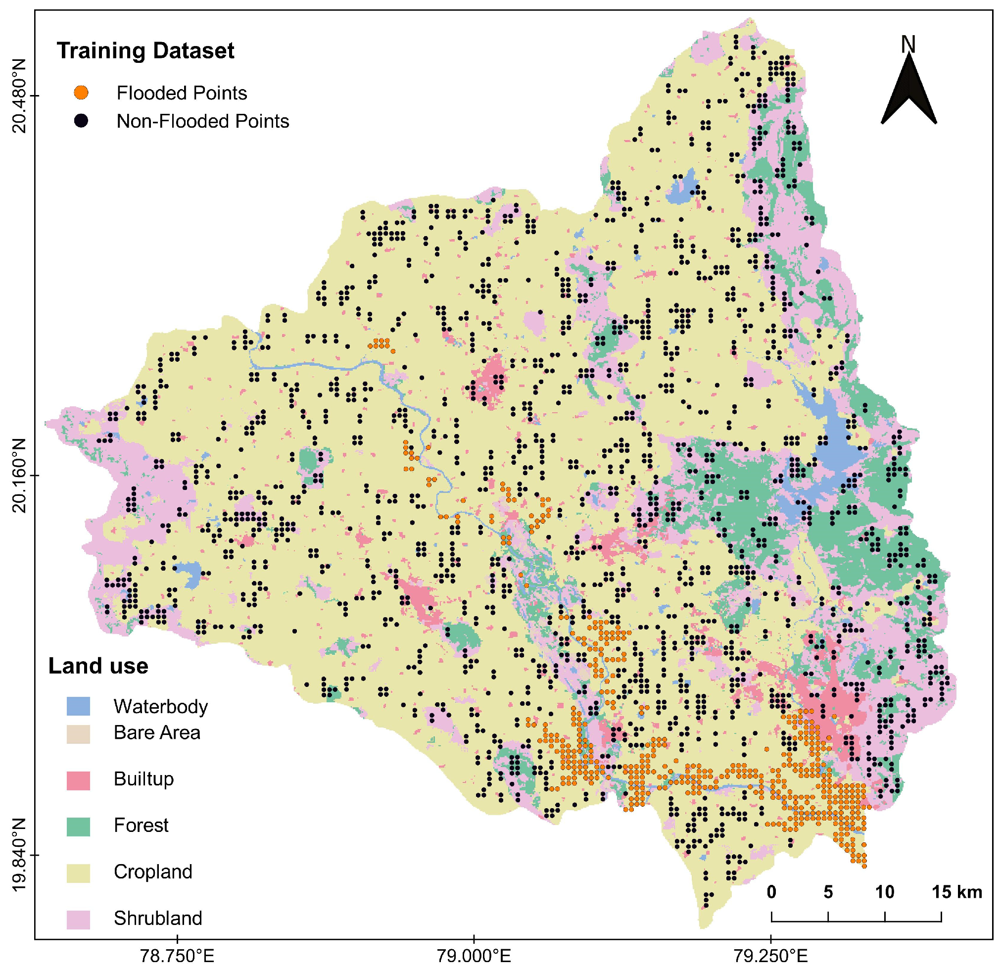
3.2. Flood Inventory Mapping

The collection, preparation, and development of a historical flood database is the backbone of flood hazard studies. Historical flood events were gathered to create a comprehensive flood inventory for the study area. Considering the August 2013 Chandrapur district flood events, which were sourced from the website of the National Remote Sensing Centre [20], the flood inventory map was prepared. The total historical flood event (August 2013 Chandrapur district floods) area covered 76.29 km² (2%) of the study area. The flood inventory dataset had a spatial resolution of 100 m × 100 m; therefore, all flood factors were brought to the same uniform resolution. From the total dataset of 2478 points, a random sample dataset was extracted, encompassing both flooded and non-flooded locations (Figure 2). This random sample dataset was further divided into a training dataset (random 70% of the sample dataset) and a testing dataset (the remaining 30% of the random sample dataset).

3.3. Multi-Collinearity Analysis, Prediction Ability Assessment, and Selection of Factors

A flood is a complex phenomenon, and its genesis depends upon a variety of factors. The causes of floods are generally ambiguous, and hence, flood occurrence is difficult to be associated firmly with a defined number of causative factors. As each region has its own distinct characteristics and features, the flood-contributing factors may vary for different study areas. Optimum selection of flood-contributing factors is difficult as it depends heavily on the complexity of flood occurrence in a particular region [21]. There is no universal convention to be employed for the selection of flood causative factors [22]. In the existing study, the flood-contributing factors were assessed, analyzed, and used for FSM based on a literature review and assessment of geospatial conditions in the study region. The correlation and effectiveness of the selected flood-contributing factors is a prerequisite before developing a model for FSM. Multi-collinearity is a condition where there is a linear relationship or correlation between one or more of the independent variables or inputs. High multi-collinearity in FSM makes it difficult to estimate which factor is really influencing the flood genesis. Hence, if any multi-collinearity issue exists between flood-contributing factors, it should be eliminated. In our study, we have used the variance inflation factor (VIF) method for testing multi-collinearity among flood conditioning variables and the information gain ratio (IGR) method for evaluating the predictive competency of each flood-contributing factor [23]. A tolerance (TOL) score of less than 0.2 and a VIF score of more than 4 signify the existence of multi-collinearity [24]. The average merit (AM) criterion of the IGR method was employed to assess the prominence of each factor in flood prediction. AM = 0 implies the factor has no role in flooding and it should be detached from the modelling process [23]. The VIF and tolerance values of all seven factors analyzed in the study ranged from 1.17 to 2.11 and 0.48 to 0.86, respectively. Hence, it is confirmed that there is no multi-collinearity issue among these conditioning factors. Besides this, the AM values obtained from the IGR method for all the factors ranged from 0.20 to 0.77. It is observed that elevation has a significant influence on flood susceptibility, with an AM score of 0.774, followed by rain (0.739), drainage density (0.562), flow accumulation (0.423), slope (0.233), TWI (0.204) and land use (0.100). None of the factors analyzed have a null value of AM. This proves that they have a significant contribution to the determination of flood susceptibility. Hence, these factors are considered in this study.

3.4. Flood-Contributing Factors

Seven flood-contributing factors viz. elevation, topographic slope, flow accumulation, drainage density, topographic wetness index (TWI), rainfall, and land use were used for FSM in this study. The spatial resolution of these contributing factors was brought to a uniform spatial resolution of 100 m × 100 m (to match with that of the available flood inventory dataset) through resampling in ArcGIS 10.5. The natural break classification method was employed for class division of the factors. Spatial distribution maps for flood-contributing factors were prepared (Figure 3). The relative importance of each factor in FSM and other details associated with class distribution of factors are illustrated below.

• Elevation (m): The height of a geographical feature above mean sea level is termed elevation. Elevation is a key parameter in the determination of flood-susceptible areas, and it also influences the climate of a region. Downstream low-elevation areas are generally more susceptible to flooding. The elevation data were categorized into five classes: (1) 80–110 m, (2) 110–115 m, (3) 115–120 m, (4) 120–125 m, and (5) 125–279 m. The north-eastern and western parts of the study area have elevations more than 220 m. The historical flood data analysis showed that the elevation range of 94–137 m covers almost 70% of the study area and contains the majority of past flood-inundated areas.
• Topographic slope (degree): The slope of a region is the difference between elevations of two points of the region divided by the distance between those two points. Surface runoff and infiltration rates are directly affected by the slope of a region. The slope of the study region was categorized into five classes: (1) 0–1°, (2) 1–2°, (3) 2–3°, (4) 3–4°, and (5) 4–10°. The slope range 0–3° covers nearly 80% of the study area and contains the majority of historical flood events.
• Flow accumulation: Flow accumulation is an indirect method for the determination of drainage areas. In other words, it is an estimation of cells which drain into a given area or cell, and hence acts as a key determinant in flood genesis. Flow accumulation data were categorized into five classes: (1) 0–1 k, (2) 1–5 k, (3) 5–10 k, (4) 10–20 k, and (5) 20–5700 k. The flow accumulation class 0–1 k covers almost half of the study area.
• Drainage density (km/km²): The proportion of the overall length of all the streams and rivers in a drainage basin and the overall area of the drainage basin is termed as drainage density. In other words, it tells us about the capacity of stream networks or rivers to drain out water from the basin or sub-basin. Drainage density was divided into five classes: (1) 0–30 km/km², (2) 30–60 km/km², (3) 60–90 km/ km², (4) 90–120 km/km², and (5) 120–330 km/km². The drainage density in the range 0–80 km/km² covers nearly 80% of the total study area. The drainage density in the range 0–80 km/km² and 150–240 km/km² together cover the majority of historically flooded areas.
• Topographic wetness index (TWI): The TWI is the estimation of the propensity of a region to accrue water. The spatial scale effects on hydrological processes have been studied using the TWI. In other words, it tells us how likely an area is to be wet. The TWI was calculated using the local slope angle and the local ascending area that flows through a certain point per unit contour length. The regions with higher TWI values are expected to be moist in comparison with regions having lesser TWI scores. The TWI was calculated using Equation (1) [25].

  $$\mathrm{TWI}=\ln \left({\displaystyle \frac{{\mathrm{A}}_{\mathrm{s}}}{\mathsf{\theta }}}\right)$$

  (1)

  where ${\mathrm{A}}_{\mathrm{s}}$ is the local ascending area (m²/m) that flows through a certain point per unit contour length, and θ is the local slope angle in degrees. The TWI data were categorized into five classes: (1) 0–7, (2) 7–8, (3) 8–9, (4) 9–10, and (5) 10–14. The TWI range of 6–10 covers about 81% of the study area and the majority of the historical flooded area.
• Rainfall (mm): Rainfall is one of the crucial factors in flooding. The extends of a flood is directly connected to the intensity and duration of rainfall. The rainfall data of the study area from the years 1980 to 2013 were obtained from the Water Resources Department of the Government of Maharashtra [18]. The hourly rainfall data were analyzed using the I-D-F (Intensity–Duration–Frequency) curve method and rainfall depth for the 25-year return period was used for FSM in mm. The rainfall data are categorized into five different classes: (1) 0–90 mm, (2) 90–122 mm, (3) 122–140 mm, (4) 140–160 mm, and (5) 160–200 mm. The rainfall distribution varies from more than 150 mm in the eastern parts to less than 52 mm in the western parts of the study area.
• Land use: Natural as well as human-actuated covering of the earth’s surface represents the land use of an area [7]. Flood frequency is affected by runoff and sediment transport, both of which are influenced by the land use of a region. Land use has an important role in runoff speed, infiltration, and evapotranspiration. By having a direct or indirect influence on many hydrological processes, land use acts as a vital factor for the flood susceptibility study of a region. Land use data were prepared using the Global Land Cover 1992–2019 database at 300 m resolution, available at the European Space Agency Climate Change Initiative website [19]. Land use has been categorized into six classes: (1) waterbody, (2) bare area, (3) built-up region, (4) forest, (5) cropland, and (6) shrubland. The majority of the land use is cropland and it covers 68.84% of the total area, while bare area, which covers only 0.45% of the area of the district, was the least contributing land use class. Water bodies encompass 2.29% of the study area, while built-up regions cover 3.77% of the area. Forest land covers 8.89%, while 15.75% of the area is covered by shrubland.

3.5. Flood Susceptibility Mapping

3.5.1. Frequency Ratio (FR) Model

The interpretation and investigation of relationships between dependent and independent variables are termed as bivariate statistical analysis. The FR model is one of the most extensively used bivariate statistical models for vulnerability forecasting of natural hazards [6]. The principal advantage of the FR model is its simple execution and generation of fully apprehensible outcomes. The significance and worth of each class of particular flood-contributing factors in the FR model were predicted through the calculation of specific model parameters. The higher the weightage of an individual class of particular contributing factor, the greater the role and significance of that class of the factor in flood occurrence prediction. The following weights of the FR model for each flood-contributing factor were estimated (

Table 1. Description of area coverage by flood-contributing factors and parameter values of FR and SEI model for training dataset. Abbreviations used in the table are described in the core content in the corresponding sections.

Flood-Contributing Factors	Subclass	Total Pixel	Total Area (km2)	% of Total Area (X)	Flood Pixel	Flood Area (km2)	% of Flood Area (Y)	FR Model Parameters			SEI Model Parameters
								FR (Y/X)	Relative Frequency (RF)	Prediction Rate (PR)	Pdij	Hj	Hj max	Icj	Pj	Wj
Elevation (m)	80–110	168	1.68	6.78	168	1.68	29.07	4.29	0.32	1.41	0.32	1.94	2.32	0.17	2.65	0.44
	110–115	193	1.93	7.79	187	1.87	32.35	4.15	0.31		0.31
	115–120	188	1.88	7.59	145	1.45	25.09	3.31	0.25		0.25
	120–125	143	1.43	5.77	47	0.47	8.13	1.41	0.11		0.11
	125–279	1786	17.86	72.07	31	0.31	5.36	0.07	0.01		0.01
Slope (degree)	0–1	51	0.51	2.06	27	0.27	4.67	2.27	0.35	1.00	0.35	2.22	2.32	0.04	1.29	0.05
	1–2	1169	11.69	47.18	222	2.22	38.41	0.81	0.13		0.13
	2–3	1048	10.48	42.29	275	2.75	47.58	1.12	0.17		0.17
	3–4	150	1.5	6.05	38	0.38	6.57	1.09	0.17		0.17
	4–10	60	0.6	2.42	16	0.16	2.77	1.14	0.18		0.18
Flow accumulation	0–1 k	2044	20.44	82.49	332	3.32	57.44	0.70	0.07	1.27	0.07	2.10	2.32	0.10	2.13	0.20
	1 k–5 k	143	1.43	5.77	45	0.45	7.79	1.35	0.13		0.13
	5 k–10 k	90	0.9	3.63	34	0.34	5.88	1.62	0.15		0.15
	10 k–20 k	77	0.77	3.11	58	0.58	10.03	3.23	0.30		0.30
	20 k –5700 k	124	1.24	5.00	109	1.09	18.86	3.77	0.35		0.35
Drainage density (km/km2)	0–30	1816	18.16	73.28	147	1.47	25.43	0.35	0.04	1.26	0.04	2.09	2.32	0.10	1.96	0.20
	30–60	342	3.42	13.80	237	2.37	41.00	2.97	0.30		0.30
	60–90	56	0.56	2.26	20	0.2	3.46	1.53	0.16		0.16
	90–120	64	0.64	2.58	27	0.27	4.67	1.81	0.18		0.18
	120–400	200	2	8.07	147	1.47	25.43	3.15	0.32		0.32
TWI	0–7	134	1.34	5.41	27	0.27	4.67	0.86	0.10	1.20	0.10	2.08	2.32	0.10	1.70	0.17
	7–8	1702	17.02	68.68	393	3.93	67.99	0.99	0.12		0.12
	8–9	579	5.79	23.37	116	1.16	20.07	0.86	0.10		0.10
	9–10	36	0.36	1.45	22	0.22	3.81	2.62	0.31		0.31
	10–18	27	0.27	1.09	20	0.2	3.46	3.18	0.37		0.37
Rainfall (mm)	0–90	528	5.28	21.31	45	0.45	7.79	0.37	0.07	1.22	0.07	2.13	2.32	0.08	1.02	0.08
	90–122	393	3.93	15.86	163	1.63	28.20	1.78	0.35		0.35
	122–140	447	4.47	18.04	143	1.43	24.74	1.37	0.27		0.27
	140–160	786	7.86	31.72	182	1.82	31.49	0.99	0.19		0.19
	160–200	324	3.24	13.08	45	0.45	7.79	0.60	0.12		0.12
Land use	Waterbody	4	0.04	0.16	0	0	0.00	0.00	0.00	1.65	0.00	2.04	2.58	0.21	0.87	0.18
	Barren land	9	0.09	0.36	2	0.02	0.35	0.95	0.18		0.18
	Built-up area	99	0.99	4.00	45	0.45	7.79	1.95	0.37		0.37
	Forest land	319	3.19	12.87	88	0.88	15.22	1.18	0.23		0.23
	Cropland	1801	18.01	72.68	437	4.37	75.61	1.04	0.20		0.20
	Shrubland	246	2.46	9.93	6	0.06	1.04	0.10	0.02		0.02

).

• Frequency ratio (FR): The flood incidence and area ratio for each class of contributing factor was first estimated, and thereafter, the FR value of each class was determined. The FR values for each class of a particular flood-contributing factor were computed using Equation (2).

  $${\mathrm{FR}}_{\mathrm{ij}}={\displaystyle \frac{\frac{{\mathrm{P}}_{\mathrm{n}}\left({\mathrm{F}}_{\mathrm{i}\mathrm{j}}\right)}{{\sum }_{\mathrm{i}=1}^{\mathrm{m}}{\mathrm{P}}_{\mathrm{n}}\left({\mathrm{F}}_{\mathrm{i}\mathrm{j}}\right)}\left(\mathrm{f}\mathrm{l}\mathrm{o}\mathrm{o}\mathrm{d}\mathrm{o}\mathrm{c}\mathrm{c}\mathrm{u}\mathrm{r}\mathrm{r}\mathrm{e}\mathrm{n}\mathrm{c}\mathrm{e}\mathrm{r}\mathrm{a}\mathrm{t}\mathrm{i}\mathrm{o}\right)}{\frac{{\mathrm{P}}_{\mathrm{n}}\left({\mathrm{A}}_{\mathrm{i}\mathrm{j}}\right)}{{\sum }_{\mathrm{i}=1}^{\mathrm{m}}{\mathrm{P}}_{\mathrm{n}}\left({\mathrm{A}}_{\mathrm{i}\mathrm{j}}\right)}\left(\mathrm{a}\mathrm{r}\mathrm{e}\mathrm{a}\mathrm{r}\mathrm{a}\mathrm{t}\mathrm{i}\mathrm{o}\right)}}$$

  (2)

  where FR_ij denotes the frequency ratio of class i of factor j; ${\mathrm{P}}_{\mathrm{n}}\left({\mathrm{F}}_{\mathrm{i}\mathrm{j}}\right)$ is the flood pixels in class i of factor j; ${\mathrm{P}}_{\mathrm{n}}\left({\mathrm{A}}_{\mathrm{i}\mathrm{j}}\right)$ is the total area pixels in class i of factor j; m represents the total classes in the particular flood-contributing factor.
  The FR scores for each class of flood-contributing factor can also be calculated by dividing the % of the flooded area enclosed by a particular class of respective factor by the % of the overall study area enclosed by that class.

  $${\mathrm{FR}}_{\mathrm{ij}}={\displaystyle \frac{\mathrm{\%}\mathrm{o}\mathrm{f}\mathrm{f}\mathrm{l}\mathrm{o}\mathrm{o}\mathrm{d}\mathrm{e}\mathrm{d}\mathrm{a}\mathrm{r}\mathrm{e}\mathrm{a}\mathrm{e}\mathrm{n}\mathrm{c}\mathrm{l}\mathrm{o}\mathrm{s}\mathrm{e}\mathrm{d}\mathrm{b}\mathrm{y}\mathrm{p}\mathrm{a}\mathrm{r}\mathrm{t}\mathrm{i}\mathrm{c}\mathrm{u}\mathrm{l}\mathrm{a}\mathrm{r}\mathrm{c}\mathrm{l}\mathrm{a}\mathrm{s}\mathrm{s}\mathrm{o}\mathrm{f}\mathrm{f}\mathrm{a}\mathrm{c}\mathrm{t}\mathrm{o}\mathrm{r}}{\mathrm{\%}\mathrm{o}\mathrm{f}\mathrm{o}\mathrm{v}\mathrm{e}\mathrm{r}\mathrm{a}\mathrm{l}\mathrm{l}\mathrm{s}\mathrm{t}\mathrm{u}\mathrm{d}\mathrm{y}\mathrm{a}\mathrm{r}\mathrm{e}\mathrm{a}\mathrm{e}\mathrm{n}\mathrm{c}\mathrm{l}\mathrm{o}\mathrm{s}\mathrm{e}\mathrm{d}\mathrm{b}\mathrm{y}\mathrm{c}\mathrm{l}\mathrm{a}\mathrm{s}\mathrm{s}}}$$

  (3)

  where FR_ij denotes the frequency ratio of class i of factor j.
• Relative frequency (RF): The relationship between historical flood locations and predictor classes was investigated using relative frequency values. The normalization of previous frequency ratio values as expressed in Equation (4) [10] gives the values of relative frequency.

  $${\mathrm{RF}}_{\mathrm{ij}}={\displaystyle \frac{\mathrm{F}{\mathrm{R}}_{\mathrm{i}\mathrm{j}}}{\sum \mathrm{F}{\mathrm{R}}_{\mathrm{i}\mathrm{j}}}}$$

  (4)

  where RF_ij represents relative frequency value for class i of factor j; FRij stands for the frequency ratio for class i of factor j; $\sum \mathrm{F}{\mathrm{R}}_{\mathrm{i}\mathrm{j}}$ represents the FR total values of all classes of factor j.
• Prediction rate (PR): The interrelationships among the flood-contributing factors were acknowledged through the calculation of prediction rate values. PR values were estimated using Equation (5) [10].

  $${\mathrm{PR}}_{\mathrm{j}}={\displaystyle \frac{{(MaxRF}_j-{MinRF}_j)}{Min({MaxRF}_j-{MinRF}_j)}}$$

  (5)

  where PR_j stands for the prediction rate value of factor j; MaxRFj denotes the uppermost value of RF among all class of factor j; MinRFj represents the smallest value of RF out of all classes of factor j; Min(MaxRF_j − MinRF_j) is the minimum value from all values of (MaxRF_j − MinRF_j) among all factors.

Flood susceptibility mapping using the FR model involves the computation of prediction rate (PR) values for each contributing factor (Table 1). Normalization of the PR values for individual contributing factors yields the FR weights (Equation (6)), with land use (1.65) being distributed equally among the five land use classes before the weights were normalized. Subsequently, the Flood Susceptibility Index (FSI) map for the FR model is generated using Equation (7). This process involved employing the weighted sum option of the spatial analyst tool in ArcGIS 10.5.

FRweights_i = {TWI: 0.133, slope: 0.111, rainfall: 0.135, flow accumulation: 0.141,
    elevation: 0.156, drainage density: 0.139, waterbody: 0.030,
bare area: 0.030, built-up: 0.030, forest: 0.030,   
cropland: 0.030, shrubland: 0.030}          

(6)

$$\begin{array}{cc}\hfill {\mathrm{F}\mathrm{S}\mathrm{I}}_{\mathrm{F}\mathrm{R}}& ={\mathrm{F}\mathrm{R}\mathrm{w}\mathrm{e}\mathrm{i}\mathrm{g}\mathrm{h}\mathrm{t}\mathrm{s}}_{\mathrm{i}}\times \left(\right(1/\mathrm{e}\mathrm{l}\mathrm{e}\mathrm{v}\mathrm{a}\mathrm{t}\mathrm{i}\mathrm{o}\mathrm{n})+\mathrm{f}\mathrm{l}\mathrm{o}\mathrm{w}\mathrm{a}\mathrm{c}\mathrm{c}\mathrm{u}\mathrm{m}\mathrm{u}\mathrm{l}\mathrm{a}\mathrm{t}\mathrm{i}\mathrm{o}\mathrm{n}\hfill \\ & +\mathrm{r}\mathrm{a}\mathrm{i}\mathrm{n}\mathrm{f}\mathrm{a}\mathrm{l}\mathrm{l}+{\sum }_{\mathrm{i}=0}^5{\mathrm{l}\mathrm{a}\mathrm{n}\mathrm{d}\mathrm{u}\mathrm{s}\mathrm{e}}_{\mathrm{i}}+(1/\mathrm{s}\mathrm{l}\mathrm{o}\mathrm{p}\mathrm{e})+\mathrm{d}\mathrm{r}\mathrm{a}\mathrm{i}\mathrm{n}\mathrm{a}\mathrm{g}\mathrm{e}\mathrm{d}\mathrm{e}\mathrm{n}\mathrm{s}\mathrm{i}\mathrm{t}\mathrm{y}+\mathrm{T}\mathrm{W}\mathrm{I}\left)\right)\hfill \end{array}$$

(7)

where

○

FRweights_i represents the normalized weight for ith variable;

○

${\sum }_{\mathrm{i}=0}^5$ denotes the sum across the specified land use attribute.

3.5.2. Shannon Entropy Index (SEI) Model

The entropy of a variable is the “amount of information” contained in the variable. The amount of information is determined not just by the values of the particular variable but also by the amount of surprise that the value of the variable causes. Shannon’s entropy index (SEI) model, which is another bivariate statistical method, provides the basis for a theory around the notion of information by quantifying the amount of information in a variable. The measurement of disorderliness, instability, and uncertainty of a particular system signifies the entropy of the system [8]. Introduced by Claude Shannon in 1948 for the quantification of disorderliness in thermodynamic systems, the entropy model was thereafter used in a variety of studies for measurement of disorderliness in the distribution of values of variables. Greater variability in the spreading of a variable’s values will produce lesser values of entropy and vice versa [7]. The Shannon entropy index (SEI) model has been widely employed in studies for the assessment of natural hazard susceptibility, and through its usage, it can be presumed that the entropy of a flood episode embodies the degree to which various contributing factors impact the incidence of floods [8]. The following SEI model components (Table 1) have been estimated and utilized to decide the flood susceptibility of the study area using the SEI model:

• Probability Density (Pd_ij): Probability density (Pd_ij) was calculated using frequency ratio (FR) values of each class of a particular flood-contributing factor. As expressed in Equation (8), FR values of each class of a particular factor are divided by the sum of FR values of all classes of that factor to obtain the PDij values of each class [8,10]. The probability density (Pd_ij) values of the SEI model correspond to the relative frequency (RF) values of the FR model.

  $$\mathrm{P}{\mathrm{d}}_{\mathrm{i}\mathrm{j}}={\displaystyle \frac{\mathrm{F}{\mathrm{R}}_{\mathrm{i}\mathrm{j}}}{{\sum }_{\mathrm{i}=1}^{{\mathrm{m}}_{\mathrm{j}}}\mathrm{F}{\mathrm{R}}_{\mathrm{i}\mathrm{j}}}}$$

  (8)

  where Pd_ij is the probability density of class i of factor j; FR_ij is the frequency ratio value of class i of factor j; m_j denotes the total classes in factor j.
• Entropy Values (H_j and H_j max): The entropy measurement of each class of a particular factor was carried out using Equations (9) and (10) [7,8].

  $${\mathrm{H}}_{\mathrm{j}}=-\sum _{\mathrm{i}=1}^{{\mathrm{m}}_{\mathrm{j}}}\mathrm{P}{\mathrm{d}}_{\mathrm{i}\mathrm{j}}{\log }_2\mathrm{P}{\mathrm{d}}_{\mathrm{i}\mathrm{j}},\mathrm{j}=1,\dots ,\mathrm{n}$$

  (9)

  $${\mathrm{H}}_{\mathrm{j}\mathrm{m}\mathrm{a}\mathrm{x}}={\log }_2{\mathrm{m}}_{\mathrm{j}}$$

  (10)

  where H_j and H_jmax are the entropy values of factor j; Pd_ij is the probability density of class i of factor j; m_j is the overall classes of a particular flood-contributing factor.
• Information coefficients (Ic_j): Using entropy values, the information coefficient values for each factor have been calculated using Equation (11) [8,10].

  $$\mathrm{I}{\mathrm{c}}_{\mathrm{j}}=\left({\displaystyle \frac{{\mathrm{H}}_{\mathrm{j}\mathrm{m}\mathrm{a}\mathrm{x}}-{\mathrm{H}}_{\mathrm{j}}}{{\mathrm{H}}_{\mathrm{j}\mathrm{m}\mathrm{a}\mathrm{x}}}}\right),\mathrm{j}=1,\dots ,\mathrm{n}$$

  (11)

  where Ic_j is the information coefficient for factor j; H_j and H_jmax represent the entropy values of factor j.
• Weights of factors (W_j): The weight values attributed to each flood-contributing factor were determined using Equation (12) [8].

  W_j = Ic_j × P_j

  (12)

  where W_j is the weight value estimated for factor j; Ic_j is the information coefficient for factor j, and P_j = ${\displaystyle \frac{1}{{\mathrm{m}}_{\mathrm{j}}}}{\sum }_{\mathrm{i}=1}^{\mathrm{m}}\mathrm{F}{\mathrm{R}}_{\mathrm{i}\mathrm{j}}$; FRij is the frequency ratio value of class i of factor j, and mj is the overall classes in factor j.

The execution of flood susceptibility mapping using the SEI model involved calculating the index parameters (Table 1). The weights for this mapping, utilizing the SEI model, were determined through the calculation of entropy and information coefficient values for each flood-contributing factor. The resulting weights (Wj) for each factor were obtained. Like the approach taken in the FR model for flood susceptibility mapping, the weights (Wj) in the SEI model were normalized, and these normalized weights are referred to as SEIweights. Furthermore, land use (0.18) was uniformly distributed among the five land use classes before the weights were normalized. Subsequently, the Flood Susceptibility Index (FSI) map was generated using Equation (14), employing the weighted sum option of the spatial analyst tool in ArcGIS 10.5. This method ensures a comprehensive representation of flood susceptibility, integrating the weighted contributions of each factor, and offers a valuable tool for effective flood risk management.

SEIweights_i = {TWI: 0.128, slope: 0.037, rainfall: 0.060, flow accumulation: 0.151,
    elevation: 0.333, drainage density: 0.151, waterbody: 0.022,
bare area: 0.022, built-up: 0.022, forest: 0.022,  
cropland: 0.022, shrubland: 0.022}         

(13)

$${\mathrm{F}\mathrm{S}\mathrm{I}}_{\mathrm{S}\mathrm{E}\mathrm{I}}={\mathrm{S}\mathrm{E}\mathrm{I}\mathrm{w}\mathrm{e}\mathrm{i}\mathrm{g}\mathrm{h}\mathrm{t}\mathrm{s}}_{\mathrm{i}}\times \left(\begin{array}{c}\left(1/\mathrm{e}\mathrm{l}\mathrm{e}\mathrm{v}\mathrm{a}\mathrm{t}\mathrm{i}\mathrm{o}\mathrm{n}\right)+\mathrm{f}\mathrm{l}\mathrm{o}\mathrm{w}\mathrm{a}\mathrm{c}\mathrm{c}\mathrm{u}\mathrm{m}\mathrm{u}\mathrm{l}\mathrm{a}\mathrm{t}\mathrm{i}\mathrm{o}\mathrm{n}+\mathrm{r}\mathrm{a}\mathrm{i}\mathrm{n}\mathrm{f}\mathrm{a}\mathrm{l}\mathrm{l}\\ +{\sum }_{\mathrm{j}=0}^5{\mathrm{l}\mathrm{a}\mathrm{n}\mathrm{d}\mathrm{u}\mathrm{s}\mathrm{e}}_{\mathrm{j}}+(1/\mathrm{s}\mathrm{l}\mathrm{o}\mathrm{p}\mathrm{e})\times +\mathrm{d}\mathrm{r}\mathrm{a}\mathrm{i}\mathrm{n}\mathrm{a}\mathrm{g}\mathrm{e}\mathrm{d}\mathrm{e}\mathrm{n}\mathrm{s}\mathrm{i}\mathrm{t}\mathrm{y}+\mathrm{T}\mathrm{W}\mathrm{I}\end{array}\right)$$

(14)

where SEIweights_i represents the normalized weight for the ith variable, and ${\sum }_{\mathrm{j}=0}^5{\mathrm{l}\mathrm{a}\mathrm{n}\mathrm{d}\mathrm{u}\mathrm{s}\mathrm{e}}_{\mathrm{j}}$ denotes the sum across the specified land use attribute.

3.6. Performance Evaluation and Validation

3.6.1. Calculation of Statistical Indicators

In this step, the results of the FR and SEI models were statistically analyzed to assess the performance of flood susceptibility mapping [7,8,23]. The testing dataset, representing a random 30% of the sample dataset, was employed for the validation of model outputs. The statistical indicators employed for the performance assessment were as follows:

• Sensitivity: This provides information about the model-computed total number of flood pixels that are accurately categorized as a flood event, and it was calculated as expressed in Equation (15).

  $$\mathrm{Sensitivity}={\displaystyle \frac{\mathrm{T}\mathrm{P}}{\mathrm{T}\mathrm{P}+\mathrm{F}\mathrm{N}}}$$

  (15)

  where TP (true positive) and FN (false negative) are pixels in this study.
• Specificity: This provides information about the model-computed total number of non-flood pixels that are accurately categorized as a non-flood event and was estimated using Equation (16).

  $$\mathrm{Specificity}={\displaystyle \frac{\mathrm{T}\mathrm{N}}{\mathrm{F}\mathrm{P}+\mathrm{T}\mathrm{N}}}$$

  (16)

  where TN (true negative) and FP (false positive) are pixels in this study.
• Accuracy: This provides information on accurately categorized flood pixels and non-flood pixels and was computed using Equation (17).

  $$\mathrm{Accuracy}={\displaystyle \frac{\mathrm{T}\mathrm{P}+\mathrm{T}\mathrm{N}}{\mathrm{T}\mathrm{P}+\mathrm{F}\mathrm{P}+\mathrm{T}\mathrm{N}+\mathrm{F}\mathrm{N}}}$$

  (17)

  where TP (true positive) and TN (true negative) represent pixels that are accurately defined as flooded and non–flooded pixels, and FP (false positive) and FN (false negative) denote the pixels which are inaccurately categorized as flooded and non-flooded.
• Positive prediction value (PPV): This is the likelihood that a flood pixel predicted by the model is an actual flood pixel and was estimated using Equation (18).

  $$\mathrm{PPV}={\displaystyle \frac{\mathrm{T}\mathrm{P}}{\mathrm{T}\mathrm{P}+\mathrm{F}\mathrm{P}}}$$

  (18)
• Negative prediction value (NPV): This is the likelihood that a non-flood pixel predicted by the model is an actual non-flood pixel and was calculated using Equation (19).

  $$\mathrm{NPV}={\displaystyle \frac{\mathrm{T}\mathrm{N}}{\mathrm{T}\mathrm{N}+\mathrm{F}\mathrm{N}}}$$

  (19)

3.6.2. Model Validation Using the AUC-ROC Curve Method

In this step, the results of the FR and SEI models were validated using the area under the receiver-operator characteristic curve (AUC-ROC) method. An ROC curve is created by plotting the sensitivity on the Y-axis against the 1-specificity on the X-axis. The model’s performance can be gauged by the area under the ROC curve, which is a statistical indicator of the model’s success. A competent model is specified by an AUC value adjacent to 1, while an unproductive model is underlined by an AUC value close to 0 (Wang et al., 2021). In AUC-ROC ranges of 0.5–0.6, 0.6–0.7, 0.7–0.8, 0.8–0.9 and 0.9–1, the models are categorized as poor, medium, good, very good and excellent, respectively [23]. The models results were classified and their success rate was computed using the training dataset. The accuracy of the models’ results was decided through the calculation of the prediction rate using the testing dataset. The AUC values can be determined using Equation (20) [10].

$$\mathrm{AUC}={\displaystyle \frac{(\sum \mathrm{T}\mathrm{P}+\sum \mathrm{T}\mathrm{N})}{\mathrm{P}+\mathrm{N}}}$$

(20)

where P stands for overall flood pixels and N represents the entire non-flood pixels.

4. Results

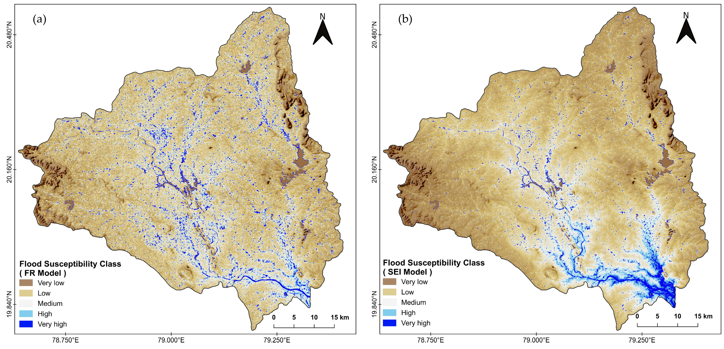
4.1. Frequency Ratio (FR) Model Outcomes

A higher PR value in the FR model signifies a more significant role of that factor in flood susceptibility. Upon evaluation of the PR values, it was established that land use demonstrated the highest PR value at 1.65, followed by elevation (1.41), flow accumulation (1.27), drainage density (1.26), rainfall (1.22), TWI (1.20), and slope (1.00). Notably, the analysis of prediction rates highlights that slope, with a PR value of 1.00, exerts the least influence among the contributing factors. The FR model predicted that 5.4% of the area is under very high flood susceptibility, covering 200 km². The study area exhibited varying levels of susceptibility to flooding, where high susceptibility covers 8.1% (300 km²), moderate 49.6% (1844 km²), low 35.2% (1308 km²), and very low 1.7% (63 km²) of the total area. The flood susceptibility map of the study area constructed using the FR model is shown in Figure 4.

4.2. Shannon Entropy Index (SEI) Model Outcomes

The resulting weights (Wj) for each factor were obtained, with elevation attaining the highest weight (0.44), followed by flow accumulation (0.20), drainage density (0.20), land use (0.18), TWI (0.17), rainfall (0.08), and slope (0.05). Notably, slope, with a weight value of 0.05, emerged as the least contributing factor. The SEI model predicted flood susceptibility as follows: very high (3.8%, 141 km²), high (7.6%, 283 km²), moderate (37.8%, 1404 km²), low (49.1%, 1825 km²), and very low (1.7%, 62 km²). A flood susceptibility map derived from the SEI model is presented in Figure 4.

4.3. Performance Evaluation of Models

In this section, we conduct a performance evaluation of two models, namely the frequency ratio (FR) and Shannon entropy index (SEI), utilizing various statistical indicators (

Table 2. Model performance evaluation using training and testing datasets.

Parameters	FR Model		SEI Model
	Training Dataset	Testing Dataset	Training Dataset	Testing Dataset
True positive (pixels)	162	90	341	184
True negative (pixels)	1330	563	1261	547
False positive (pixels)	2	5	71	21
False negative (pixels)	212	114	33	20
Sensitivity	0.433	0.441	0.912	0.901
Specificity	0.998	0.991	0.946	0.963
PPV	0.987	0.947	0.827	0.897
NPV	0.862	0.831	0.974	0.964
Accuracy	0.874	0.845	0.939	0.946
AUC	0.971	0.966	0.982	0.978
Overall Correlation (R)	0.606	0.580	0.830	0.864
Overall Standard Deviation Ratio (σ)	0.712	0.745	1.034	1.002
Overall Root Mean Square Error (RMSE)	0.354	0.393	0.247	0.230

). The FR model exhibits an accuracy of 0.874 for the training dataset and 0.845 for the testing dataset. In contrast, the SEI model demonstrates superior accuracy, registering 0.939 for training and 0.946 for testing, implying its enhanced capability in predicting flood susceptibility. Key indicators such as sensitivity and specificity highlight the SEI model’s superiority. The higher sensitivity of the SEI model (0.912 in training, 0.901 in testing) compared to the FR model (0.433 in training, 0.441 in testing) indicates its proficiency in identifying true positives.

The success rate and prediction rate of both models were computed (refer to Figure 5 and Table 2). The AUC values for training and testing are 0.97 and 0.96, respectively, in the case of the FR model, while they are 0.98 and 0.97 in the case of the SEI model. The overall correlation, measuring the strength and direction of the linear relationship between observed and predicted values, underscores the SEI model’s superiority. The SEI model exhibited a stronger correlation of 0.830 for training and 0.864 for testing, while the FR model shows a lower correlation in training (0.606) and testing (0.580) (refer to Table 2). The significance of overall correlation (R), overall standard deviation ratio (σ), and overall root mean square error (RMSE) lies in their ability to comprehensively evaluate the model’s performance on both datasets, providing insights into models’ reliability and accuracy in capturing key features. The overall standard deviation ratio (σ), indicating the agreement between predicted and observed value spreads, supports the SEI model’s proficiency, exhibiting a ratio close to 1. Additionally, the overall RMSE assesses the average error magnitude, with lower values in the SEI model indicating superior predictive accuracy. These findings collectively affirm the SEI model’s greater accuracy and reliability in predicting flood susceptibility compared to the FR model.

5. Discussion

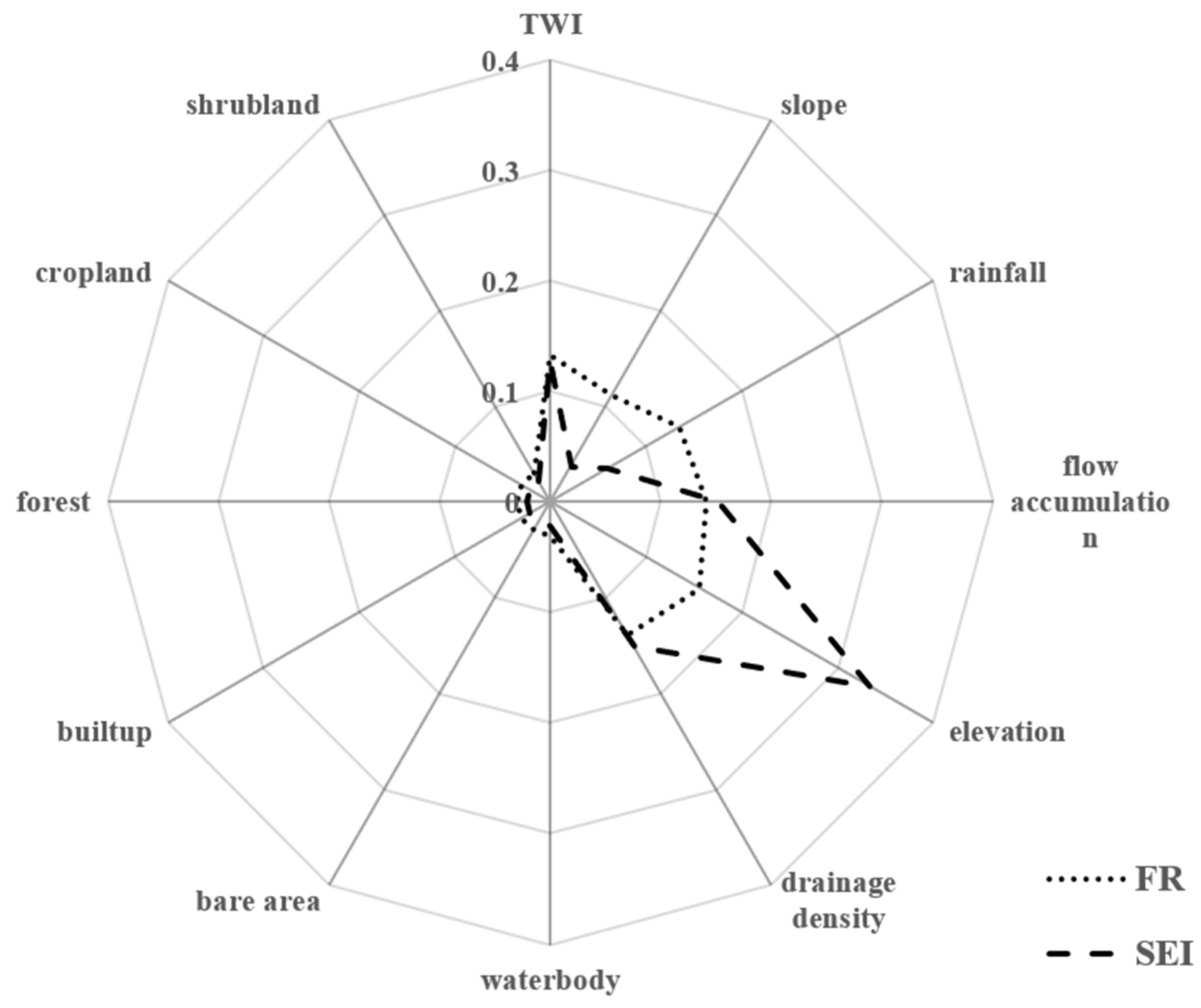
5.1. Analysis of Model Parameters and Their Association with Flood Factors

As per convention, an increase in elevation corresponds to a decrease in FR values, which implies that higher-elevation areas are less susceptible to flooding [11]. As can be seen in Table 1, FR values show a decreasing trend with increases in elevation values. The FR value for the highest elevation range of 125 m–279 m was almost zero. Historical flood data analysis also shows that the first three ranges of elevation (from 80 to 120 m) contain more than 86% of the flooded area. Steeper slopes produce quicker runoff, sending it towards the downslope area. In this study, the highest value of FR corresponds to the lowest slope range. Values of FR greater than one advocate for a greater possibility of flooding [26]. The slope range of 2–3° has an FR value of 1.12, which historically accounts for 47.58% of the flood area. Areas with high flow accumulation values are more prone to flooding as they cannot handle the increased water volume. In this study, increasing values of flow accumulation are followed by increased values of FR. A region with low drainage density will see slower water discharge, which raises the water levels in the channels and causes flooding. Historical flood data showed that the lower drainage density range (30–60 km/km²) with an FR value of 2.97 contains 41% of historical flood areas. Higher values of TWI correspond to more wet and saturated areas. As stated in Section 3.4, regions with higher TWI values are expected to be moist in comparison with regions with lesser TWI scores. As evident from Table 1, the areas falling in highest range of TWI contain the highest value of FR. The rainfall range of 140–160 mm, with an FR value of 0.99, was found to contain the maximum historical flood area. In the case of land use, built-up areas were found to be more susceptible to flooding as they contain the highest (1.95) value of FR. Cropland with an FR value greater than 1 is found to contain more than 75% of flood areas. In a nutshell, the areas with low elevation, low slopes, high flow accumulation, low drainage density, high TWI, and highly urbanized ones are more susceptible to flooding in Chandrapur. A similar trend in FR values for elevation, slope, TWI, and land use is reported by Pawar et al. [11] in their assessment of flood susceptibility for the upper Krishna basin, India. The SEI model also has its basic building blocks in the form of FR values, which in turn are used to compute the probability density (Pd_ij) parameter of the model. Slope, elevation, rainfall, land use, distance to river, topographic wetness index (TWI), and flow accumulation have been reported as the key flood-inducing factors in related flood vulnerability studies [5,10]. The prominent flood-contributing factors found in this study were land use, elevation, flow accumulation, and drainage density. Slope, TWI, and rainfall were the least contributing factors. Sarkar et al. [10] reported a higher significance of rainfall and land use in flood vulnerability assessment pertaining to the urbanized nature of their study region. The lower significance of rainfall and land use as flood affecting agents in the present study can be attributed to the nature of the study area, which is predominantly occupied by cropland and forest. The emergence of flow accumulation and drainage density as key flood-inducing factors also can be linked to the nature of the study region. The crucial role of drainage density in flood induction has been reported by Saha et al. [9] and Sarkar et al. [10]. Flow accumulation has been pronounced as an important factor in FSM in the study by Roopnarine et al. [12].

5.2. Comparing the Model Performance and Weights

Both models provided varying percentage distributions of flood vulnerability zones. The predicted percentage of very-high-flood-risk areas is higher in the FR model (5.4%) than in the SEI model (3.8%). However, the SEI model exhibits superior overall performance in predicting flood susceptibility, characterized by higher accuracy, sensitivity, specificity, correlation, standard deviation ratio, and RMSE. The majority of studies have reported the superior performance of the FR model over the SEI model [8,9,10,12], while the superior performance of the SEI model is reported by Arora et al. [7]. In the current study, the SEI model is judged superior based on its performance in statistical indicators, while on the scale of AUC, both of them performed almost equally. As illustrated in Figure 6, the radar chart serves as a valuable tool for evaluating the weights assigned to various factors influencing flood susceptibility mapping, with values ranging from 0 to 10 indicating their degree of influence. The weights assigned by the FR and SEI models to seven flood-contributing factors considered in the study were investigated. Land use is further categorized into six classes viz. waterbody, forest, bare area, built-up, cropland, and shrubland. Among these 12 factors, both the FR and SEI models highlighted elevation, flow accumulation, drainage density, and land use as pivotal in assessing flood risk. Notably, the FR model assigns lower weights (0.156, 0.141, and 0.139) to elevation, flow accumulation, and drainage density, respectively, while allocating a higher cumulative weight (0.180) to land use. Conversely, the SEI model assigns greater weights (0.333, 0.151, and 0.151) to elevation, flow accumulation, and drainage density, but allocated lower cumulative weight (0.132) to land use. It is crucial to clarify that cumulative weights for land use represent the total weights assigned to various land use classes. These disparities underscore distinct priorities of the models in weighing a factor’s influence on flooding. The FR model emphasized land use, while the SEI model prioritized topographical features such as elevation, in the assessment of flood risk.

5.3. Limitations of the Models and the Contribution of the Study

The current study attempts to simplify the FR and SEI models’ setup process along with their comprehensive assessment. The whole process of comprehending these models revealed some key limitations of such statistical models used for FSM. As the FR and SEI models do not actually simulate the physical flood processes over the catchment, there are certain uncertainties related to the outcomes of these models. Both models heavily rely on historical flood inventory datasets for estimating their parameters and for the validation of the outcomes. Therefore, the accuracy of flood inventories is of paramount importance to evaluate these models. Unavailability or scarcity of past flood records of a region limits the execution of these models. In the absence of an ideal representative sample size, the use of subpar flood inventory datasets leads to imprecise results. Therefore, it is impractical and unreliable to apply statistical models like the FR and SEI models for assessing the flood vulnerability of a region with limited flood data.

Additionally, the calculation of parameters of these models involves a lengthy and cumbersome process. The main goal of the current study was to present a clear procedure for implementing out these models. The assignment of weights, especially for non-range factors (e.g., land use), presents a challenge in bringing uniformity among factors. Giving each subclass of factors a different weight can be achieved through ranking them [12]. It was also discovered during the literature review that there is no precise definition for the computation of final weights that should be used in GIS software to obtain FSMs. The weight calculation procedure is explicatively defined in the current study (Section 3.5), and before the weights of the factors to be used in generating FSMs were normalized, the weight of the land use class supplied by the models was divided equally among its five subclasses. To determine the final weights of factors for FSM, this study suggests an alternative method that involves determining the relationship between flooding and the causative factors through the analysis of model-calculated weights. The suggested approach is employed in this study (Section 3.5) to decide the final expression of slope and elevation factors to decide FSI values, which was based upon the analysis of the relationship of these factors with flooding (Section 5.1).

5.4. Study Limitations and Future Prospects

The use of open-source coarse-resolution data, the small number of factors, the imbalance in parameters of statistical indicators, and the comparatively small flood inventory dataset are the limitations of this study. The execution of models with high-resolution data along with a rich representative sample dataset remains the future scope of this study. Sub-catchment flood vulnerability assessment can also be executed.

6. Conclusions

The FR and SEI statistical models are commonly used for flood vulnerability assessment along with advanced methods using big data and machine learning. The continuous evolution of GIS technology provides new opportunities for better execution of statistical flood susceptibility models. The primary challenge associated with the execution of the FR and SEI models was found to be the complex and ambiguous process of calculating their parameters and weights. With the key objective of the well-defined execution of the above models, the current study assesses flood vulnerability in Chandrapur district, Maharashtra, India. Seven significant flood-contributing factors viz. elevation, topographic slope, flow accumulation, drainage density, topographic wetness index (TWI), rainfall, and land use were used. The performance evaluation of the FR and SEI models was executed, where the SEI model demonstrated slightly superior performance in comparison to the FR model. AUC values of 0.982 for the SEI model and 0.966 for the FR model advocate for their ability to model flood-vulnerable areas. The FR model predicts that 5.4% of the study area is under very high flood susceptibility, while the very highly flood-vulnerable area as forecasted by the SEI model was 3.8% of the study region. The key limitations and uncertainties of these models were highlighted. Several new methods for achieving consistency between the model-provided flood factor weights and the final weights that need to be calculated in order to move forward with FSM is proposed. This study comprehends the entire process of the execution of the FR and SEI models, along with highlighting the key limitations of the models, which provides valuable inputs to the scientific community for better execution of such models. The satisfactory performance of the FR and SEI models in this study underscores their ability to map the flood vulnerability of a region. The flood susceptibility maps and other data provided by this study can assist regional authorities in area planning and disaster management in devising sustainable flood control measures.

References

1. World Economic Forum Global Risks Report 2022. Available online: https://www.weforum.org/publications/global-risks-report-2022/ (accessed on 26 July 2024).
2. Gourley, J.J.; Hong, Y.; Flamig, Z.L.; Arthur, A.; Clark, R.; Calianno, M.; Ruin, I.; Ortel, T.; Wieczorek, M.E.; Kirstetter, P.-E.; et al. A Unified Flash Flood Database across the United States. Bull. Am. Meteorol. Soc. 2013, 94, 799–805. [Google Scholar] [CrossRef]
3. Mrozik, K.D. Problems of Local Flooding in Functional Urban Areas in Poland. Water 2022, 14, 2453. [Google Scholar] [CrossRef]
4. UNDRR Sendai Framework for Disaster Risk Reduction 2015–2030|UNDRR. Available online: http://www.undrr.org/publication/sendai-framework-disaster-risk-reduction-2015-2030 (accessed on 26 July 2024).
5. Kaya, C.M.; Derin, L. Parameters and Methods Used in Flood Susceptibility Mapping: A Review. J. Water Clim. Chang. 2023, 14, 1935–1960. [Google Scholar] [CrossRef]
6. Rahmati, O.; Pourghasemi, H.R.; Zeinivand, H. Flood Susceptibility Mapping Using Frequency Ratio and Weights-of-Evidence Models in the Golastan Province, Iran. Geocarto Int. 2016, 31, 42–70. [Google Scholar] [CrossRef]
7. Arora, A.; Pandey, M.; Siddiqui, M.A.; Hong, H.; Mishra, V.N. Spatial Flood Susceptibility Prediction in Middle Ganga Plain: Comparison of Frequency Ratio and Shannon’s Entropy Models. Geocarto Int. 2021, 36, 2085–2116. [Google Scholar] [CrossRef]
8. Wang, Y.; Fang, Z.; Hong, H.; Costache, R.; Tang, X. Flood Susceptibility Mapping by Integrating Frequency Ratio and Index of Entropy with Multilayer Perceptron and Classification and Regression Tree. J. Environ. Manag. 2021, 289, 112449. [Google Scholar] [CrossRef] [PubMed]
9. Saha, S.; Sarkar, D.; Mondal, P. Efficiency Exploration of Frequency Ratio, Entropy and Weights of Evidence-Information Value Models in Flood Vulnerabilityassessment: A Study of Raiganj Subdivision, Eastern India. Stoch. Environ. Res. Risk Assess. 2022, 36, 1721–1742. [Google Scholar] [CrossRef]
10. Sarkar, D.; Saha, S.; Mondal, P. GIS-Based Frequency Ratio and Shannon’s Entropy Techniques for Flood Vulnerability Assessment in Patna District, Central Bihar, India. Int. J. Environ. Sci. Technol. 2022, 19, 8911–8932. [Google Scholar] [CrossRef]
11. Pawar, U.; Suppawimut, W.; Muttil, N.; Rathnayake, U. A GIS-Based Comparative Analysis of Frequency Ratio and Statistical Index Models for Flood Susceptibility Mapping in the Upper Krishna Basin, India. Water 2022, 14, 3771. [Google Scholar] [CrossRef]
12. Roopnarine, C.; Ramlal, B.; Roopnarine, R. A Comparative Analysis of Weighting Methods in Geospatial Flood Risk Assessment: A Trinidad Case Study. Land 2022, 11, 1649. [Google Scholar] [CrossRef]
13. Megahed, H.A.; Abdo, A.M.; AbdelRahman, M.A.E.; Scopa, A.; Hegazy, M.N. Frequency Ratio Model as Tools for Flood Susceptibility Mapping in Urbanized Areas: A Case Study from Egypt. Appl. Sci. 2023, 13, 9445. [Google Scholar] [CrossRef]
14. District Administration Chandrapur Demography|District Chandrapur, Government of Maharashtra|India. Available online: https://chanda.nic.in/en/demography/ (accessed on 29 July 2024).
15. The Times of India. 350 Rescued as Flood Situation Turns Grim in Chandrapur. Times India, 11 August 2022.
16. Rase, D.M.; Narayanan, P.S.; Mohan, K.N. Impact of Extreme Weather Events in Relation to Floods over Maharashtra in Recent Years. Available online: https://imetsociety.org/wp-content/pdf/vayumandal/2017432/2017432_7.pdf (accessed on 20 August 2024).
17. EORC JAXA Dataset|ALOS@EORC. Available online: https://www.eorc.jaxa.jp/ALOS/index_e.htm (accessed on 31 July 2024).
18. Hydrology Project, Government of Maharashtra Rainfall Data. Available online: https://mahahp.gov.in/DisplayRainfall.aspx?data=Rainfall (accessed on 31 July 2024).
19. ESA Global Land Cover 1992–2019. Available online: https://supply-chain-data-hub-nmcdc.hub.arcgis.com/apps/NMCDC::global-land-cover-1992-2019-1/about (accessed on 31 July 2024).
20. NRSC Bhuvan|ISRO’s Geoportal|Gateway to Indian Earth Observation|Disaster Services. Available online: https://bhuvan-app1.nrsc.gov.in/disaster/disaster.php?id=flood_hz# (accessed on 31 July 2024).
21. Tehrany, M.S.; Pradhan, B.; Jebur, M.N. Flood Susceptibility Mapping Using a Novel Ensemble Weights-of-Evidence and Support Vector Machine Models in GIS. J. Hydrol. 2014, 512, 332–343. [Google Scholar] [CrossRef]
22. Darabi, H.; Choubin, B.; Rahmati, O.; Torabi Haghighi, A.; Pradhan, B.; Kløve, B. Urban Flood Risk Mapping Using the GARP and QUEST Models: A Comparative Study of Machine Learning Techniques. J. Hydrol. 2019, 569, 142–154. [Google Scholar] [CrossRef]
23. Norallahi, M.; Seyed Kaboli, H. Urban Flood Hazard Mapping Using Machine Learning Models: GARP, RF, MaxEnt and NB. Nat. Hazards 2021, 106, 119–137. [Google Scholar] [CrossRef]
24. Bui, D.T.; Ngo, P.-T.T.; Pham, T.D.; Jaafari, A.; Minh, N.Q.; Hoa, P.V.; Samui, P. A Novel Hybrid Approach Based on a Swarm Intelligence Optimized Extreme Learning Machine for Flash Flood Susceptibility Mapping. CATENA 2019, 179, 184–196. [Google Scholar] [CrossRef]
25. Sørensen, R.; Zinko, U.; Seibert, J. On the Calculation of the Topographic Wetness Index: Evaluation of Different Methods Based on Field Observations. Hydrol. Earth Syst. Sci. 2006, 10, 101–112. [Google Scholar] [CrossRef]
26. Shafapour Tehrany, M.; Shabani, F.; Neamah Jebur, M.; Hong, H.; Chen, W.; Xie, X. GIS-Based Spatial Prediction of Flood Prone Areas Using Standalone Frequency Ratio, Logistic Regression, Weight of Evidence and Their Ensemble Techniques. Geomat. Nat. Hazards Risk 2017, 8, 1538–1561. [Google Scholar] [CrossRef]
Figure 1. Study area location map.
Ijgi 13 00297 g001
Figure 2. Training dataset showing flooded and non-flooded points.
Ijgi 13 00297 g002
Figure 3. Spatial distribution maps of flood-contributing factors ((a) elevation; (b) slope; (c) flow accumulation; (d) drainage density; (e) TWI; (f) rainfall; (g) land use).
Ijgi 13 00297 g003
Figure 4. (a) Flood susceptibility map of the study area using the FR model; (b) flood susceptibility map of the study area using the SEI model.
Ijgi 13 00297 g004
Figure 5. (a,c) ROC curves for FR model; (b,d) ROC curves for SEI model.
Ijgi 13 00297 g005
Figure 6. Weights assigned to factors by models demonstrating their role in flooding.
Ijgi 13 00297 g006