Road Network Intelligent Selection Method Based on Heterogeneous Graph Attention Neural Network

Abstract

Selecting road networks in cartographic generalization has consistently posed formidable challenges, driving research toward the application of intelligent models. Despite previous efforts, the accuracy and connectivity preservation in these studies, particularly when dealing with road types of similar sample sizes, still warrant improvement. To address these shortcomings, we introduce a Heterogeneous Graph Attention Network (HAN) for road selection, where the feature masking method is initially utilized to assess the significance of road features. Concentrating on the most relevant features, two meta-paths are introduced within the HAN framework: one for aggregating features of the same road type within the first-order neighborhood, emphasizing local connectivity, and another for extending this aggregation to the second-order neighborhood, capturing a broader spatial context. For a comprehensive evaluation, we use a set of metrics considering both quantitative and qualitative aspects of the road network. On road types with similar sample sizes, the HAN model outperforms other models in both transductive and inductive tasks. Its accuracy (ACC) is higher by 1.62% and 0.67%, and its F1-score is higher by 1.43% and 0.81%, respectively. Additionally, it enhances the overall connectivity of the selected network. In summary, our HAN-based method provides an advanced solution for road network selection, surpassing previous approaches in terms of accuracy and connectivity preservation.

1. Introduction

Cartographic generalization, a fundamental technique in traditional cartography, remains a central focus in the realm of digital cartography, with automatic cartographic generalization standing out as a particularly challenging and innovative research frontier [1,2]. Within the cartographic generalization process, selection serves as the initial and pivotal step. Roads, as essential skeletal elements on maps, not only form a crucial component of maps but also command the attention and interest of both map users and cartographers. Given their significant roles in both social and military contexts, roads have become a focal point of extensive research and practical exploration worldwide, particularly in the realm of automatic road network selection [3,4,5]. Road network selection methods are mainly divided into unsupervised and supervised methods. The road network selection process is essentially a subjective decision made by cartographers based on objective facts, and the use of supervised methods to simulate the decision-making process of cartographic experts is the trend of development at this stage. Since graph neural networks can aggregate neighboring road features to embed their own features better, it is an important research direction to use graph neural networks to simulate the decision-making process of road network selection.

In the process of road network selection, the road type data is extremely important, and there is a wealth of interactive information implied between the road types. Previous studies have treated the road type as a feature in the homogeneous graph, ignoring the interactive information between the road types. Dissimilar homogeneous graphs, heterogeneous graphs, or heterogeneous information networks involve a graph data structure encompassing multiple node types or edge types. The exploration of heterogeneous graphs has gained prominence in graph neural network research, as highlighted by studies [6,7,8,9,10,11,12,13,14,15].

Heterogeneous graph neural networks serve to depict complex heterogeneous objects and their interactions, offering rich semantic information and an effective modeling tool for graph data mining. Leveraging heterogeneous graph neural networks proves advantageous as they can harness the semantic information of roads. The key challenge in using heterogeneous graphs for road network selection lies in designing a method for road node aggregation that aligns with the characteristics of road selection, essentially, the establishment of a meta-path method. This methodological refinement is critical for optimizing the performance of road network selection models.

It is recognized that roads of the same network type are typically designed to fulfill similar traffic demands during the planning and construction phases, serving comparable transportation purposes. For instance, highways are engineered for high-speed traffic, whereas urban arterial roads are constructed to accommodate urban traffic flow. Moreover, planning and design standards exert a pivotal influence on the correlation between different road types. The norms and standards established at the country, regional, or city level significantly shape the planning and design of roads. Similar planning and design standards often result in the creation of similar road types, thereby increasing their correlation. Given this understanding, roads of the same type exhibit the highest correlation. To capture this correlation, two types of meta-paths have been devised based on the principle of road correlation. This principle facilitates the aggregation of the most pertinent road features. Specifically, one is for aggregating features of the same road type within the first-order neighborhood, emphasizing local connectivity, and another extends this aggregation to the second-order neighborhood, capturing a broader spatial context. The rationale behind designing the second type of meta-path is that a single-layer convolution can effectively aggregate features from adjacent road nodes at a greater distance. Leveraging the flexibility provided by the HAN (Heterogeneous graph attention network) model [10], which allows for the manual setting of meta-paths and employs a du-al-layer attention mechanism for embedding road features, the HAN model is employed to embed road features for these two types of meta-paths. This approach enables a more nuanced representation of road characteristics based on their correlation and enhances the capabilities of the road network selection model.

The remainder of this paper is organized as follows. Section 2 briefly reviews studies related to road network selection. Next, Section 3 proposes an automatic road network selection model based on heterogeneous graphical attention neural networks. Then, Section 4 presents experimental data, results, and a detailed analysis of these results. Finally, Section 5 concludes the paper.

2. Related Work

Road network selection encompasses two key aspects: quantity selection and structure preservation. Quantity selection involves determining how many roads should be chosen, while structure preservation focuses on selecting which roads to include. Common methods for quantity selection include the square root model, correlation analysis, regression analysis, the map-suitable area-load method, and the geometric progression method [16]. The square root model and its variants are generally accepted as effective for quantity selection, shifting attention to the challenge of structure preservation. In terms of structure preservation methods, constraint indicators are commonly considered based on semantics, geometry, and topology information. Structure preservation methods can be categorized into unsupervised and supervised approaches.

Unsupervised selection methods include graph theory method [17,18,19,20], block-based methods [21], stroke-based methods [22,23], and road grid density methods [24,25]. These methods primarily focus on the overall morphology of the road network using geometric and topological information. Among them, common improvement methods are based on the stroke-based approach [26]. Some scholars [27] have fused three algorithms (a stroke-based, a grid-based, and a combined stroke-mesh algorithm) with three selection methods and made corresponding improvements. In addition to geometric and topological considerations, road semantic information, such as POI (point of interest), residential areas, and traffic flow data, is also utilized for large-scale urban road network selection based on road functionality [28,29,30,31]. Unsupervised methods generally make better use of spatial and semantic information but require a deep understanding of the interactions between various road information and the formulation of selection rules. However, these methods are less automated because of their high subjectivity in determining constraint indicators and their weights.

The supervised selection methods of road networks have become a focal point of current discussions. With the rapid evolution of artificial intelligence, various techniques, including kernel machine learning [32], BP (backpropagation) neural networks [33], Radial Basis Function [34], decision-tree-based (DT) models [35], and ontology knowledge reasoning [36], have been progressively applied to automate road network selection. Moreover, it has been demonstrated that road networks selected using machine learning models are extremely similar to the atlas maps [37]. Despite these advancements, most supervised selection methods overlook the topological information inherent in road networks. Transforming the road network into a graph structure and employing graph theory in the automatic selection process has gained attention [38,39,40,41].

Leveraging the substantial achievements of deep convolutional neural networks in image recognition, Kipf and Welling [42] extended these networks to graph data, resulting in the development of Graph Convolutional Networks (GCN). While GCN effectively utilizes the topology information, its limited generalization ability, relying on the Laplacian operator, led scholars to introduce attention mechanisms into graph convolution, giving rise to Graph Attention Networks (GAT) [43].

The growing demand for graph convolution operations on large-scale graphs prompted the introduction of Graph Sampling Aggregation Networks (GraphSAGE) [44]. Dissimilar methods aggregate all neighboring nodes, and GraphSAGE samples a subset of road neighboring nodes for aggregation, making it suitable for large-scale graphs. Scholarly studies have found that graph convolutional neural networks can learn spatial relationships [45]. Zhang et al. applied graph convolutional neural networks to automatic road network selection, comparing the performance of three homogeneous graph convolutional networks: GCN, GAT, and GraphSAGE [46]. Addressing the issue of gradient vanishing in deep graph neural networks, Zheng et al. incorporated architectures such as JK-Nets, ResNet, and DenseNet into road network selection, resulting in significant performance improvements [47]. Additionally, Ma et al., Zhu et al., and Guo et al. utilized road stroke data to construct spectral domain graph convolution operators for road network selection [48,49,50]. Some scholars have also applied graph neural networks to the selection of rivers and achieved good results [51,52].

Despite the use of graph neural networks (GNNs) in previous studies for automatic road network selection, several shortcomings persist:

• Not exploring the importance of each feature of graph neural networks in the road network selection task;
• Performance Gaps in Intermediate-Grade Roads: Homogeneous graph selection algorithms exhibit poor performance, particularly concerning intermediate-grade roads. Additionally, there is a need to enhance the overall connectivity of the selected road network;
• Lack of Comparison in Transductive and Inductive Tasks: Previous studies have not adequately compared the selection performance of the model in both transductive and inductive tasks. Transductive tasks involve training a model using road data with a small number of known labels to infer the majority of the remaining labels. Inductive tasks, on the other hand, entail training a model using road data with numerous known labels to predict labels for nodes on a new road dataset. Such comparisons are essential for a comprehensive evaluation of the selection model, especially when considering road au-to-selection tasks in different spatial domains.

Addressing these shortcomings will contribute to the development of more robust and versatile graph neural network models for automatic road network selection.

3. Methods

We recognize the limitations of prior intelligent models in the road network selection task; our proposed approach addresses these shortcomings through a multi-step process. Initially, the dual graph is generated following data processing. Within the framework of a graph neural network, the significance of road features is evaluated using the feature masking method. Subsequently, the HAN model is introduced to refine the road network selection results. This is achieved by strategically designing two types of meta-paths, which capitalize on the road correlation principle. Finally, to validate the effectiveness of our proposed method, comprehensive comparisons are conducted against other classical intelligent models. The assessment encompasses both transductive and inductive tasks in the context of road selection. This rigorous evaluation serves to demonstrate the superiority and versatility of our proposed method in improving the precision and adaptability of road network selection processes. The detailed automatic road network selection process is illustrated in Figure 1.

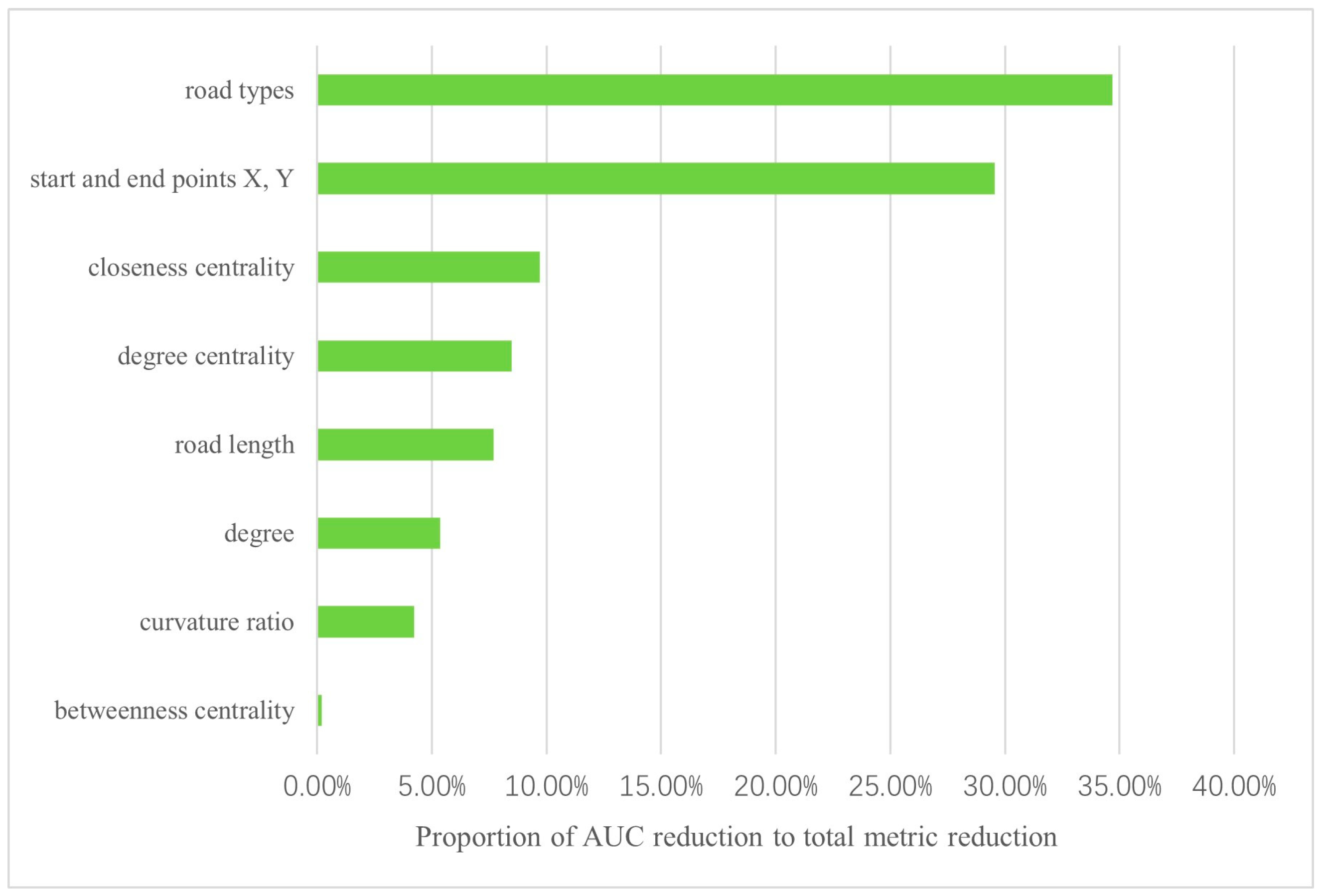
3.1. Measurement of Road Feature Importance Based on Feature Masking Method

During the construction of graph data for road networks, the subjective nature of road feature selection introduces potential issues such as data redundancy, impacting model accuracy. Hence, it is imperative to delve into the significance of different road features in the road selection model. These features primarily stem from three dimensions: geometric, semantic, and topological.

Semantic features encompass road types, while geometric features comprise road length, the number of road vertices, road aspect ratio, mesh density, curvature ratio, and the coordinates of start and end points (X, Y). Topological features include degree, degree centrality, eigenvector centrality, betweenness centrality, and closeness centrality. For detailed information, please consult

Table 1. Road network features.

Feature Types	Feature Indicators	Detailed Explanation
Semantic feature	road type	Road type is a system that classifies roads according to characteristics such as traffic flow, scale, and function.
Geometric features	road length	The length of roads in projected coordinates.
	number of road vertices	The number of vertices in each road polyline.
	road aspect ratio	The ratio of the length of the road’s horizontal coordinates to its vertical coordinates.
	mesh density	The maximum ratio of the perimeter to the area of the left and right polygons associated with each road (if there are no left and right polygons, the value is set to 0).
	curvature ratio	The ratio of the road length to the straight-line length between the start and end coordinates of the road.
	start and end points (X, Y)	Start and end point coordinates (four values in total).
Topological features	degree	The degree of each road is equal to the number of intersections it has with other roads.
	degree centrality	The degree of each road is divided by the total number of roads minus one.
	eigenvector centrality	The eigenvector corresponding to the largest eigenvalue of the adjacency matrix represents the centrality of the eigenvector for each node.
	betweenness centrality	The ratio of the number of times the shortest paths between all other pairs of nodes pass through a particular node to the total number of shortest paths in a graph.
	closeness centrality	The total number of nodes minus one divided by the total number of shortest paths from that node to other nodes.

. Despite the ability of graph neural networks to capture road topology, the consideration of global topological features is currently absent. Consequently, this study also explores the significance of road topological features.

We used a relatively simple feature masking method to assess the importance of road features. Initially, all features slated for evaluation are fed into a two-layer Graph Attention Network (GAT) [43] model for training. The final trained model is determined by selecting the optimal Area Under the Curve (AUC) on the validation set. Subsequently, each feature under scrutiny is individually set to 0, and the ensuing change in the AUC metric on the validation set is observed. The evaluation of road feature importance is contingent upon the observed AUC variation. A higher decrease in the AUC value indicates greater importance for the corresponding road feature.

3.2. Construction of HAN Model for Road Network Selection

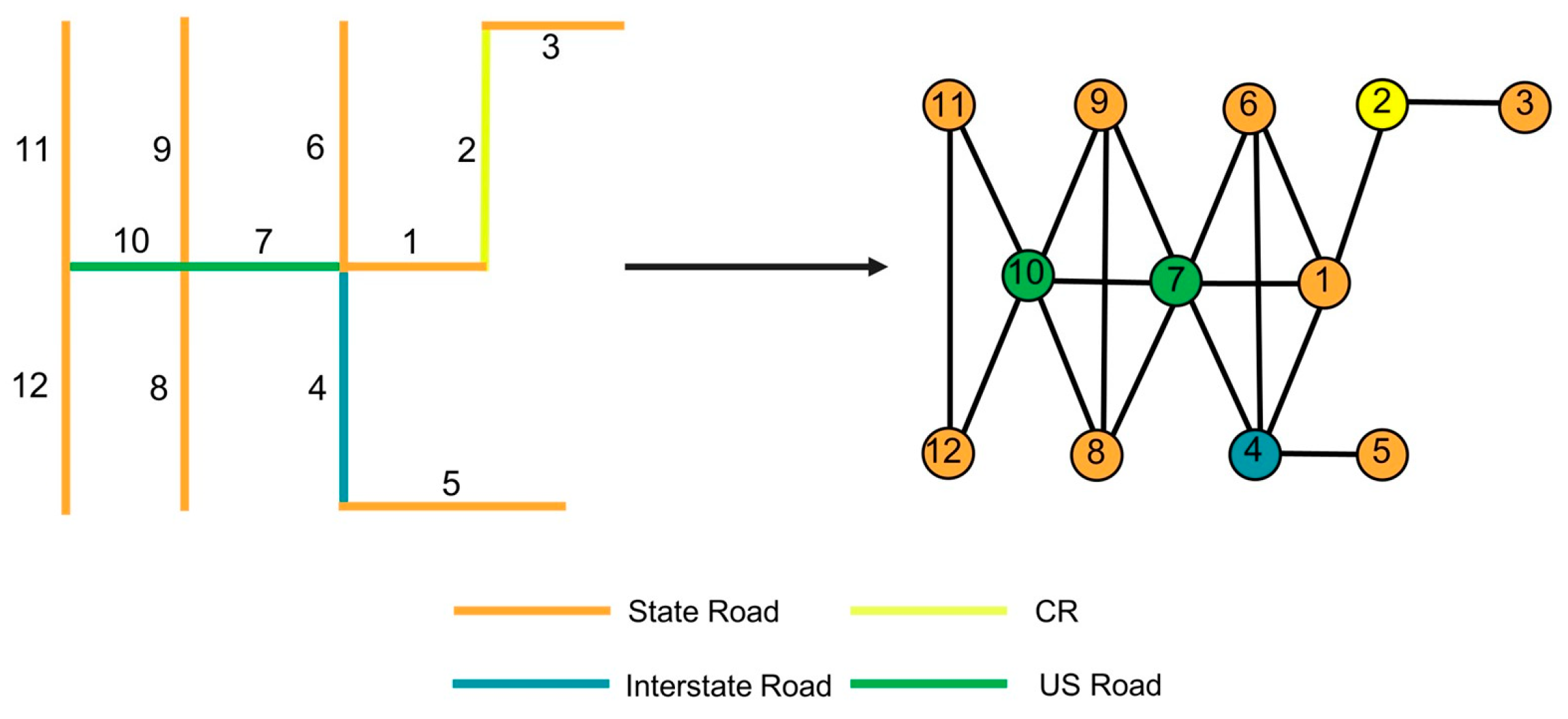
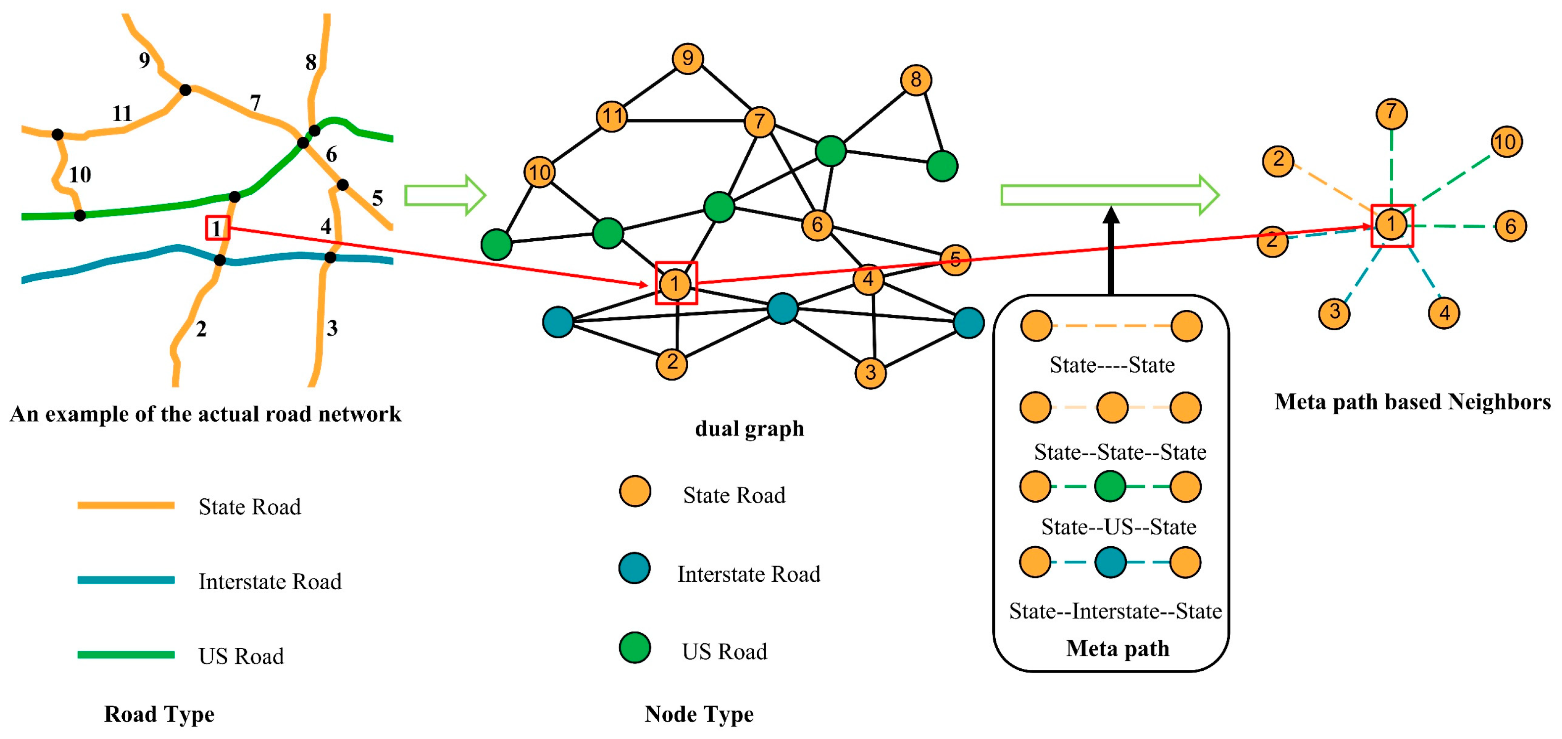
3.2.1. Meta-Path Design Method Based on Road Correlation

Before embarking on meta-path design, it is crucial to establish the methodology for transforming the road network into graph data. In our proposed method, the road network type is designated as the node type in the graph data structure, leveraging the advantages of graph neural networks in embedding node features and aggregating features of neighboring nodes associated with them. In this context, intersections are treated as connecting edges, while roads are construed as nodes within the dual graph. Consequently, the original road network selection transforms into a question of node classification.

Figure 2 illustrates the transformation of a road network into a dual graph, using the U.S. 1M scale road network as an illustrative example. The four road types carry specific meanings:

These distinctions lay the foundation for a nuanced representation of the road network, enabling effective node classification and guiding subsequent meta-path design.

• State Road: Highways constructed and maintained by state governments, facilitating connections between cities and regions within a state.
• US Road: Before the construction of the Highway System, US Roads served as the primary highway network. Nowadays, they continue to play a crucial role as major transportation corridors within states and between regions.
• Interstate Road: The primary objective of an Interstate Road is to enhance the safety and efficiency of automotive travel. Generally, Interstate Roads permit the fastest speeds compared with any other roadways in the vicinity.
• CR: County roads constructed and maintained by local governments serve as vital conduits linking cities and regions within a county.

In the HAN model, the construction of the adjacency matrix deviates from the homogeneous graph convolution algorithm. Specific meta-paths need to be devised for each category of road nodes, enabling the generation of distinct adjacency matrices to capture various semantics. A meta-path, an abstract path pattern delineating node relationships in intricate networks, aids computer models in comprehending network structures. We explain the role of meta-path in terms of road type as shown in Figure 3 below:

Since road segments of the same type often exhibit high correlation, the second-order neighbors belonging to the same road type as a given road segment positively influence its road node embedding. In this study, we utilize first-order neighbor roads as bridges to generate distinct meta-paths. Importantly, meta-paths formed by different types of intermediate bridge roads convey distinct semantic information. For instance, the meta-path ‘State-Interstate-State’ signifies traveling from a State road to an Interstate road and then back to a State road, thus connecting two second-order neighbors of the same road type. Meta-paths enable a deeper comprehension of information flow within intricate networks, thereby enhancing model performance. By searching for semantically connected neighbor nodes, meta-paths facilitate the aggregation of neighboring node features, leading to more effective embeddings of road segment characteristics.

Graph neural networks outperform traditional neural networks in node classification by aggregating neighboring node features to create more robust node embeddings. The core principle involves aggregating node features closely linked to the target node, incorporating the features of neighboring nodes with strong connections. Following this methodology, meta-paths for road networks can be crafted to aggregate features of closely related road nodes.

Given that roads of the same type generally adhere to similar design standards, functions, and purposes, they are inherently more closely related. Consequently, the connectivity and coherence of roads are typically considered during the planning and construction processes.

Two distinct types of meta-paths were formulated for each road type. The first type consolidates node features of the same road type within the first-order neighbors, while the second type encompasses node features of the same road type within the second-order neighbors. In the case of N road types, N + 1 meta-paths are established. In instances where there is no road type attribute, the road network can be hierarchically divided using the back-propagation method based on semantic levels [53]. Subsequently, the corresponding adjacency matrix can be generated following the design principles of meta-paths outlined in the previous section.

Taking the example of roads labeled as ‘State’ in Figure 2, five meta-paths are identified: ① State-State, ② State-State-State, ③ State-US-State, ④ State-Interstate-State, and ⑤ State-CR-State. In summary, two primary categories of meta-paths are developed. The first type aggregates features of the same road type within the first-order neighbors, exemplified by ①. The second type aggregates features of the same road type within the second-order neighbors, illustrated by ②, ③, ④, and ⑤. Consequently, the four road types yield five distinct adjacency matrices. Using the node labeled ‘1’ in Figure 2 as an illustration, the surrounding neighboring nodes aggregated under each meta-path are detailed in

Table 2. The indices of the neighboring nodes that need to be aggregated under each meta-path.

Meta-Path	Indices of Neighboring Nodes to Be Aggregated
State-State	6
State-State-State	none
State-US-State	6, 8, 9
State-Interstate-State	5, 6
State-CR-State	3

.

3.2.2. Heterogeneous Graph Attention Network Embedding Road Features

The Heterogeneous Graph Attention Network is a deep learning model designed to handle heterogeneous graph data characterized by diverse node and edge types. In the context of transforming road networks into graph data, the heterogeneity is manifested in the varied types of roads. Dissimilar to traditional road selection models that typically focus on homogeneous graphs with nodes and edges of the same type, the HAN model autonomously configures meta-paths and employs both node-level and semantic-level attention mechanisms.

Node-level attention refers to the mechanism within a HAN that assigns different weights to neighboring nodes based on their importance to the target node. Given a specific meta-path, a node may have multiple neighbors. Node-level attention aims to distinguish the informative neighbors from the less informative ones by measuring their importance and assigning them corresponding attention weights. In the context of road network embedding, node-level attention determines the aggregation weights when combining the features of neighboring roads under a particular meta-path for each road.

Semantic-level attention, on the other hand, focuses on measuring the importance of different meta-paths. Since different meta-paths can carry different semantic information, it is crucial to determine which meta-paths are more informative for a specific task. Semantic-level attention assigns weights to different meta-paths based on their relevance and importance. In the road embedding scenario, semantic-level attention determines the weight coefficients used in the weighted summation of road embeddings derived from different meta-paths.

To further explain node-level attention and semantic-level attention, Figure 4 shows how the node-level and semantic-level attention mechanisms are aggregated after the road network is transformed into a dual graph.

The HAN model is particularly adept at aggregating road neighboring features under two types of meta-paths. Semantic-level attention in road networks is influenced by road types, leading to varying attention coefficients as road features are embedded and aggregated along different meta-paths. Simultaneously, the node-level attention takes into account the attention weights of different road features from neighboring roads when aggregating features within the same meta-path. The node-level attention [10] coefficient is calculated as:

$${\alpha }_{ij}^{\mathsf{\Phi }}=softma{x}_j\left(e_{ij}^{\mathsf{\Phi }}\right)={\displaystyle \frac{\exp \left(\sigma \left({\mathbf{a}}_{\mathsf{\Phi }}^{\mathrm{T}}\cdot \left[{\mathbf{h}}_i^{\prime }\parallel {\mathbf{h}}_j^{\prime }\right]\right)\right)}{{\sum }_{k\in {\mathcal{N}}_i^{\mathsf{\Phi }}}\exp \left(\sigma \left({\mathbf{a}}_{\mathsf{\Phi }}^{\mathrm{T}}\cdot \left[{\mathbf{h}}_i^{\prime }\parallel {\mathbf{h}}_k^{\prime }\right]\right)\right)}}$$

(1)

where the notation $\parallel$ represents the concatenation operation, ${\mathbf{h}}_i^{\prime }$ and ${\mathbf{h}}_j^{\prime }$ denote the features of its road and the features of the neighboring roads under this meta-path, respectively. Additionally, ${\mathbf{a}}_{\mathsf{\Phi }}$ represents the shared attention weights for the meta-path Φ. The notation $\sigma$ denotes the activation function, and the attention coefficients are normalized through a SoftMax layer.

The semantic-level attention [10] coefficients are calculated as follows:

$$w_{{\mathsf{\Phi }}_p}={\displaystyle \frac{1}{\mid \mathcal{V}\mid }}{\sum }_{i\in \mathcal{V}}{\mathbf{q}}^{\mathrm{T}}\cdot \tanh \left(\mathit{W}\cdot {\mathit{z}}_i^{{\Phi }_p}+\mathit{b}\right)$$

(2)

$${\beta }_{{\mathsf{\Phi }}_p}={\displaystyle \frac{\exp \left(w_{{\mathsf{\Phi }}_p}\right)}{{\sum }_{p=1}^P\mathrm{e}\mathrm{x}\mathrm{p}\left(w_{{\mathsf{\Phi }}_p}\right)}}$$

(3)

$\mathcal{V}$ represents the set of all road nodes, $\mathbf{q}$ is the semantic level attention vector, $\mathit{W}$ is the weight matrix, and $\mathit{b}$ is the bias vector, which are the three trainable parameters shared for all meta-paths. $\mathit{z}$ denotes the node level embedding vector of the ith node under that meta-path. As shown in Equation (3), $w_{{\mathsf{\Phi }}_p}$, which is obtained under all meta-paths, is normalized to obtain the semantic level attention coefficients finally.

In the proposed model, the initial step involves converting the road network into a dual graph. Subsequently, the spatial geometry features, semantic features, and topological features of the roads are amalgamated to construct a feature matrix. In this matrix, each row corresponds to a road, and each column represents a numericalized feature derived from the three types of features. Node-level attention coefficients play a pivotal role in aggregating neighboring road network features for each meta-path, facilitating the generation of node-level embeddings for the road network.

Following this, semantic-level attention coefficients are employed to aggregate the node-level embedding features obtained from each meta-path. This process culminates in the creation of semantic-level embeddings for the road network. It is important to note that the proposed model undergoes training using backpropagation and gradient descent, allowing for iterative refinement of the model parameters to enhance its performance.

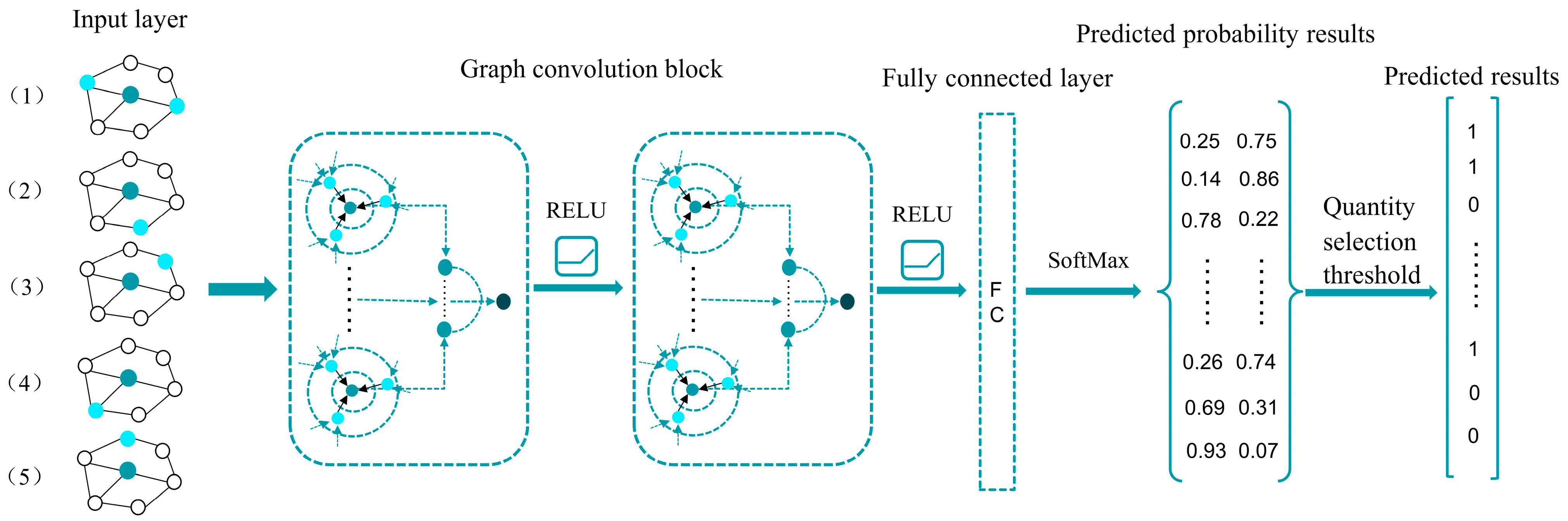
3.3. The Framework of the HAN Model

The framework of the HAN model is depicted in Figure 5. The model is composed of an input layer, a block of graph convolution layers, a fully connected layer, a prediction probability result layer, and a prediction result layer.

Taking the U.S. 1 M scale road network as an example, the input layer represents five adjacency node graphs denoted by (1)–(5), each requiring aggregation under five distinct meta-paths. The HAN model’s graph convolution module primarily involves aggregating node-level features using computed node-level attention coefficients and semantic-level features using semantic-level attention coefficients. The graph convolution block comprises two convolution layers, utilizing the ReLU function as a non-linear activation function and applying Dropout for regularization.

The fully connected layer compresses the feature matrix into a prediction result matrix of size CR*RR. CR refers to the row number of the matrix, indicating a specific road for prediction purposes, while RR represents the number of columns in the matrix, which corresponds to the respective probabilities of selecting or not selecting a particular road. The prediction probability result layer indicates the likelihood of selecting or not selecting each road segment. The prediction result layer determines the selection status of a road segment based on a selection threshold, where 1 indicates selection and 0 indicates non-selection.

The model is trained using the backpropagation gradient descent algorithm, with cross-entropy loss serving as the training objective and the Adam optimizer employed for the training process.

3.4. Evaluation Metrics for the HAN Model

The assessment of road network selection quality is primarily centered on validating the preservation of spatial distribution characteristics, ensuring an appropriate density, and scrutinizing potential disruptions to road connectivity, among other considerations. Spatial distribution characteristics encapsulate the overall features of the road network, providing a comprehensive overview of its structure and layout. In contrast, density characteristics emphasize local attributes, focusing on the density and compactness of roadways within specific areas. Preserving these characteristics necessitates subjective qualitative evaluation, enabling a thorough understanding of the road network’s layout and functionality.

The evaluation of road network selection results in this paper predominantly encompasses quantitative metrics and an assessment of spatial distribution. The AUC, ACC, and f1-score indicators serve as the primary metrics for evaluating the quantitative aspects of road network selection results. The AUC metric identifies the optimal model from the validation set, while the ACC and f1-score metrics gauge the model’s proficiency in automatically selecting road networks. Furthermore, the evaluation includes road network density, as well as the number of isolated roads and their total length, to appraise the spatial distribution quality of the selection result.

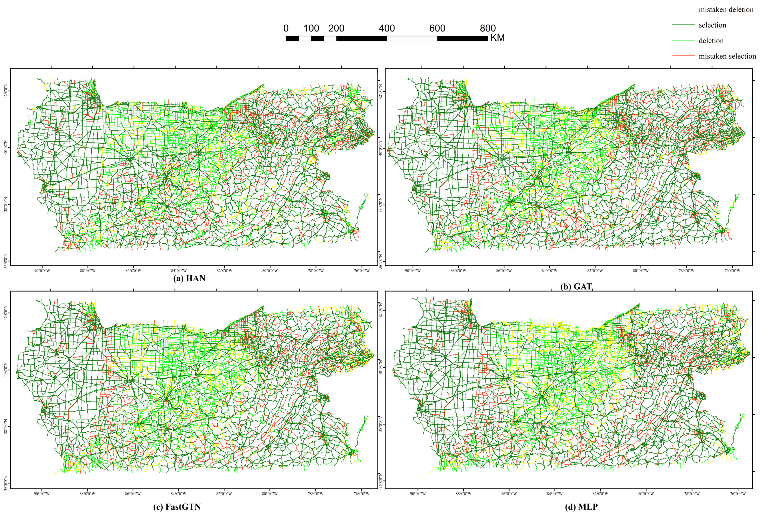
3.4.1. Evaluation Metrics for Quantity Assessment of the HAN Model

AUC, ACC, and f1-score stand as widely employed evaluation metrics for binary classification models. ACC signifies the proportion of correctly predicted labels to the total number of samples. The ACC value serves as an indicator of the model’s quality. Its calculation formula is expressed as follows [47]:

$$ACC={\displaystyle \frac{TP+TN}{TP+FP+FN+TN}}$$

(4)

where True Positive (TP) denotes the instances where both predicted and true values are positive, indicating true positive cases and False Positive (FP) represents instances where the predicted value is positive while the true value is negative, indicating false positive cases. False Negative (FN) signifies instances where the predicted value is negative while the true value is positive, indicating false negative cases. True Negative (TN) denotes instances where both predicted and true values are negative, indicating true negative cases.

The calculation principle of AUC involves determining the area under the Receiver Operating Characteristic (ROC) curve. This curve is formed by adjusting the probability threshold from 0 to 1, with the False Positive Rate (FPR) on the X-axis and the True Positive Rate (TPR) on the Y-axis. The calculation formulas are as follows [47]:

$$FPR={\displaystyle \frac{FP}{FP+TN}}TPR={\displaystyle \frac{TP}{TP+FN}}$$

(5)

Furthermore, given the imbalanced distribution of positive and negative labels in road network data, AUC is employed as the evaluation metric for the road selection model on the validation set.

The f1-score, as the harmonic mean of recall and precision, provides an assessment of the model’s performance on positive samples. In this study, the f1-score is utilized to evaluate the model’s performance, specifically on positive samples. The formula for calculating the f1-score is expressed as [47]:

$$f1\_score={\displaystyle \frac{2Precision\ast Recall}{Precision\ast Recall}}$$

(6)

The calculation formulas for recall and precision are defined as follows:

$$Precision={\displaystyle \frac{TP}{TP+FP}}Recall={\displaystyle \frac{TP}{TP+FN}}$$

(7)

3.4.2. Road Network Density

Road network density is characterized as the ratio of the total length of roads within a specific area to the total area of that region, providing a measure of road density within the designated area. The calculation for road network density is described by [47] as:

$$\rho ={\displaystyle \frac{L_{sum}}{S}}$$

(8)

where $L_{sum}$ represents the sum of the lengths of all roads within the specific area, $S$ represents the area of a specific region. In this study, the road network density is selected as an evaluation metric for the model to assess its performance. The primary objective is to compare the road network density chosen by experts with that of the automatically selected road model.

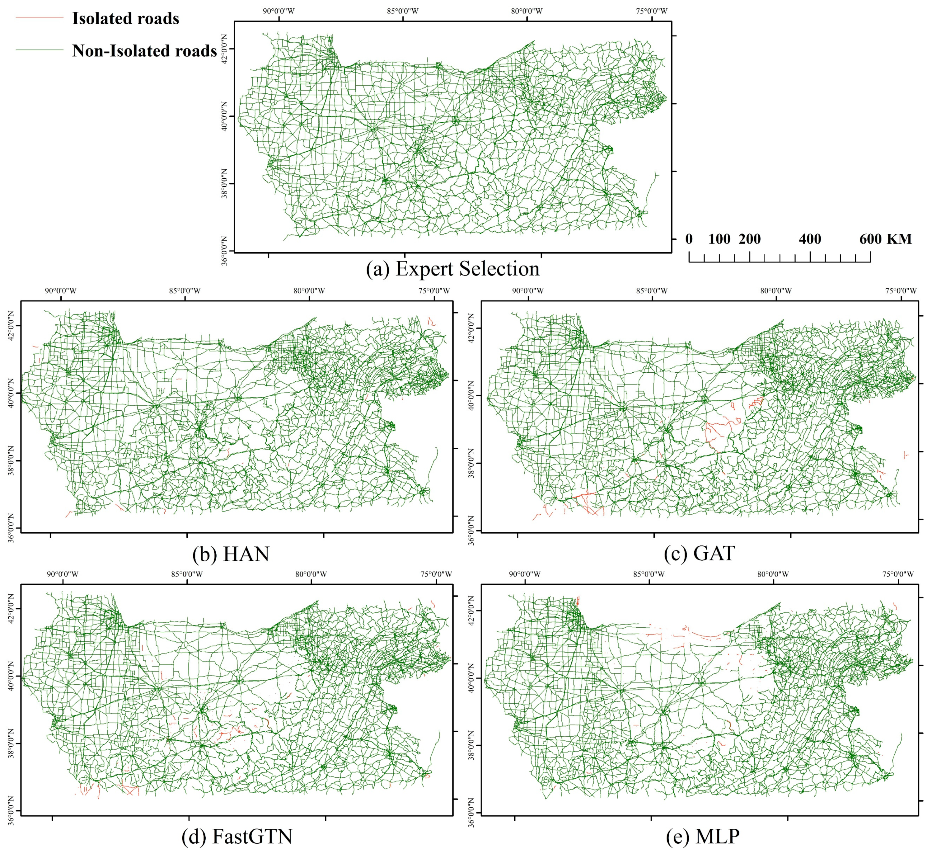
3.4.3. Metrics Related to Isolated Road

To assess the connectivity of the chosen road network, both the total number and length of isolated roads are taken into account. The following method is employed to derive these metrics: Initially, the road network selected by the automatic selection model is transformed into graph data, focusing on road intersections. Subsequently, the largest connected subgraph within these graph data is extracted. Finally, roads within this largest connected subgraph lacking road intersections are identified as isolated roads. UtilizingArcGIS 10.2, the total length and count of isolated roads are computed. Lower values for the total length and number of isolated roads indicate enhanced connectivity of the selected roads.

4. Experimental Process and Results

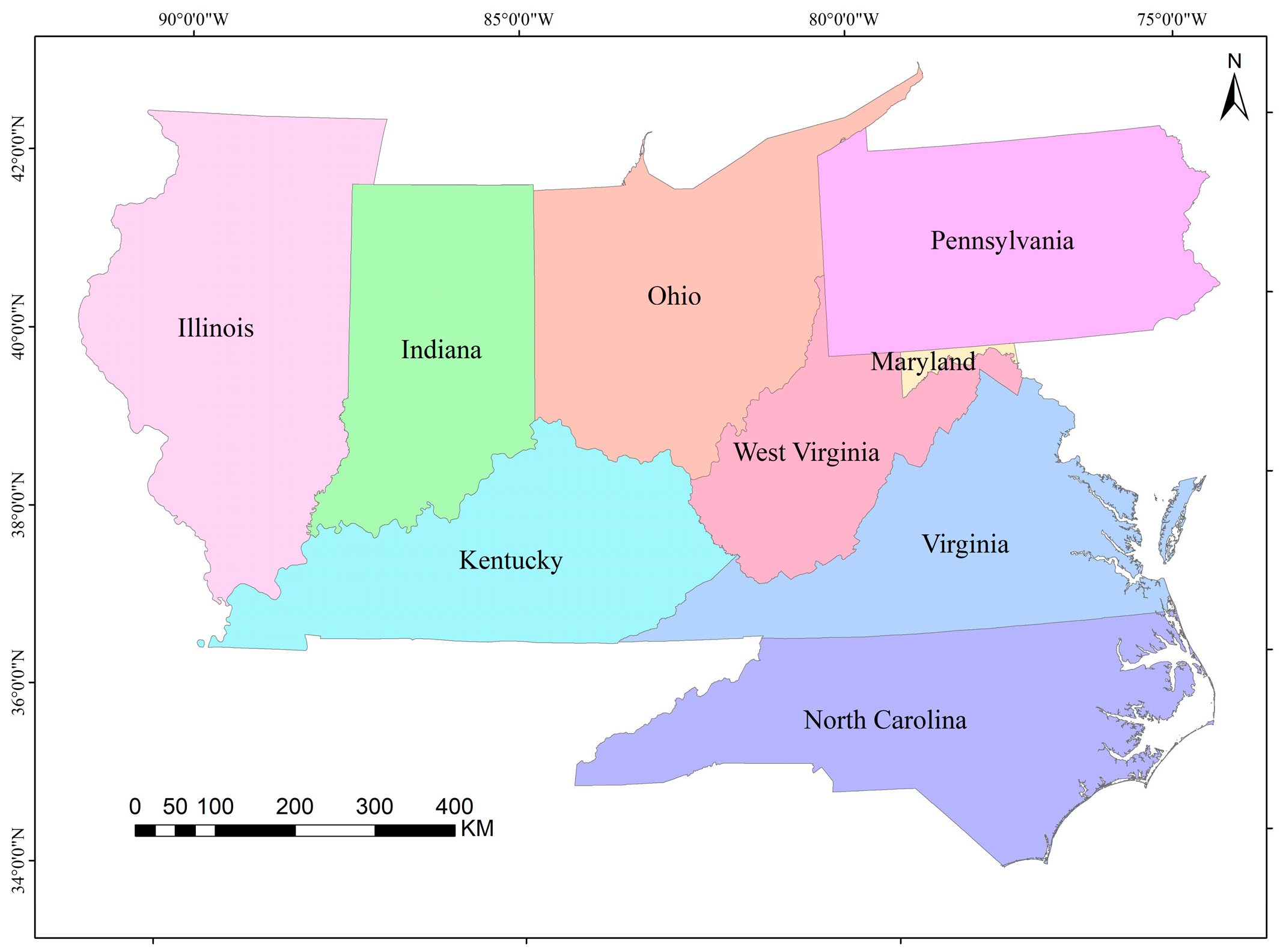
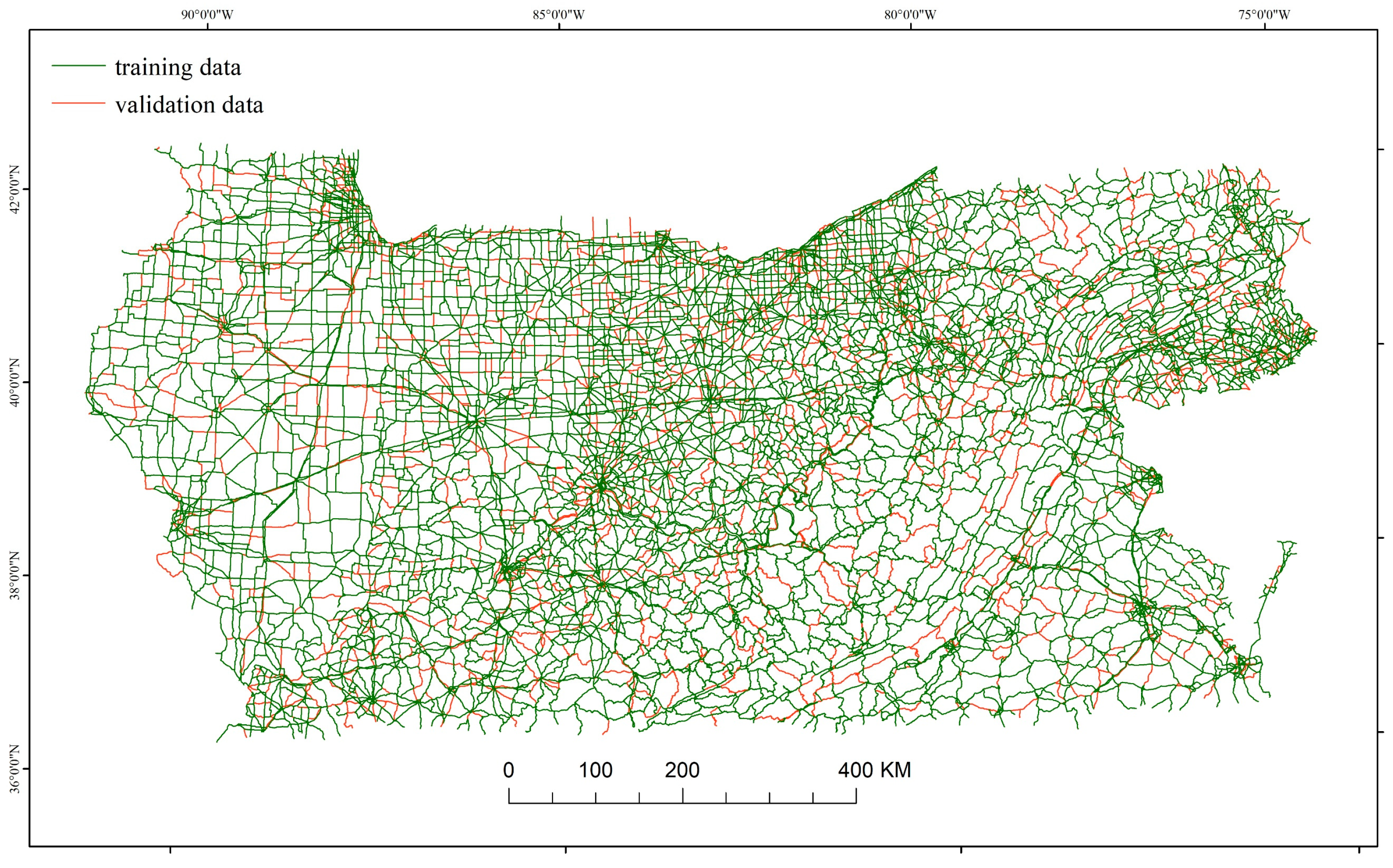
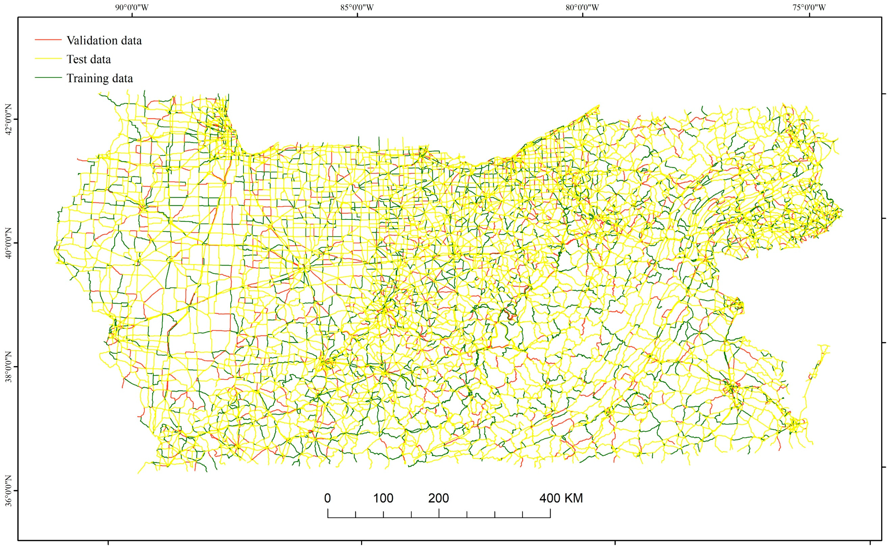
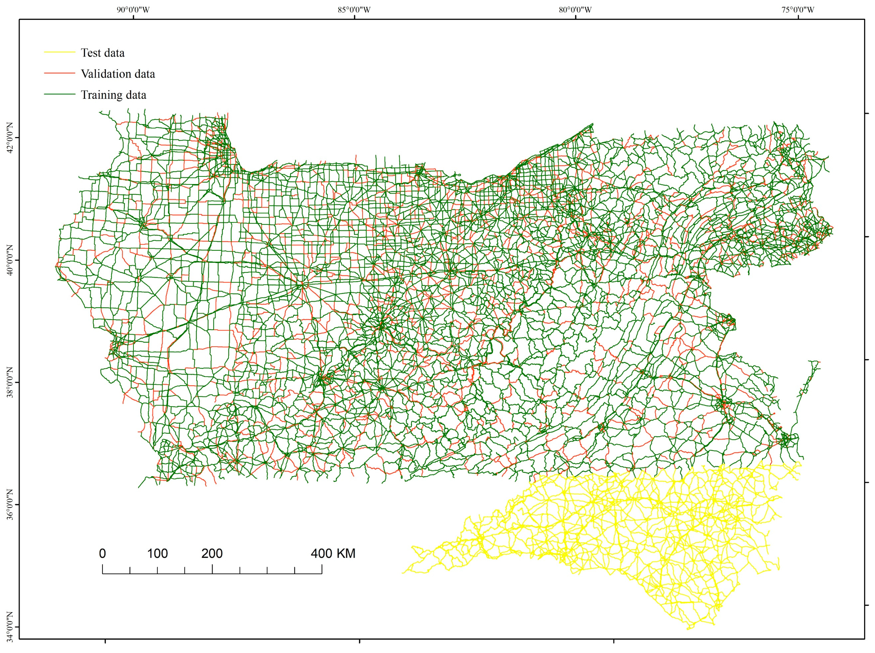
4.1. Experimental Data and Data Preprocessing

Experimental data in this study comprise road network data of the United States, sourced from the USGS and encompassing both 1 M and 2 M scale datasets. The experimental area chosen for analysis consists of nine eastern states of the United States, characterized by intricate road networks. These states include Illinois, Indiana, Kentucky, Ohio, West Virginia, Virginia, Pennsylvania, North Carolina, and parts of Maryland, as illustrated in Figure 6. The road network at scales of 1 M and 2 M within the study area is visualized in Figure 7.

To investigate the significance of road features, this study employed data from the first seven states and portions of Maryland. Employing an 8:2 ratio, positive and negative samples of various road types were randomly stratified and divided into training and validation sets. The count of positive and negative samples for each road type is presented in

Table 3. Quantitative statistics of road data for feature importance exploration.

Road Types	Positive Training Samples	Negative Training Samples	Positive Validation Samples	Negative Validation Samples	Total
State	4840	4151	1221	1042	11,254
US	4205	266	1030	63	5564
Inter	1861	64	471	15	2411
CR	14	18	7	4	43

, while the spatial distribution of the two datasets is visualized in Figure 8.

For the transductive road selection task, the division of training, validation, and testing sets was performed through stratified random sampling of positive and negative samples in a ratio of 2:1:7. The spatial distribution of these three datasets is illustrated in Figure 9, and the corresponding quantitative statistics are presented in

Table 4. Quantitative statistics of road data for the transductive road network selection model.

Road Types	Positive Training Samples	Negative Training Samples	Positive Validation Samples	Negative Validation Samples	Positive Testing Samples	Negative Testing Samples	Total
State	1205	1037	607	518	4249	3638	11,254
US	1061	64	517	34	3657	231	5564
Inter	462	20	241	9	1629	50	2411
CR	1	3	1	2	19	17	43

.

For the inductive road network selection model, the training and validation sets consist of positive and negative samples divided using stratified random sampling in an 8:2 ratio. The testing set is exclusively from North Carolina. The spatial distribution of the three datasets is depicted in Figure 10, and the quantity distribution is outlined in

Table 5. Quantitative statistics of road data for the inductive road network selection model.

Road Types	Positive Training Samples	Negative Training Samples	Positive Validation Samples	Negative Validation Samples	Positive Testing Samples	Negative Testing Samples	Total
State	4869	4162	1192	1031	495	702	12,451
US	4165	255	1070	74	1095	133	6792
Inter	1864	63	468	16	268	46	2725
CR	21	18	0	4	0	1	44

.

Data preprocessing encompasses the removal of isolated road segments and the execution of topological construction. For 1 M road types, missing road types are imputed based on the road types connected to them in 2 M road data. Label construction for these training data primarily involves generating buffers at two different scales and then assigning labels based on the coverage area ratio of these buffers. Road network data slated for selection are assigned a label attribute of 1, indicating positive samples, while the remaining road network data receive a label attribute of 0, denoting negative samples. Following manual verification and adjustment of data labels, intersecting lines are segmented. Subsequently, the geometric and topological features of each road segment are computed, and ultimately, adjacency and feature matrices are constructed.

4.2. Results of Road Feature Importance Measurement

To assess the significance of road features in the divided dataset, a two-layer Graph Attention Network (GAT) road network auto-extraction model is employed, aligning with the framework of the HAN model. In the construction of the feature matrix for the GAT model, road types are encoded using one-hot encoding. Initially, all features are fed into the GAT model, featuring a hidden layer with 64 neurons, 4 attention heads, and a dropout rate of 0.1. The training steps and weight decay coefficient are manually adjusted. The model undergoes training for 1000 epochs, and the model exhibiting the highest AUC on the validation set is chosen as the final benchmark model, achieving an optimal AUC of 0.8413. Subsequently, the evaluated features are set to 0 in the feature matrix, and the trained model is employed to observe the change in AUC, thus gauging the contribution of each feature to the model. The experimental results are presented in

Table 6. The statistical results of AUC on the validation set are based on the feature masking method.

Road Types	Road Length	Mesh Density	Number of Road Vertices	Road Aspect Ratio	Curvature Ratio
0.6108	0.7902	0.8414	0.8417	0.8413	0.8131
Betweenness Centrality	Eigenvector Centrality	Closeness Centrality	Start and End Points X, Y	Degree	Degree Centrality
0.8399	0.8414	0.7767	0.6449	0.8056	0.7850

.

The AUC changes in road features that positively impact the GAT model are consolidated, and the proportion of each feature in the total sum is calculated. The results are visually represented in Figure 11.

The results indicate that road type holds the highest importance, followed by start and end points (X, Y), closeness centrality, degree centrality, road length, degree, curvature ratio, and betweenness centrality.

Table 7. Accuracy of various road types in the GAT validation set.

Road Type	State Road	US Road	Interstate Road	CR
ACC	0.6681	0.9424	0.9691	0.7273

showcases the selection outcomes of the GAT model on the validation dataset, utilizing the partition threshold established by the total count selected by experts.

The GAT model exhibits insufficient performance for the State and CR road types, with limited discussion on the CR road type due to its constrained data volume. Particularly for the State Road type, characterized by a relatively balanced distribution of positive and negative samples, the GAT model’s performance falls short of expectations. Consequently, there arises a need to develop dedicated automatic selection models tailored to specific road types within the road network. In response, the HAN model is introduced for the automatic selection of roads, enabling classification-based selection. The subsequent automatic road network selection model selects start and end points X, Y, closeness centrality, degree centrality, road length, degree, and curvature ratio as features for model training.

4.3. Analysis of the Results of the Transductive and Inductive Road Network Selection Task

To evaluate the selection performance of the HAN model, it is compared with three other models: the Multi-layer Perceptron (MLP), the homogeneous graph neural network GAT, and the Fast Graph Transformer Networks (FastGTN) [14]. The MLP model serves as a baseline without graph convolution, enabling us to assess the impact of graph convolutions on performance. The GAT model incorporates graph convolution but without meta-path aggregation, helping us understand the effect of this aggregation on road network selection. Last, the FastGTN model generates all meta-paths of arbitrary length, allowing for a comparison to derive performance differences between arbitrarily generated meta-paths and our designed meta-paths.

4.3.1. Analysis of the Road Selection Results in the Transductive Task

The transductive task involves training a model on these same graph data with a small number of known labels to infer the majority of the remaining labels. This task requires the model to generalize beyond the training samples, especially when dealing with limited labeled data. The application of this task to road selection occurs when only a few road segments are known, and the objective is to predict the selection of the remaining road segments within the same road network.

The parameters for the various models are configured as follows: The MLP model features 512 hidden layers, while both the HAN and GAT models have hidden layers with 64 neurons, 4 attention heads, and a dropout rate of 0.1. Conversely, the FastGTN model is characterized by hidden layer neurons set to 128 with 4 channels. In the FastGTN model, the initial matrix considers the adjacency of all road types, resulting in a total of N^2 initial matrices, where each road type is adjacent to N other road types.

The weight decay coefficients and training step lengths are manually adjusted, and the training process is conducted for 1000 epochs. The final model is selected based on the optimal AUC on the validation set, which is suitable for imbalanced binary classification problems, and performance metrics are compared on the test set. Since the model output represents selection probabilities when aggregated from 1 M to 2 M, the threshold for the selection quantity is determined based on road data of two different scales.

The HAN model selects roads based on road types individually, and all models in this study use expert-selected quantities for various road types to establish selection thresholds. Given the limited quantity of CR-type roads, the HAN model cannot be adequately trained for this specific road type. Consequently, individual comparisons for CR roads are not conducted, and the overall selection results for CR roads in the HAN model are computed based on the GAT model’s selection results. To standardize variables, CR-type roads in other models are also based on the GAT model’s selection results.

In these experimental road network data, the number of positive and negative samples for state roads is relatively balanced.

Table 8. The statistical results of road selection models in the transductive task.

Evaluation Metrics	Model	All	State	US	Interstate
ACC	HAN	0.7535	0.6416	0.9051	0.9363
	GAT	0.7385	0.6163	0.8976	0.9517
	FastGTN	0.7433	0.6254	0.8968	0.9488
	MLP	0.7316	0.6120	0.8876	0.9398
f1 score for positive samples	HAN	0.8257	0.6664	0.9495	0.9671
	GAT	0.8152	0.6440	0.9455	0.9751
	FastGTN	0.8156	0.6521	0.9451	0.9735
	MLP	0.8104	0.6395	0.9402	0.9710
Isolated roads (number|total length)	HAN	40|343.01 km	26|278.57 km	4|9.80 km	10|54.64 km
	GAT	198|1757.45 km	61|712.64 km	130|998.95 km	7|45.87 km
	FastGTN	281|1342.01 km	243|990.96 km	38|351.06 km	0|0 km
	MLP	245|942.37 km	104|362.05 km	80|338.94 km	61|241.37 km
Road network density (km/km2)	Expert Selection	0.13513	0.06675	0.04855	0.01961
	HAN	0.14212	0.07309	0.04912	0.01938
	GAT	0.14591	0.07721	0.04845	0.01973
	FastGTN	0.13784	0.0682	0.04934	0.01971
	MLP	0.13661	0.0692	0.04746	0.01939

illustrates that the HAN model’s selection for State-type roads surpasses other models in terms of ACC and f1-score. Specifically, ACC and f1-score are 1.62% and 1.43% higher, respectively, compared with the other models. Overall, for the selection by the HAN model, ACC and f1-score are 1.02% and 1.01% higher, respectively, than other models. In terms of the quantity and total length of isolated roads, the HAN model records 158 fewer roads and 1414.44 km less than other optimal models.

The comparison of the selection results of the four models with the expert selection results is depicted in Figure 12. The four models tend to under-select the middle of the road network, although the HAN model and the GAT model show improvement. Additionally, the HAN model exhibits the lowest number of isolated roads among the four models. The main reason why most of the isolated roads appear at the edges of the road network is because the cropping operation of the road network destroys the original topological features of the roads at the margins, so it produces many isolated roads appearing at the margins of the road network.

To assess the spatial equilibrium of road network density, this study partitions the road network into 5 km grids aligned with the study area. The standard deviation of road network density across these grids is computed to determine the evenness of the selected road density distribution. The experts’ selected 5 km grid exhibits a road network density standard deviation of 0.059187, whereas the HAN model exhibits a standard deviation of 0.069638, the GAT model has a standard deviation of 0.069483, the FastGTN model has a standard deviation of 0.069356, and the MLP model exhibits a standard deviation of 0.073987.

To examine the spatial distribution of selection and deletion outcomes from selection models, Figure 13 compares the spatial distribution of the selection results from the four models with the expert selection results. Notably, all four selection models exhibit a significant number of erroneous deletions in the central region of the road network and a notable number of erroneous selections in the upper right corner.

4.3.2. Analysis of the Road Selection Results in the Inductive Task

The inductive task involves training a model on a graph dataset with numerous known labels to predict the labels of nodes in a new graph. This task is particularly suitable for road auto-selection tasks in different spatial domains. The parameters for different models are configured as follows: The HAN model features 512 hidden layers, 4 attentional heads, and a dropout rate of 0.1, while the GAT model has 64 hidden layers, 4 attentional heads, and a dropout rate of 0.1. On the other hand, the MLP has 512 hidden layers, and the FastGTN has 512 hidden layers and 4 channels. The training step size and weight decay rate are manually adjusted. A total of 1000 epochs are trained, and the model with the highest AUC on the validation set is selected as the final model for testing on the test set. Due to the limited number of CR road types, they were not analyzed separately.

Table 9. The statistical results of road selection models in the inductive task.

Evaluation Metrics	Model	All	State	US	Interstate
ACC	HAN	0.7021	0.5589	0.8306	0.7452
	GAT	0.7011	0.5522	0.8225	0.7962
	FastGTN	0.6904	0.5322	0.8339	0.7325
	MLP	0.6608	0.5038	0.7964	0.7093
F1 score for positive samples.	HAN	0.7804	0.4667	0.9050	0.8507
	GAT	0.7799	0.4586	0.9004	0.8806
	FastGTN	0.7710	0.4343	0.9068	0.8582
	MLP	0.7519	0.4000	0.8932	0.8545
Isolated roads (number|total length)	HAN	18|77.62 km	3|11.91 km	15|65.72 km	0|0 km
	GAT	89|695.19 km	40|320.10 km	48|374.08 km	1|1.02 km
	FastGTN	37|443.38 km	10|189.37 km	27|254.02 km	0|0 km
	MLP	72|242.31 km	2|2.36 km	52|191.15 km	18|48.80 km
Road network density (km/km2)	Expert Selection	0.10662	0.03395	0.06002	0.01266
	HAN	0.11179	0.03924	0.06015	0.01361
	GAT	0.11228	0.03991	0.05938	0.01299
	FastGTN	0.11916	0.04468	0.06118	0.01330
	MLP	0.09833	0.03250	0.05368	0.01215

indicates that the HAN model outperforms other models in selecting State-type roads, achieving higher accuracy (ACC) and f1-score. Specifically, the HAN model surpasses other optimal models by 0.67% and 0.81% in terms of ACC and f1-score, respectively. In terms of the quantity and total length of isolated roads, the HAN model falls short of other optimal models, with 19 fewer roads and 365.76 KM less than other models.

The comparison of the selection results of the four models with the expert selection results is depicted in Figure 14. The spatial distribution of the road network selected by the MLP model is highly dispersed, with large voids in the middle. This occurs because the MLP cannot aggregate information from neighboring nodes to update its nodes, such as a graph neural network. Consequently, a certain amount of topological neighborhood information is neglected during model training, resulting in a poor spatial distribution of the selected results. Numerous isolated roads are present in both the FastGTN and GAT models. Overall, the HAN model performs better than the other models, exhibiting the minimum number of isolated roads. The density standard deviation of the 5 km grid selected by the experts is 0.06117, while that of the HAN model is 0.058875, the GAT model is 0.059803, the FastGTN model is 0.06099, and the MLP model is 0.072805.

To examine the spatial distribution of the selection and deletion results of the four models, Figure 15 compares their selection outcomes with the expert’s selection. The comparison reveals that the MLP model exhibits numerous mistakenly deleted roads concentrated in the middle of the road network, while the FastGTN model shows more mistaken selections in the road network. In contrast, the HAN and GAT models display more evenly distributed patterns of mistakenly deleted roads. These findings suggest that the HAN and GAT models exhibit more balanced and consistent selection results compared with the other models.

4.3.3. Analysis of Ablation Study Results

To gain a deeper understanding of the advantages of aggregating neighboring road features based on the meta-paths we designed, we analyzed the results of the two types of experiments from an ablation perspective. For the transductive task, as depicted in Table 8, when compared with the results obtained from our designed meta-path selection (HAN model selection), removing this meta-path selection (GAT selection) led to an increase of 158 isolated roads and a total length increase of 1414.44 km. Substituting it with the results from aggregating road neighbor node features using meta-paths of arbitrary lengths and types (FastGTN) resulted in an increase of 241 isolated roads and a total length increase of 999.0 km. Similarly, for the inductive task, as shown in Table 9, removing the meta-path selection (GAT selection) caused an increase of 71 isolated roads and a total length increase of 617.57 km. Substituting it with the results from aggregating road neighbor node features using meta-paths of arbitrary lengths and types (FastGTN) led to an increase of 37 isolated roads and a total length increase of 365.76 km. These findings demonstrate that aggregating neighboring road features according to the meta-paths we designed can enhance the connectivity of the selection results.

4.4. Exploring Selection Performance at Various Scales and in Various Locations

To investigate the selection performance of the HAN road network automatic selection model across different regions and scales, this paper utilizes the 1:250,000 road network data of Hebi City, China, as the foundational test dataset. Subsequently, the 1:1,000,000 road network data is selected through the application of the HAN road network selection model. Given that the road network data used in this study exhibits incomplete semantic features pertaining to road levels, this paper employs a back-propagation method based on semantic levels [53] to classify the road network levels. Furthermore, the square root model is utilized to determine the sequence of selections, proceeding from higher to lower levels. Thereafter, the HAN Road Network Automatic Selection Model is employed to select roads at a scale of 1:1,000,000, specifically targeting a particular type of road that was not fully selected previously. This process yields the selection probability of each road segment, which is ultimately divided by a threshold. The selection outcomes are presented in Figure 16, demonstrating the preservation of the spatial distribution and connectivity of the road network. These results indicate that the HAN road network automatic selection model exhibits robust performance in selecting road networks of various scales and across different regions.

5. Conclusions and Discussion

Our objective is to tackle the challenges encountered by homogeneous graph neural networks in accurately selecting road types within a road network, especially when dealing with similar numbers of selections and deletions. Additionally, we aim to enhance the spatial distribution of the selected road network. To achieve this, we have devised two distinct meta-paths for each road type, adhering to the principle of aggregating the most pertinent features from neighboring nodes. This approach allows us to construct a heterogeneous graph attention network specifically designed for intelligent road network selection.

In addition, we have applied the feature masking method to explore the significance of three key road features in automatic road network selection models based on graph neural networks: geometric features, semantic features, and topological features. Our findings uncover that road type stands out as the most crucial feature, closely followed by start and end points (X, Y), closeness centrality, degree centrality, length, degree, curvature ratio, and betweenness centrality. However, the effects of mesh density, the number of road vertices, and eigenvector centrality on the automatic road network selection task of graph neural networks are slight.

For the transductive road network selection task, the HAN model demonstrates superior performance compared with the other optimal models. It achieves a 1.62% higher accuracy and a 1.43% higher F1-score in the selection and deletion of a similar number of State Road types. When considering the overall selection results, the HAN model further outperforms the remaining optimal models by increasing accuracy metrics and F1-Score by 1.02% and 1.01%, respectively. Additionally, the HAN model significantly reduces the number of isolated road networks and the total length of the selection results by 79.78% and 63.60%, respectively, compared with the other models.

In the inductive road network selection task, the HAN model also excels, achieving a 0.67% higher accuracy index and a 0.81% higher F1-Score than the remaining optimal models for State Road types. Furthermore, the HAN model reduces the number and length of isolated road networks by 51.35% and 67.96%, respectively, compared with the other models. This improved performance can be attributed to the second-layer convolution of the HAN model, which effectively extracts a wider range of peripheral node features, as four out of its five mating paths are second-order neighbors.

It is worth emphasizing that while FastGTN can indeed automatically generate a range of meta-paths, it falls short in effectively incorporating the background knowledge specific to road network selection. Experimental results underscore the superiority of the HAN model presented in this article, which is explicitly designed based on road correlation. When compared with the FastGTN model, the HAN model demonstrates superior efficiency and accuracy in road network selection tasks. This advantage can be attributed to the HAN model’s ability to leverage domain-specific knowledge, enabling it to make more informed and precise decisions during the selection process.

The primary contribution of this paper lies in quantifying the significance of road features within graph neural network models, a set of evaluation metrics used to assess the road network selection results, and innovatively designing two distinct meta-paths for road network aggregation based on neighboring node features. By applying a heterogeneous graph neural network to the automated selection of road networks, we have established individual, automated selection models tailored for each road type.

Across two road network selection tasks, our approach enhances the precision of selecting road types with a comparable number of deletions and significantly mitigates the issue of excessively isolated roads within the selected network. Notably, our current research has not delved into the model’s performance for road network selection using existing methods to generate road types in scenarios where road type attributes are absent.

Future work will focus on exploring which methods generate road types that yield optimal performance within this model. Additionally, since this paper’s training utilized road network data of a single scale, our future exploration will delve into the enhancement of road network selection performance through joint training across multiple scales., thus broadening its applicability and further validating its utility in real-world scenarios.

References

1. Li, Z.; Liu, W.; Xu, Z.; Ti, P.; Gao, P.; Yan, C.; Lin, Y.; Li, R.; Liu, C. Cartographic Representation of Spatio-Temporal Data: Fundamental Issues and Research Progress. Acta Geod. Cartogr. Sin. 2021, 50, 1033. [Google Scholar]
2. Wang, J.; Wu, F.; Yan, H. Cartography: Its Past, Present and Future. Acta Geod. Et Cartogr. Sin. 2022, 51, 829. [Google Scholar]
3. Reichstein, M.; Camps-Valls, G.; Stevens, B.; Jung, M.; Denzler, J.; Carvalhais, N.; Prabhat. Deep Learning and Process Understanding for Data-Driven Earth System Science. Nature 2019, 566, 195–204. [Google Scholar] [CrossRef]
4. Kronenfeld, B.J.; Buttenfield, B.P.; Stanislawski, L.V. Map Generalization for the Future: Editorial Comments on the Special Issue. ISPRS Int. J. Geo-Inf. 2020, 9, 468. [Google Scholar] [CrossRef]
5. Li, Z.; Lan, T.; Ti, P.; Xu, Z. Advances in Cartography from the Perspective of Maslow’s Hierarchy of Needs. Acta Geod. Cartogr. Sin. 2022, 51, 1536. [Google Scholar]
6. Sun, Y.; Han, J. Mining Heterogeneous Information Networks: A Structural Analysis Approach. SIGKDD Explor. Newsl. 2013, 14, 20–28. [Google Scholar] [CrossRef]
7. Zhang, J.; Lu, C.T.; Zhou, M.; Xie, S.; Chang, Y.; Yu, P.S. Heer: Heterogeneous Graph Embedding for Emerging Relation Detection from News. In Proceedings of the 2016 IEEE International Conference on Big Data (Big Data), Washington, DC, USA, 5–8 December 2016. [Google Scholar]
8. Dong, Y.; Chawla, N.V.; Swami, A. Metapath2vec: Scalable Representation Learning for Heterogeneous Networks. In Proceedings of the 23rd ACM SIGKDD International Conference on Knowledge Discovery and Data Mining, Halifax, NS, Canada, 13–17 August 2017; Association for Computing Machinery: New York, NY, USA, 2017; pp. 135–144. [Google Scholar]
9. Sankar, A.; Zhang, X.; Chang, K.C.C. Meta-Gnn: Metagraph Neural Network for Semi-Supervised Learning in Attributed Heterogeneous Information Networks. In Proceedings of the 2019 IEEE/ACM International Conference on Advances in Social Networks Analysis and Mining (ASONAM), Vancouver, BC, Canada, 27–30 August 2019. [Google Scholar]
10. Wang, X.; Ji, H.; Shi, C.; Wang, B.; Ye, Y.; Cui, P.; Yu, P.S. Heterogeneous Graph Attention Network. In Proceedings of the World Wide Web Conference 2019, Online, 13–17 May 2019. [Google Scholar]
11. Yun, S.; Jeong, M.; Kim, R.; Kang, J.; Kim, H.J. Graph Transformer Networks. In Advances in Neural Information Processing Systems; MIT Press: Cambridge, MA, USA, 2019. [Google Scholar]
12. Zhou, S.; Bu, J.; Wang, X.; Chen, J.; Hu, B.; Chen, D.; Wang, C. Hahe: Hierarchical Attentive Heterogeneous Information Network Embedding. arXiv 2019, arXiv:1902.01475. [Google Scholar]
13. Jia, X.; Dong, Y.; Zhu, F.; Qian, J. Research Progress of Heterogeneous Graph Convolutional Networks. Comput. Eng. Appl. 2021, 57, 36–49. [Google Scholar]
14. Yun, S.; Jeong, M.; Yoo, S.; Lee, S.; Yi, S.S.; Kim, R.; Kang, J.; Kim, H.J. Graph Transformer Networks: Learning Meta-Path Graphs to Improve Gnns. Neural Netw. 2022, 153, 104–119. [Google Scholar] [CrossRef]
15. Bing, R.; Yuan, G.; Zhu, M.; Meng, F.; Ma, H.; Qiao, S. Heterogeneous Graph Neural Networks Analysis: A Survey of Techniques, Evaluations and Applications. Artif. Intell. Rev. 2023, 56, 8003–8042. [Google Scholar] [CrossRef]
16. Wu, F.; Gong, X.; Du, J. Overview of the Research Progress in Automated Map Generalization. Acta Geod. Cartogr. Sin. 2017, 46, 1645–1664. [Google Scholar]
17. Jiang, B.; Claramunt, C. A Structural Approach to the Model Generalization of an Urban Street Network*. GeoInformatica 2004, 8, 157–171. [Google Scholar] [CrossRef]
18. Touya, G. A Road Network Selection Process Based on Data Enrichment and Structure Detection. Trans. GIS 2010, 14, 595–614. [Google Scholar] [CrossRef]
19. Weiss, R.; Weibel, R. Road Network Selection for Small-Scale Maps Using an Improved Centrality-Based Algorithm. J. Spat. Inf. Sci. 2014, 9, 71–99. [Google Scholar] [CrossRef]
20. Shoman, W.; Gülgen, F. Centrality-Based Hierarchy for Street Network Generalization in Multi-Resolution Maps. Geocarto Int. 2016, 32, 1352–1366. [Google Scholar] [CrossRef]
21. Gülgen, F.; Gökgöz, T. A Block-Based Selection Method for Road Network Generalization. Int. J. Digit. Earth 2011, 4, 133–153. [Google Scholar] [CrossRef]
22. Thomson, R.C. The Stroke’ Concept in Geographic Network Generalization and Analysis. In Progress in Spatial Data Handling: 12th International Symposium on Spatial Data Handling; Riedl, A., Kainz, W., Elmes, G.A., Eds.; Springer: Berlin/Heidelberg, Germany, 2006; pp. 681–697. [Google Scholar]
23. Zhou, Q.; Li, Z. A Comparative Study of Various Strategies to Concatenate Road Segments into Strokes for Map Generalization. Int. J. Geogr. Inf. Sci. 2012, 26, 691–715. [Google Scholar] [CrossRef]
24. Chen, J.; Hu, Y.; Li, Z.; Zhao, R.; Meng, L. Selective Omission of Road Features Based on Mesh Density for Automatic Map Generalization. Int. J. Geogr. Inf. Sci. 2009, 23, 1013–1032. [Google Scholar] [CrossRef]
25. Zhou, Q.; Li, Z. Empirical Determination of Geometric Parameters for Selective Omission in a Road Network. Int. J. Geogr. Inf. Sci. 2015, 30, 263–299. [Google Scholar] [CrossRef]
26. Liu, Y.; Li, W. A New Algorithms of Stroke Generation Considering Geometric and Structural Properties of Road Network. ISPRS Int. J. Geo-Inf. 2019, 8, 304. [Google Scholar] [CrossRef]
27. Benz, S.A.; Weibel, R. Road Network Selection for Medium Scales Using an Extended Stroke-Mesh Combination Algorithm. Cartogr. Geogr. Inf. Sci. 2014, 41, 323–339. [Google Scholar] [CrossRef]
28. Xu, Z.; Wang, Z.; Yan, H.; Wu, F.; Duan, X.; Sun, L. A Method for Automatic Road Selection Combined with Poi Data. J. Geo-Inf. Sci. 2018, 20, 159–166. [Google Scholar]
29. Deng, M.; Chen, X.; Tang, J.; Liu, H.; He, J. A Method for Road Network Selection Considering the Traffic Flowsemantic Information. Geomat. Inf. Sci. Wuhan Univ. 2020, 45, 1438–1447. [Google Scholar]
30. Yu, W.; Zhang, Y.; Ai, T.; Guan, Q.; Chen, Z.; Li, H. Road Network Generalization Considering Traffic Flow Patterns. Int. J. Geogr. Inf. Sci. 2020, 34, 119–149. [Google Scholar] [CrossRef]
31. Lyu, Z.; Sun, Q.; Ma, J.; Xu, Q.; Li, Y.; Zhang, F. Road Network Generalization Method Constrained by Residential Areas. ISPRS Int. J. Geo-Inf. 2022, 11, 159. [Google Scholar] [CrossRef]
32. Liu, K.; Ma, J.S. Research on Intelligent Selection Ofroad Network Automatic Generalization Based on Kernel-Based Machine Learning; Nanjing University: Nanjing, China, 2017. [Google Scholar]
33. Liu, K.; Li, J.; Shen, J.; Ma, J. Selection of Road Network Using Bp Neural Networkand Topological Parameters. J. Geomat. Sci. Technol. 2016, 33, 325–330. [Google Scholar]
34. Liu, P.; Yuan, L.H.; Zhang, K.; Shen, J.; Ma, J.S. Intelligent Selection of Osm Road Network Based on Rbf Neural Network. Geomat. World 2019, 26, 8–13. [Google Scholar]
35. Karsznia, I.; Wereszczyńska, K.; Weibel, R. Make It Simple: Effective Road Selection for Small-Scale Map Design Using Decision-Tree-Based Models. ISPRS Int. J. Geo-Inf. 2022, 11, 457. [Google Scholar] [CrossRef]
36. Guo, X.; Qian, H.; Wang, X.; Liu, J.; Ren, Y.; Zhao, Y.; Chen, G. Ontology Knowledge Reasonin Method for Multi-Source Intelligent Road Selection. Acta Geod. Cartogr. Sin. 2022, 51, 279–289. [Google Scholar]
37. Karsznia, I.; Adolf, A.; Leyk, S.; Weibel, R. Using Machine Learning and Data Enrichment in the Selection of Roads for Small-Scale Maps. Cartogr. Geogr. Inf. Sci. 2023, 51, 60–78. [Google Scholar] [CrossRef]
38. Wang, J.; Cui, T.; Wang, G. Application of Graph Theory in Automatic Selection of Road Network. J. Geomat. Sci. Technol. 1985, 2, 79–86. [Google Scholar]
39. Liu, G.; Li, Y.; Yang, J.; Zhang, X. Auto-Selection Method of Road Networks Based on Evaluation of Node Importance for Dual Graph. Acta Geod. Cartogr. Sin. 2014, 43, 97–104. [Google Scholar]
40. Cao, W.; Zhang, H.; He, J.; Lan, T. Road Selection Considering Structural and Geometric Properties. Geomat. Inf. Sci. Wuhan Univ. 2017, 42, 520–524. [Google Scholar]
41. Ma, C.; Sun, Q.; Chen, H.; Xu, Q.; Wen, B. Application of Weighted Pagerank Algorithm in Road Network Auto-Selection. Geomat. Inf. Sci. Wuhan Univ. 2018, 43, 1159–1165. [Google Scholar]
42. Kipf, T.N.; Welling, M. Semi-Supervised Classification with Graph Convolutional Networks. arXiv 2016, arXiv:1609.02907. [Google Scholar]
43. Velikovi, P.; Cucurull, G.; Casanova, A.; Romero, A.; Liò, P.; Bengio, Y. Graph Attention Networks. arXiv 2017, arXiv:1710.10903. [Google Scholar]
44. Hamilton, W.L.; Ying, R.; Leskovec, J. Inductive Representation Learning on Large Graphs. In Advances in Neural Information Processing Systems; MIT Press: Cambridge, MA, USA, 2017. [Google Scholar]
45. Courtial, A.; Touya, G.; Zhang, X. Can Graph Convolution Networks Learn Spatial Relations? Abstract of ICA. In Proceedings of the 30th International Cartographic Conference, Florence, Italy, 14–18 December 2021; Volume 3, pp. 1–2. [Google Scholar]
46. Zhang, K.; Zheng, J.; Shen, J.; Ma, J. Application of the Graph Convolution Network in the Selection of Road Network. Sci. Surv. Mapp. 2021, 46, 165–170+177. [Google Scholar]
47. Zheng, J.; Gao, Z.; Ma, J.; Shen, J.; Zhang, K. Zhang. Deep Graph Convolutional Networks for Accurate Automatic Road Network Selection. ISPRS Int. J. Geo-Inf. 2021, 10, 768. [Google Scholar] [CrossRef]
48. Ma, C.; Xiong, S.; Jiang, D. Application of the Graph Convolution Network in the Road Network Auto-Selection. Sci. Surv. Mapp. 2022, 47, 200–205+215. [Google Scholar]
49. Zhu, Y.; Yang, M.; Yan, X. A Road Network Selection Method Using Graph Convolutional Network. Beijing Surv. Mapp. 2022, 36, 1455–1459. [Google Scholar]
50. Guo, X.; Liu, J.; Wu, F.; Qian, H. A Method for Intelligent Road Network Selection Based on Graph Neural Network. ISPRS Int. J. Geo-Inf. 2023, 12, 336. [Google Scholar] [CrossRef]
51. Wang, D.; Qian, H. Graph Neural Network Method for the Intelligent Selection of River System. Geocarto Int. 2023, 38, 2252762. [Google Scholar] [CrossRef]
52. Yu, H.; Ai, T.; Yang, M.; Li, J.; Wang, L.; Gao, A.; Xiao, T.; Zhou, Z. Integrating Domain Knowledge and Graph Convolutional Neural Networks to Support River Network Selection. Trans. GIS 2023, 27, 1898–1927. [Google Scholar] [CrossRef]
53. He, H.; Qian, H.; Liu, H.; Wang, X.; Hu, H. Road Network Selection Based on Road Hierarchical Structure Control. Acta Geod. Cartogr. Sin. 2015, 44, 453–461+470. [Google Scholar]
Figure 1. Flowchart of road network selection.
Ijgi 13 00300 g001
Figure 2. Constructing dual graph data based on road network intersections.
Ijgi 13 00300 g002
Figure 3. An illustrative example of a meta-path.
Ijgi 13 00300 g003
Figure 4. Explanation of aggregating process at both the node-level and the semantic-level.
Ijgi 13 00300 g004
Figure 5. The framework of the HAN road network automatic selection model((1)-(5) Serial numbers represent 5 meta paths).
Ijgi 13 00300 g005
Figure 6. Study area.
Ijgi 13 00300 g006
Figure 7. Two scales of road network in the study area: (a) 1:1,000,000 Road network data; (b) 1:2,000,000 Road network data.
Ijgi 13 00300 g007
Figure 8. Spatial distribution of road data for feature importance exploration.
Ijgi 13 00300 g008
Figure 9. Spatial Distribution of road data for the transductive road network selection model.
Ijgi 13 00300 g009
Figure 10. Spatial distribution of road data for the inductive road network selection model.
Ijgi 13 00300 g010
Figure 11. Ranking of road features with positive impact importance.
Ijgi 13 00300 g011
Figure 12. The isolated roads of the HAN and other models in the transductive task.
Ijgi 13 00300 g012
Figure 13. The spatial distribution of the selection results from different methods in the inductive task.
Ijgi 13 00300 g013
Figure 14. The isolated roads of the HAN and other models in the inductive task.
Ijgi 13 00300 g014
Figure 15. The spatial distribution of the selection results from different methods.
Ijgi 13 00300 g015
Figure 16. Results of road network selection for various regions and scales of the HAN model.
Ijgi 13 00300 g016