Article

Nonlinear Influence of the Built Environment on the Attraction of the Third Activity: A Comparative Analysis of Inflow from Home and Work

1
Key Laboratory of Urban Land Resources Monitoring and Simulation, Ministry of Natural Resources, Shenzhen 518000, China
2
School of Geography and Tourism, Shaanxi Normal University, Xi’an 710119, China
3
Northwest Land and Resource Research Center, Shaanxi Normal University, Xi’an 710119, China
*
Author to whom correspondence should be addressed.
ISPRS Int. J. Geo-Inf. 2024, 13(9), 337; https://doi.org/10.3390/ijgi13090337
Submission received: 22 July 2024 / Revised: 15 September 2024 / Accepted: 20 September 2024 / Published: 22 September 2024

Abstract

:
Gaining an understanding of the intricate mechanisms between human activity and the built environment can help in promoting sustainable urban development. However, most scholars have focused on residents’ life and work behavior and have ignored the third activity (e.g., shopping, eating, and entertainment). In this study, a random forest algorithm and SHapley Additive exPlanation model were utilized to explore the nonlinear influence of the built environment on the attraction of the third activity (other than home and work). A comparative analysis of the inflow of the third activity from home and work was also carried out. The results show that the contributions of all built environment variables to the attraction of the third activity differ between home–other flow (HO) and work–other flow (WO) at the global scale, but their local effects are significantly similar. Furthermore, the nonlinear influence of the built environment on the attractions of the third activity can vary from one factor to another. A significant spatial heterogeneity can be observed on the built environment variables’ local effects on the attractions of the third activity. These findings can provide urban planners with insights that will help in the planning and optimization of communities for pursuing the third activity.

1. Introduction

Human activity is identified as a significant phenomenon that occurs in urban spaces, serving as one of the potential driving forces for urban operation. The intertwine between human activity and the built environment acts as a driving force for the ongoing progress and development of cities [1,2,3]. Accordingly, in geographical analysis and transportation, obtaining an understanding of the interactive mechanisms between human activity and the built environment is an extensive research topic. In turn, the topic provides further implications for the development, renewal, and optimization of urban spaces [4,5,6].
Scholars have exerted significant effort in the investigation of residents’ spatiotemporal activity behavior and the influencing factors using techniques of traditional travel behavior surveys [7,8]. An obvious advantage of the questionnaire survey is that rich activity semantic information can be collected, allowing researchers to examine the spatial and temporal characteristics of the different types of activities, such as commuting [9], shopping [10], leisure [11], and recreational activities. Researchers can then further interpret the activity differences among individuals and influencing mechanisms by integrating the built environment with socioeconomic and demographic information [6,12]. However, the limitation of the sample scale only allows these studies to analyze individual travel behavior and activity mechanisms. Moreover, this limitation makes it difficult to investigate large-scale urban human flow and analyze the attraction of human activity to places from a collective perspective.
Recently, the emergence of large-scale geospatial human sensing data (e.g., mobile phone data, Twitter data, and GPS-trajectory data) has opened up new opportunities for understanding collective travel behavior in urban spaces [13,14,15]. Scholars have attempted to exploit the potential of these large geospatial datasets to gain insights into urban human activities, such as sensing the spatiotemporal dynamics of an entire city [4,16], extracting human mobility patterns [15,17], and investigating urban spatial structure from a human flow perspective [18]. Furthermore, the extensive coverage of these datasets facilitates the identification of urban human activity hotspots and further analysis of the attraction of human activity in urban spaces and its influencing factors [19,20].
In a city, residents must move between different places to participate in a variety of activities (e.g., work, shopping, and eating) to meet their daily needs. Among these types of activities, home and work are the two most important recurring ones because most urban residents need to sleep and work every day [21,22]. The other activities (e.g., shopping, eating, and entertainment) serve to enrich the living needs of residents. In this study, these additional activities are categorized as the third activity, in addition to home and work activities. Previous studies have extensively focused on the first two activities using large geospatial sensing datasets. For example, home and work locations can be identified from spatiotemporal trajectories according to the individual stay characteristics. In addition, researchers have used these data to construct large-scale urban commuting origin–destination (OD) flows, analyze job–housing balance [23], and extract commuting spatial structures [24]. However, few studies have focused on investigating the attraction of the third activity for populations and its relationship with the built environment. Some studies have identified significant spatial disparities between home, work, and the third activity due to imbalanced urban development and increasing urban sprawl [21,25]. Therefore, it is necessary to understand the attraction of the third activity in urban spaces and examine how the built environment can affect residents’ inflow of the third activity.
Additionally, previous studies have proven that the built environment can significantly influence residents’ behavioral activities. For instance, Jin et al. explored the influence of the built environment on e-scooter sharing (ESS) travel behavior utilizing ESS link flow data and identified that facilities with higher levels of physical barriers to vehicle traffic could attract more ESS link flows [26]. Regarding population mobility, the majority of scholars have concentrated on how the built environment affects people’s commuting behavior (e.g., [5,24]), whereas only a few studies have focused on non-commuting activities (e.g., [6,27]). Using [27] as an example, despite its contribution in revealing the drivers and nonlinearities of active travel, the study only elaborates on active travel in the context of commuting. Yang et al. [28] only explored the nonlinear association between adults’ walking behavior and built environments around the workplace. However, the third activity includes a variety of activities such as shopping and eating, not just walking and cycling. The third activity not only benefits residents’ physical and mental health but also enriches their daily lives and enhances their sense of well-being. Therefore, how the built environment can affect the intensity of participation in the third activity in urban spaces must be scrutinized.
The majority of the previous studies have often examined the relationship between human activity and the built environment using predefined linear models, such as multiple linear/logistic regression [29,30,31], without adequately considering their nonlinear interaction. Currently, the use of artificial intelligence is flourishing, and machine learning has been widely used in urban studies, demonstrating the advantages in capturing the nonlinear relationships between dependent and independent variables. When combined with some explainable artificial intelligence methods (such as SHapley Additive exPlanation [SHAP] and partial dependence plots [PDPs]), these techniques can reveal the nonlinear influence of independent variables on dependent variables. Accordingly, these methods have been extensively used to explore the nonlinear influence of the built environment on human travel behaviors. Specifically, nonlinear relationships between walking propensity and the built environment have been revealed by Yang et al. [12] and Yang et al. [28]; it has been shown that there is indeed a nonlinear relationship between the built environment and commuting activity [27,32]; and Zhao et al. [33] integrated natural language processing and a random forest model to quantitatively associate the community built environment and nonwork travel semantics. Furthermore, scholars have also explored the nonlinear effects of the built environment on other types of human behavioral activity, such as ride-splitting [34,35], public traffic sharing [1,2,36,37], and origin–destination (OD) flows [38,39,40]. However, only a few studies have focused on the aspect of urban residents’ participation in the third activity and its nonlinear relationship with the built environment.
Although there is a significant body of work in the existing literature providing research into human behavioral activities, the following research gaps still exist. First of all, in terms of population mobility, most research has focused on commuting behaviors, while only a few have considered the third activities. Second, people engaged in the third activity could arrive from their home or workplace, which is defined as home–other flow (HO) and work–other flow (WO) in this study; however, the nature of the different influences of the built environment on HO and WO is still indistinct and requires investigation. Third, a significant number of studies have frequently examined the relationship between the built environment and human behavioral activities using a predefined linear model; however, the built environment factors may not have sustained positive or negative impacts. Therefore, it is necessary to include machine learning models to capture any nonlinear relationships in our study.
On the basis of the above, in this study, the focus was on analyzing the attraction of the third activity in the urban space and the nonlinear influence of the built environment on the intensity of inflow for participating in the third activity from home and work locations. Specifically, in this study, the following questions were addressed: (1) whether a nonlinear relationship exists between the built environment and residents’ participation in the third activity in the urban space and (2) whether there is a difference in the nonlinear influence of the built environment on the attraction of the third activity coming from home and work locations?
In a case study conducted in Xi’an, China, the home–other (HO) and work–other flows (WO) were extracted from mobile phone data to represent the number of people travelling from their homes and workplaces to the third activity sites. The total inflow of each spatial unit based on HO and WO can indicate the attraction of the third activity coming from home and work locations, respectively. Thereafter, the built environment variables were quantified using multisource datasets from various perspectives. Finally, a random forest model was used to fit the relationship between the built environment and the third activity of HO and WO. Meanwhile, the SHAP method was utilized to reveal the nonlinear influence of the built environment on the third activity coming from home and work locations. The results provide additional insights into the relationships between human activity and the built environment, aiding decision makers in planning and optimizing communities for engaging in the third activity.
The remainder of this paper can be organized as follows. Section 2 describes the study area and dataset used. Section 3 explains the research framework and the estimation of all variables. Section 4 reports the results. And finally, conclusions are drawn and the implications of this study are discussed in Section 5 and Section 6.

2. Study Area and Dataset

2.1. Study Area

In this study, the city of Xi’an was taken as the case study. Xi’an, the capital of Shaanxi Province (Figure 1b), is situated in the middle of the Guanzhong Plain in the northwest of China. Moreover, the economic development of Xi’an, the core city of the Xi’an Metropolitan Area and Guanzhong Plain City Group, has rapidly advanced in recent years. The area within the Xi’an Ring Expressway was chosen as the study area because of the high, dense levels of population and the significant development of land use. Accordingly, this area contains a wide variety of amenities and significant intensity of daily human activities. The study area was divided into 500 m × 500 m grid cells as the spatial analysis units, resulting in a total of 1920 grids (Figure 1a). We selected 500 m as the threshold because it maintains sufficient spatial resolution while ensuring privacy protection; as such, this spatial scale has been extensively used in previous studies of urban human activities [27,40].

2.2. Dataset

In this study, human flow data were used to quantify residents’ engagement in the third activity in urban spaces and were collected on 15 April 2021. The flow data include two types of human flow, namely, the home–other flow (HO) and work–other flow (WO). These data were extracted from mobile phone data by the telecommunication operator (China Unicom), which accounts for approximately 20% of the market. The operator identified individual home and work locations through observations of the spatial and temporal characteristics of users’ stays from a long-term trajectory. The most frequent stay locations during sleep and work times were denoted as users’ home and work locations, and the other stay locations were identified as other activities. Based on the identified activity location, the home–other flow (HO) was generated by aggregating users’ movements from their home location to other activity locations, which was similar to the generation of the work–other flow (WO). Accordingly, in this study, these two types of human flows (HO and WO) were the only two obtained from the operator, and the spatial resolution was 250 m grid cells. In order to protect users’ personal information and geoprivacy, the operator aggregated the cell phone tower-based flow data into 250 m grid cells before we touched this dataset. Each flow included the origin grid ID, destination grid ID, and number of people. In this study, the two types of human flows were only employed for the following analysis.
Some geospatial datasets were used to describe the built environment based on the framework of 5Ds, including points of interest (POIs), building footprints, bus stops, subway stations, road networks, and a population density dataset. The POIs, bus stops, subway stations, and building footprints were crawled by the Baidu Map API (http://map.baidu.com/) (accessed on 6 December 2021), which is one of the most successful online map service providers in China. The road networks were obtained from OpenStreetMap (https://www.openstreetmap.org) (accessed on 5 December 2021). Many research studies have previously validated that OpenStreetMap data can be highly accurate, particularly in urban areas and for major road networks [41,42]. Population density data with a 90 m × 90 m spatial resolution were obtained from the Land Scan HD population database (https://landscan.ornl.gov). In addition, nightlight data obtained from Luojia01 were used to represent the economic characteristics of each grid cell, and these data were collected on 8 June 2021.

3. Methodology

3.1. Attraction of the Third Activity

We first aggregated the HO and WO flows from the spatial scale of 250 m into 500 m grid cells by checking the overlap of the two layers. As previously mentioned, HO represents the number of people moving from the origin grid cells (home location) to the destination grid cells for pursuing other activities. Meanwhile, WO represents the number of people moving from work locations to other grid cells for other activities. In this study, other activities were denoted as the third activity. We could quantify the attraction of the third activity for each grid cell by calculating the total inflow from both home and work locations. The specific formulas are as follows:
A i h = j = 1 n     H O j i ,
A i w = j = 1 n     W O j i ,
where A i h and A i w represent the attraction of grid cell i for the third activity coming from home and work locations, respectively, and H O j i and W O j i represent the flow from the home and work grid cell j to the grid cell i , respectively.

3.2. Built Environment Variables

In previous studies, the built environment has been demonstrated as having a significant effect on human activities, with a well-maintained environment encouraging physical activity, while a neglected one reduces the desire to travel [31]. In previous studies, the framework of Ds has been used for exploring the impact of the built environment on different human behavioral activities [12,26,29,43]. Therefore, in this study, the framework of 5Ds proposed by Reid Ewing and Robert Cervero (density, diversity, design, destination accessibility, distance to transit) [44] is utilized to quantify the built environment variables and explore how the built environment affects the attraction of third activities. In addition, we incorporate nightlight data to describe the economic characteristics of each cell. Therefore, our study encompasses 18 features in total, which are shown in Table 1.
Sociodemographic density is one of the most important factors influencing human behavioral activities [6,12]; therefore, density is measured using the average number of people in each cell. The value of each cell represents the number of people in the Land Scan HD population database. Since the population dataset has a resolution of 90 m and the data of the OD flow have a resolution of 500 m, we calculated the average value of all 90 m cells contained in each 500 m cell to represent the population density. According to diversity, a land use mix is utilized to indicate the degree of the functional mixing of grid parcels. Since different land use types can have different attractions relating to the third activity, the land use mix can also be considered as a combined attraction in our study. We adopted 10 types of POIs (Commerce, Culture and sport, Education, Healthcare, Industry, Leisure, Private, Public, Recreation, Residence) to measure land use mix using Shannon entropy [45]. Urban design combines a diversity of characteristics that are associated with street design, aesthetics, and comfort. In terms of design, we used the floor area ratio and the number of road intersections to measure the intensity of land development and street connectivity, respectively. Participation in the third activity can occur in a wide variety of places, so we chose 11 key venues to measure the destination accessibility. In this study, destination accessibility was quantified by considering the number of different types of POIs per grid cell and the Euclidean distance from the geometric center of each cell to the urban center. The subway and buses are widely recognized as the two major modes of public transport travel. With regard to the distance to transit, the number of bus stops in each cell and the distance to the nearest metro station were utilized to describe the convenience of public transportation. In addition, Nightlight was calculated in a similar way to Population Density. Table 1 provides the detailed descriptions and summary statistics of all the built environment variables.

3.3. Random Forest Model

In this study, a random forest was adopted, one of the most prevailing machine learning models, to explore the nonlinear relationship between the built environment and the attraction of the third activity. Random forest is a bagging ensemble learning method constructed using multiple decision trees, obtaining a final result through an averaging or voting method [46]. This method is not affected by multicollinearity due to its randomness and nonparametricity; therefore, it can effectively capture the complex nonlinear relationship between dependent and independent variables without requiring a predetermined model. In our study, the entire dataset was randomly split into two parts, with 80% for training and 20% for testing. We utilized RandomizedSearchCV with a five-fold cross-validation technique to tune several critical hyperparameters, namely, the number of trees, the maximum tree depth, and the minimum number of samples required at a leaf node. An appropriate number of trees can balance the performance and complexity of the random forest model; a smaller maximum tree depth may lead to model underfitting, while a larger maximum tree depth may lead to model overfitting. Overfitting can be prevented through setting a large value for the minimum number of samples required at a leaf node. RandomizedSearchCV can autonomously output the best combination of the hyperparameters mentioned above through a comparison of the performance of the models, thereby preventing overfitting and optimizing model performance. Meanwhile, three evaluation metrics, namely, R-square (R2), mean square error (MSE), and mean absolute error (MAE), were chosen to measure the model’s performance. R2 (values between 0 and 1) denotes how well the model fits, while MSE and MAE separately show the average mean square error and mean absolute error between the actual and predicted values. The higher the R2, the lower the MAE and MSE, and the better the performance of the model.
SHAP, proposed by Lundberg and Lee [47], is used to interpret the machine learning model and address the “black-box” problem, where all inputted features are considered to be “contributors”. This model can not only globally reflect the importance of features but can also provide a local interpretability for the features and prediction results. The contribution of each feature to its predictive results can be approximately represented as a linear model, which can reveal the marginal effect. The equation is illustrated as follows:
f x = g z = φ 0 + i = 1 M φ i z i ,
where f x is the predicted result of the training dataset in the random forest model; g z is the explanatory model by a linear function for a specific input z ; z ϵ 0,1 M is the coalition vector; M is the number of input features; and φ i is the contribution of the ith feature.
The Shapley value (also called SHAP value) represents the core idea of SHAP, indicating how the feature contributes to the prediction of a given data point [48]. We used this value to explore the local effect on the attraction of the third activity. This value is defined as follows:
φ i = S x 1 , x 2 , x M \ x i S ! M S 1 ! M ! f x S x i f x S ,
where M is the training dataset of all built environment variables, while S is the subset for all built environment variables; f x S corresponds to the random forest model’s output that is defined by subset S ; f x S x i f x S represents the marginal contribution of x i to S ; and S ! M S 1 ! M ! denotes the weight of the specific coalition.
Moreover, PDPs not only provide a fine-grained exploration of the complex nonlinear relationship between the built environment and people’s travel tendencies but also display the marginal effect of the explanatory variables on the output [49]. The x-axis of each PDP implies the data distribution of each feature in the built environment; meanwhile, the y-axis represents the variation in the partial-dependence value. The partial dependence of f s on each factor x s can be computed as follows [50]:
f s x s = E x c f ^ x s , x c = F x s , x c d P x c ,
where x c indicates other covariables. Additionally, the effect of one or two built environment variables on the attraction of the third activity can also be visualized utilizing PDP.

4. Results

4.1. Model Performance

The number of trees was set in the range of 50 to 3000 with an interval of 50; the maximum tree depth was set in the range of 1 to 25 with an interval of 1; and the range of the minimum number of samples was set from 1 to 50 with an interval of 1. After the optimal hyperparameters were obtained through 2500 iterations, the number of trees, the maximum depth, and the minimum number of samples of HO were 550, 10, and 5, and those of WO were 550, 25, and 3. The performance of WO was better than that of HO, regardless of the training or test sets (Table 2). With regard to the test set, the R2, MSE, and MAE values were 0.538, 2.968, and 1.397 for WO and 0.532, 2.895, and 1.353 for HO. Therefore, only a slight difference in performance was observed between the HO and WO flows.

4.2. Relative Importance of Variables

The relative importance quantified using the absolute SHAP values can reflect the extent of the built environment variables’ contribution to the attraction of the third activity. Figure 2 and Figure 3 show the ordered relative importance of the built environment factors for HO and WO, respectively. In each figure, the left panel indicates the mean contribution of each variable, and the right panel shows the contribution of each sample scattered. Considering that the purpose of the individual trip may be the primary consideration of residents, destination accessibility shows the highest number of variables, resulting in it making the most significant contribution to both HO (SHAP value 1.247) and WO (SHAP value 1.323). In HO, the descending order of relative importance is design (SHAP value 0.295), distance to transit (SHAP value 0.248), others (SHAP value 0.139), density (SHAP value 0.081), and diversity (SHAP value 0.059). In WO, the descending order of relative importance is distance to transit (SHAP value 0.261), design (SHAP value 0.243), others (SHAP value 0.205), density (SHAP value 0.065), and diversity (SHAP value 0.040). Only one difference is observed in these two rankings. Design ranks one place ahead of distance to transit in HO, while the opposite is true for WO. This phenomenon is also influenced by the fact that land development and street connectivity are important for HO, while the accessibility of public transportation is critical for WO.
In terms of destination accessibility, Private, Healthcare, Commerce, and Residence are at the top of the ranking, while Recreation, Education, and Leisure are at the bottom for both HO and WO. This concept means that the population mobility gathering at third activity sites may be focused on meeting the needs of daily life, seeking medical care, shopping, and going to residential facilities. The subway service contributes a more significant power in predicting OD flow than buses in both scenarios. Additionally, the contribution of the subway to predicting HO is greater than that of WO. With regard to design, the floor area ratio ranks quite high in both contexts, especially in HO. Meanwhile, the importance value of Nightlight ranks higher in WO than in HO, indicating a strong link between workplaces and economic benefits. In addition, the ordering of Nightlight has the largest gap between HO and WO among all variables, demonstrating that WO is more likely to occur at night than HO.

4.3. Explanation of the Nonlinear Relationship and Synergy

We used the PDPs to describe the nonlinear relationship between the built environment and the attraction of the third activity. The built environment has significant nonlinear and marginal effects on predicting the attraction of the third activity (Figure 4). Overall, we observed a relatively high degree of similarity in the nonlinear effects of the built environment on population gathering to participate in the third activity from both home and work.
With regard to density, Population density negatively affects the OD flow gathering at the third activity sites when the value is lower than 12; when the value is between 12 and 28, the positive effects steadily increase, and finally, a fluctuating situation is observed in terms of its influence (Figure 4a). Regarding diversity, a positive exponential link exists between Land use mix and passenger inflow, suggesting that the more multifunctional a destination is, the more attractive it is to population flow (Figure 4b). In terms of design, Floor area ratio and Street connectivity both positively affect HO and WO (Figure 4c,d). After a sharp increase when the value of Floor area ratio is smaller than 0.4, the positive effects slightly strengthen and then stabilize. A marginal effect is observed when the number of intersections reaches 12 (Figure 4d). This denotes that a reasonable number of intersections contribute to the convenience of people’s travel plans; however, a significant number of intersections are more likely to cause traffic congestion and safety hazards.
In terms of destination accessibility, with the exception of distance to the city center, which has a near linear inhibitory effect on population movement (Figure 4e), the other categories of amenities can significantly attract inflows of people. Some of the less urbanized areas, such as east of Yu Huazhai Street, attract lower levels of population flow. The trends of Commerce and Private are similar. Population flow dramatically increases with the number of commercial and private amenities, and thereafter slows down and stabilizes (Figure 4f,l). The peak is identified when the number of cultural and sports facilities is eight (Figure 4g). The associations between OD flow and educational and leisure facilities are relatively weak (Figure 4i,j) because they are less important in predicting OD flows (Figure 2 and Figure 3). Furthermore, a V-shaped trend occurs when the number of educational amenities is greater than two and less than twelve in a cell. The attraction of leisure facilities for HO reaches its peak and then stabilizes when its number is approximately eight. Meanwhile, the maximum influence on WO is achieved when the number of facilities is six. Population flow incrementally increases with the number of enterprises and then stabilizes after surpassing 19 (HO) and 24 (WO), demonstrating a limited effect on the attraction of the third activity (Figure 4k). The marginal effects of Healthcare, Public, Recreation, and Residence are observed within the thresholds of six, twenty-six, eighteen, and ten, respectively (Figure 4h,m–o). A plausible explanation is that a moderate number of the above-mentioned facilities can attract a sufficient amount of OD flow. However, any further improvements will have little or no effect once the supply exceeds the demand. In addition, the thresholds for Healthcare and Residence are lower than the other two, suggesting that people’s destinations to participate in the third activity are more likely to be in relation to public and recreational facilities.
The convenience of buses can stimulate population movement; however, the significant distance to subway stations can reduce people’s willingness to travel (Figure 4p,q). Overall, to a certain extent, the ease of accessing transit facilities determines people’s desire to travel. In the context of Xi’an, the higher the Nightlight value, the better the economic development, and the more people will be attracted until the value of Nightlight reaches 80,000 (Figure 4r).
In addition, we also utilized the PDPs to reveal the effects of the two built environment factors on the attraction of the third activity. This would yield 18 × 18 plots for each of the two variables if all plots were included in this paper. Due to the limited length of this paper, only the synergistic effects of the top three variables in terms of importance are analyzed here, i.e., the synergies between Private, Plot ratio, and Healthcare for HO and the synergies between Private, Nightlight, and Residence for WO. As shown in Figure 5, the synergies of these six sets of two-by-two variables are actually analogous. We discovered the following: (1) The interaction of each two key variables can positively attract the occurrence of third activities; (2) The synergistic effect is somtimes significant. When both variables have either small or relatively large values, the synergistic effect between them, and the positive effect that ensues, on the attraction of the third activity is significant (as shown in the purple and yellow areas of the plots); (3) When the synergistic effect is insignificant, one built environment factor dominates and the synergy between the variables is insignificant at that time (as shown in the area covered by the parallel lines). Taking Figure 5a as an example, when Private is lower than 20 and Plot ratio is larger than 0.5, it is mainly Private that attracts the third activities, while Plot ratio plays an insignificant role; (4) Similarly, the marginal effect is also present in synergy, as is the case with the nonlinear relationship. Once the values of the variables reach a specific threshold, the positive impact will no longer increase with the values of the variables but will remain constant (as illustrated by the large yellow area in the upper-right corner of a plot where no higher values appear).

4.4. Comparison Analysis of the Nonlinear Effects on HO and WO

We further compared the complicated nonlinear effects of the built environment on HO and WO, illustrating the similarities and differences as follows. First, although the nonlinear influences of the built environment factors on the attraction of the third activity are highly similar, the effects on HO prediction are stronger than those of WO among all the independent variables (all black lines lie above the blue lines, as shown in Figure 4). Thereafter, the partial dependence between population flow and the built environment factors can be approximately divided into the following four components: (1) Parallel: Half of the subplots show that the black and blue lines are roughly parallel (Figure 4). This notion means that the difference between the nonlinear influences of factors (i.e., Education, Industry, Leisure, Public, Recreation, Land use mix, City center, Subway, and Population density) on HO and on WO is nearly constant; (2) Widened: In terms of another five explanatory variables (i.e., Commerce, Culture and sport, Healthcare, Residence, and Floor area ratio), the gap between the HO and WO curves progressively widens as the variable increases. Under these circumstances, the influence of factors on WO is enhanced less rapidly than the influence on HO for a certain threshold range; (3) Narrowed: The gap between the contribution of Nightlight to the HO prediction and that to the WO prediction diminishes, which is contrary to the previous category (Figure 4r); (4) Concave: The gap between the two lines decreases and then increases as the independent variable increases, indicating that the difference in the predictive power of Bus, Private, and Street connectivity decreases and then increases in each of the two scenarios.

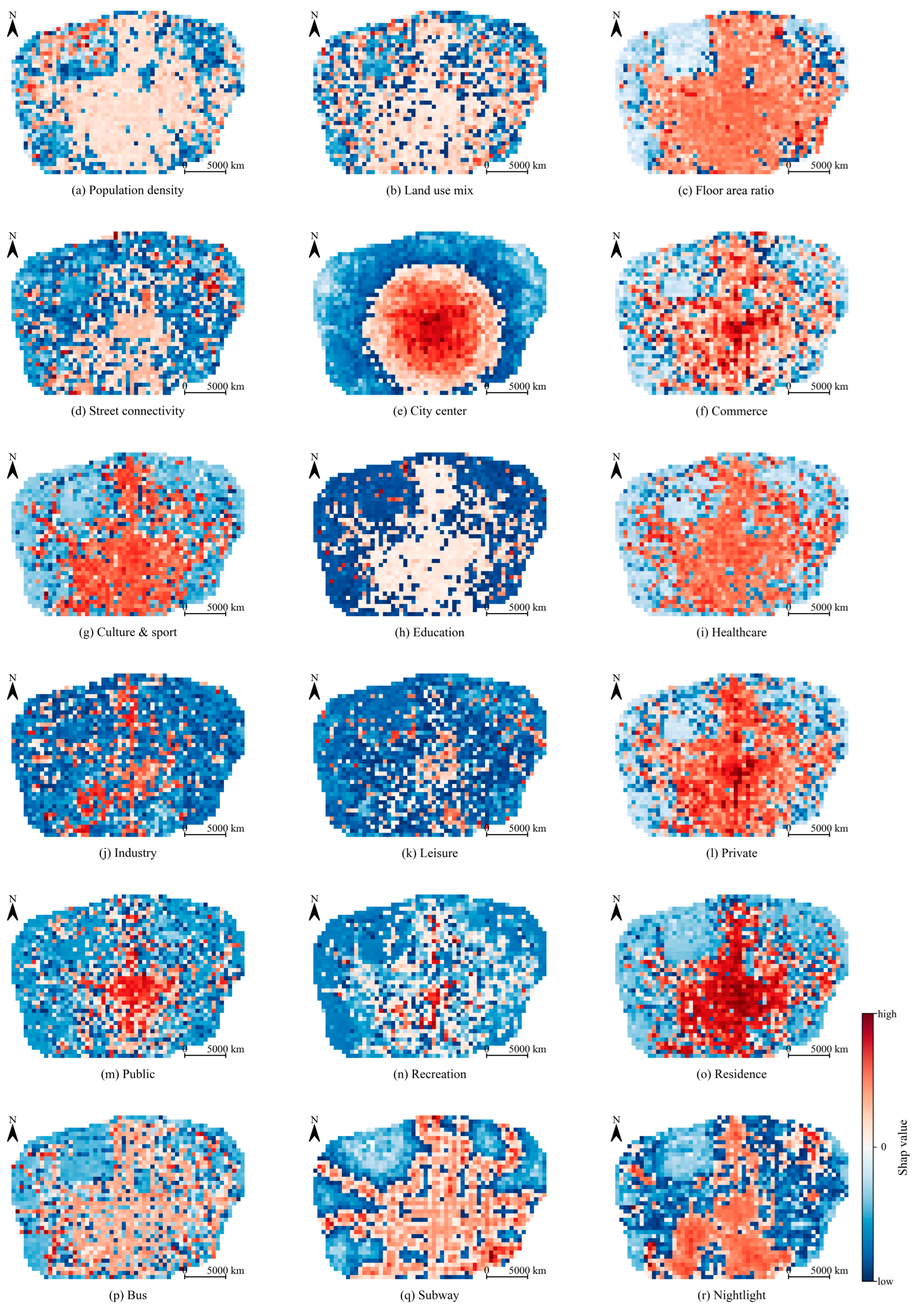
4.5. Spatial Heterogeneity of the Local Effect

In this section, we present the local effects of all the explanatory variables based on random forest. The spatial distribution of the SHAP value for each independent variable is plotted in Figure 6 (HO) and Figure A1 (WO). These show that all factors, including the variables with low global importance, can have an outstanding performance on a local scale. The spatial distributions of the factors’ contributions to predicting HO and WO are significantly similar, which also aligns with Figure 2 and Figure 3. In each explanatory variable, the scatter distribution patterns in the two models are quite similar. Therefore, we only analyze in detail the spatial heterogeneity of the built environment’s local effect on HO to streamline our discussion.
Regarding density, Population density has a greater positive influence on the northwestern corner of the study area and a less positive influence on a large portion of the central part (Figure 6a). Nevertheless, the negative effects are distributed in the peripheral regions. Meanwhile, the positive impact ranges of Land use mix outweigh the negative influence ranges. The contributions to predicting OD flow gathering at the third activity sites have greater positive influences in the south and greater negative influences in the north (Figure 6b). In terms of design, the positive effect area of Floor area ratio is the largest of all the built environment factors and has the best spatial continuity (Figure 6c). The negative effect areas are mainly set outside the positive effect area. In addition, special attention should be paid to the exceptionally low SHAP value for the Daming Palace National Heritage Park. Baqiao is situated at the northeastern corner of the study area, a location where Street connectivity plays a major role (Figure 6d). This area cannot disregard the potential influence of intersections, which facilitate travel.
Significant spatial differences can be observed in the influence of the different variables of destination accessibility on the attraction of the third activity. Figure 6e shows that as the distance to the city center increases, the influence changes from positive to negative, and the SHAP value changes from high to low. Zhonglou and Xiaozhai are commercial centers and are well-equipped with basic amenities. Accordingly, in these areas, Commerce and Private have a strong attraction to the population (Figure 6f,l). The local effects of Culture and sport and Healthcare appear similar, and the area of positive influence is larger in the south (Figure 6g,i). Specifically, the civic and medical facilities are mainly located in the red zone. In terms of Education, the spatial heterogeneity of HO is more significant than that of WO, and the negative SHAP value of WO is smaller compared to that of HO (the blue area in Figure 6h is darker than that in Figure A1h). The small variance in the positive SHAP values can prove that quality educational resources are evenly distributed in the core area of Xi’an. In the central axis and the high-tech zone (the red concentrated areas in Figure 6j), a strong correlation exists between Industry and OD flow gathering at the third activity sites. Leisure and OD flow are negatively correlated (Figure 6k). However, the famous landmarks, such as the Xi’an Circumvallation, Zhonglou, Great Tang all-day mall, Daming Palace National Heritage Park, and the Han Chang’an City Site, attract a large number of tourists. Government agencies and departments are mainly located in the central axis and the old city (the center red areas in Figure 6m), and people visit these places mostly to conduct business. The positive effects of Recreation are mainly observed in certain areas, such as Zhonglou and Xiaozhai, while ultra-low SHAP values are sporadically distributed (Figure 6n). A strong link exists between Residence and population movement in the central region compared to the edge of the study area (Figure 6o).
People rely on public transportation as one of their principal means of travel. The positive effect of Bus is mainly distributed on the trunk roads (Figure 6p). This indicates that bus stops are mainly located on both sides of trunk roads, and the rational layout of bus stops is conducive to attracting population movement. An interesting phenomenon can be found in Figure 6q, where the positive SHAP values are distributed along the subway lines of Xi’an, while the ultra-low SHAP values are embedded around the red region. Meanwhile, red clusters are observed around the southeast corner near the Xi’an Botanical Garden and Yanming Lake leisure park and the northernmost point of the central axis near Daming Palace National Heritage Park and Wangsi subway station. About Others, the substantial residential areas can be found to the north of Three Bridges Street and the north of the median, where the positive effect of Nightlight is evident. Nightlight has also a significant positive influence on the following locations: Zhangbagou Street, which is a hub for industry; Zhonglou, as one of the most famous scenic spots in Xi’an; Yanta District, which also boasts numerous famous attractions, such as Tang Paradise; XIANICEC, which often hosts large events; and Houhai of Chanba, which is a good choice for enjoying a beautiful night view (Figure 6r).

5. Discussion

In our research, random forest was utilized, as a state-of-the-art machine learning model, to uncover fresh perspectives on the nonlinear relationship between the built environment and the attraction of the third activity utilizing fined-grain data that explain the built environment and mobile phone data. We developed an individual random forest model for HO and WO and further interpreted them globally and locally using a SHAP model. In addition, in our study, synergies between each of the two built environment factors were also revealed utilizing PDPs. On this basis, in this work, how the built environment contributes to the attraction of the third activity is revealed. The results of our research provide insights to help policymakers and urban planners optimize communities for participating in the third activity. Based on our findings, policymakers and urban planners can learn more about the effective ranges of the built environment factors, how to enhance the attraction of the third activity in the most cost-effective way, and help other stakeholders, such as real estate developers, understand what type of built environment would attract what type of buyers.
Our findings reflect that although the contributions of all the built environment variables to the attraction of the third activity differ between HO and WO on the global scale, the nonlinear relationships (i.e., partial dependence) and spatial patterns of the SHAP values are highly similar. Accordingly, the global contributions of the built environment to attracting population flow from home and work are different, according to Figure 2 and Figure 3; however, the local effect among them demonstrate a high degree of similarity. In summary, the three most important factors in HO are Private, Floor area ratio, and Healthcare, whereas those in WO are Private, Nightlight, and Residence. Decision makers and urban planners can prioritize the optimization of those built environment factors that are of high importance if they urgently need to improve the degree of people’s attraction to the third activity. Private exhibits the most significant contribution to HO and WO, indicating that amenities providing private services have a greater influence on the attraction of the third activity than other elements. Additionally, people are likely to travel to certain facilities, such as barber shops, laundries, and beauty salons, to meet their needs in daily life. In the context of Xi’an, if a location wants to attract a substantial number of people from their homes, the relevant government departments must rationalize the provision of more facilities of daily life and healthcare services in that place and appropriately increase the floor area ratio. Moreover, a location with a significant number of amenities for day-to-day living and housing and a high Nightlight value is more likely to attract population movement from the workplace.
The SHAP interpreter was used not only to identify the nonlinear effects of explanatory variables on HO and WO but also to visualize the local effect of the built environment variables. In summary, the majority of the features’ global contributions to HO are greater than to WO (Figure 2 and Figure 3). The marginal effects of the built environment factors were unveiled, which can enhance urban planners and government departments’ understanding of how the built environment influences population mobility and effectively assists sustainable urban development and renewal. Specifically, in terms of density, greater attention should be paid by planners to adjust population density to an appropriate level for promoting HO and WO. Once Population density exceeds 28, not only will it fail to enhance the attractiveness of the area for the existing population, but it may also inhibit the inflow of new population members. Overcrowding can cause discomfort for residents. In the northwestern edge of the study area, increasing Population Density could be a good way of attracting people. With regard to diversity, Land use mix is capable of promoting population inflows in general. Planners should rationalize land use mixing because its significant positive and negative effects on population inflow are staggered around the edge of the study area. Land use mix’s significant negative effects on WO have permeated the center region, and this requires further attention. The effective ranges of Floor area ratio and Street connectivity are within 0.8 and 12, respectively. In the Han Chang’an City Site, Daming Palace National Heritage Park, Baqiao, and the southeastern corner of the study area, the high floor area ratio will inhibit population inflow. People visit these places to relax and gain a broad perspective, so the floor area ratio of these places need to be controlled. If three identical triangles are used to delineate the study area, then the number of intersections should be controlled for the upper-left and right triangles, as the high degree of Street connectivity will have an opposite effect. In terms of destination accessibility, all other types of amenities could stimulate the third activity with the exception of City center and Education. For example, although the number of medical facilities shows nuanced effects on HO and WO, its effective range should be between zero and four within a cell, and this observation should be noted by urban designers. Furthermore, the spatial heterogeneity of the different effects varies according to facility type. Transportation authorities must understand that the effects of elements on people’s willingness to travel are nonlinear. The number of bus stops within 18 in a grid is positively related to the attraction of the third activity, while the effect is weaker above this value. The closer people are to a subway station, the more willing they are to travel. All of these findings provide references for TOD planning. The positive effects of Bus and Subway on HO and WO are roughly distributed along the transit lines. Finally, improved economic development could attract the third activity, but this effect has a threshold.
Furthermore, the synergy of the two built environment factors with a higher importance can also have a positive impact on the attraction of the third activity. This synergy may also exhibit a marginal effect, similar to the nonlinear relationship mentioned in our study. Therefore, if the built environment is to be optimized in the most cost-effective way in order to enhance the attraction of the third activity, urban planners must keep the built environment factors within reasonable limits.
In addition, although random forest is one of the most advanced machine learning models, it also suffers from the potential risk of overfitting and the “black-box” problem. Tuning the hyperparameters can avoid overfitting to some extent, while interpretable machine learning models can also help in interpreting complicated models. In our study, neither HO nor WO can be seen to fit the model very well. In terms of the test set, the R2 for HO and WO is 0.532 and 0.538, respectively, implying that our choice of built environment variables explains the attraction of HO to an extent of 53.2% and WO to an extent of 53.8%. This indicates that there are other factors that can have an impact on the attraction of the third activity. More factors could be included for further research in the future.

6. Conclusions

Overall, our research uncovers the global contribution of explanatory variables to HO and WO, disentangles the complex nonlinear relationship between the built environment variables and the attraction of the third activity, and delves into the spatial heterogeneity of these local effects. Additionally, the synergistic effects of each two built environment factors are also further revealed. The findings in this study could help in providing insights and understanding into how the built environment (i.e., the 5Ds) and the state of economic development affect the attraction of the third activity and provide policy implications and spatial planning references for decision makers.
Furthermore, several issues of our research should be further investigated. First, it remains uncertain as to whether the results of this study are generalizable because Xi’an is a monocentric city. In our study, we utilized mobile phone data from only one city due to the limited data. However, the complicated relationship between the attraction of the third activity and the built environment is likely to change over different cities and time periods. Therefore, multi-city and multi-time period studies should be further conducted. Second, although we obtained the best performing model after a number of tuning processes, potential overfitting problems and model uncertainty may remain. If possible, scholars should increase the amount of data and influencing factors for further research in the future. Other models, such as linear or deep learning models, can also be considered for comparative analysis or to improve accuracy. Finally, the intricate relationship we explored between the built environment and attraction to the third activity is more of a correlation than a causal relationship. An inferential model may be needed in the future to explore any causal effects.

Author Contributions

Conceptualization, Lin Luo and Xiping Yang; methodology, Lin Luo, Xiping Yang and Jiayu Liu; writing—original draft preparation, Lin Luo; writing—review and editing, Xiping Yang and Xueye Chen; supervision, Jiayu Liu, Rui An and Jiyuan Li. All authors have read and agreed to the published version of the manuscript.

Funding

This research was funded by the National Natural Science Foundation of China: NO. 42271468, 42101419; the Open Fund of Key Laboratory of Urban Land Resources Monitoring and Simulation, Ministry of Natural Resources: NO. KF2022-07-005.

Data Availability Statement

The data used in this study are available by contacting the first author.

Conflicts of Interest

The authors declare no conflicts of interest.

Appendix A

Figure A1. Spatial distribution of the SHAP main effect values of all explanatory variables (WO).
Ijgi 13 00337 g0a1

References

  1. Wang, Y.; Zhan, Z.; Mi, Y.; Sobhani, A.; Zhou, H. Nonlinear Effects of Factors on Dockless Bike-Sharing Usage Considering Grid-Based Spatiotemporal Heterogeneity. Transp. Res. Part D Transp. Environ. 2022, 104, 103194. [Google Scholar] [CrossRef]
  2. Sun, Y.; Wang, Y.; Wu, H. How Does the Urban Built Environment Affect Dockless Bikesharing-Metro Integration Cycling? Analysis from a Nonlinear Comprehensive Perspective. J. Clean. Prod. 2024, 449, 141770. [Google Scholar] [CrossRef]
  3. Gao, C.; Lai, X.; Li, S.; Cui, Z.; Long, Z. Bibliometric Insights into the Implications of Urban Built Environment on Travel Behavior. ISPRS Int. J. Geo-Inf. 2023, 12, 453. [Google Scholar] [CrossRef]
  4. Yang, X.; Fang, Z.; Yin, L.; Li, J.; Lu, S.; Zhao, Z. Revealing the Relationship of Human Convergence–Divergence Patterns and Land Use: A Case Study on Shenzhen City, China. Cities 2019, 95, 102384. [Google Scholar] [CrossRef]
  5. Tong, Z.; An, R.; Zhang, Z.; Liu, Y.; Luo, M. Exploring Non-Linear and Spatially Non-Stationary Relationships between Commuting Burden and Built Environment Correlates. J. Transp. Geogr. 2022, 104, 103413. [Google Scholar] [CrossRef]
  6. Yang, Y.; Sasaki, K.; Cheng, L.; Liu, X. Gender Differences in Active Travel among Older Adults: Non-Linear Built Environment Insights. Transp. Res. Part D Transp. Environ. 2022, 110, 103405. [Google Scholar] [CrossRef]
  7. Chai, Y. Space–Time Behavior Research in China: Recent Development and Future Prospect: Space–Time Integration in Geography and GIScience. Ann. Assoc. Am. Geogr. 2013, 103, 1093–1099. [Google Scholar] [CrossRef]
  8. Wang, D.; Zhou, M. The Built Environment and Travel Behavior in Urban China: A Literature Review. Transp. Res. Part D Transp. Environ. 2017, 52, 574–585. [Google Scholar] [CrossRef]
  9. Ta, N.; Chai, Y.; Zhang, Y.; Sun, D. Understanding Job-Housing Relationship and Commuting Pattern in Chinese Cities: Past, Present and Future. Transp. Res. Part D Transp. Environ. 2017, 52, 562–573. [Google Scholar] [CrossRef]
  10. Shen, Y.; Ta, N.; Liu, Z. Job-Housing Distance, Neighborhood Environment, and Mental Health in Suburban Shanghai: A Gender Difference Perspective. Cities 2021, 115, 103214. [Google Scholar] [CrossRef]
  11. Mouratidis, K. Built Environment and Leisure Satisfaction: The Role of Commute Time, Social Interaction, and Active Travel. J. Transp. Geogr. 2019, 80, 102491. [Google Scholar] [CrossRef]
  12. Yang, L.; Ao, Y.; Ke, J.; Lu, Y.; Liang, Y. To Walk or Not to Walk? Examining Non-Linear Effects of Streetscape Greenery on Walking Propensity of Older Adults. J. Transp. Geogr. 2021, 94, 103099. [Google Scholar] [CrossRef]
  13. Rout, A.; Nitoslawski, S.; Ladle, A.; Galpern, P. Using Smartphone-GPS Data to Understand Pedestrian-Scale Behavior in Urban Settings: A Review of Themes and Approaches. Comput. Environ. Urban Syst. 2021, 90, 101705. [Google Scholar] [CrossRef]
  14. Wang, D.; Dewancker, B.; Duan, Y.; Zhao, M. Exploring Spatial Features of Population Activities and Functional Facilities in Rail Transit Station Realm Based on Real-Time Positioning Data: A Case of Xi’an Metro Line 2. ISPRS Int. J. Geo-Inf. 2022, 11, 485. [Google Scholar] [CrossRef]
  15. Yang, X.; Li, J.; Fang, Z.; Chen, H.; Li, J.; Zhao, Z. Influence of Residential Built Environment on Human Mobility in Xining: A Mobile Phone Data Perspective. Travel Behav. Soc. 2024, 34, 100665. [Google Scholar] [CrossRef]
  16. Jardim, B.; Neto, M.D.C.; Calçada, P. Urban Dynamic in High Spatiotemporal Resolution: The Case Study of Porto. Sustain. Cities Soc. 2023, 98, 104867. [Google Scholar] [CrossRef]
  17. Liu, X.; Pei, T.; Wang, X.; Liu, T.; Fang, Z.; Jiang, L.; Jiang, J.; Yan, X.; Wu, M.; Peng, Y.; et al. Travel Flow Patterns of Diverse Population Groups and Influencing Built Environment Factors: A Case Study of Beijing. Cities 2024, 151, 105096. [Google Scholar] [CrossRef]
  18. Kraft, S.; Halás, M.; Klapka, P.; Blažek, V. Functional Regions as a Platform to Define Integrated Transport System Zones: The Use of Population Flows Data. Appl. Geogr. 2022, 144, 102732. [Google Scholar] [CrossRef]
  19. Rui, J. Exploring the Association between the Settlement Environment and Residents’ Positive Sentiments in Urban Villages and Formal Settlements in Shenzhen. Sustain. Cities Soc. 2023, 98, 104851. [Google Scholar] [CrossRef]
  20. Zhang, X.; Zhou, Z.; Xu, Y.; Zhao, X. Analyzing Spatial Heterogeneity of Ridesourcing Usage Determinants Using Explainable Machine Learning. J. Transp. Geogr. 2024, 114, 103782. [Google Scholar] [CrossRef]
  21. Liu, J.; Meng, B.; Yang, M.; Peng, X.; Zhan, D.; Zhi, G. Quantifying Spatial Disparities and Influencing Factors of Home, Work, and Activity Space Separation in Beijing. Habitat Int. 2022, 126, 102621. [Google Scholar] [CrossRef]
  22. Gong, L.; Jin, M.; Liu, Q.; Gong, Y.; Liu, Y. Identifying Urban Residents’ Activity Space at Multiple Geographic Scales Using Mobile Phone Data. ISPRS Int. J. Geo-Inf. 2020, 9, 241. [Google Scholar] [CrossRef]
  23. Zheng, Z.; Zhou, S.; Deng, X. Exploring Both Home-Based and Work-Based Jobs-Housing Balance by Distance Decay Effect. J. Transp. Geogr. 2021, 93, 103043. [Google Scholar] [CrossRef]
  24. Li, Y.; Yao, E.; Liu, S.; Yang, Y. Spatiotemporal Influence of Built Environment on Intercity Commuting Trips Considering Nonlinear Effects. J. Transp. Geogr. 2024, 114, 103744. [Google Scholar] [CrossRef]
  25. Zhang, Y.; Song, Y.; Zhang, W.; Wang, X. Working and Residential Segregation of Migrants in Longgang City, China: A Mobile Phone Data-Based Analysis. Cities 2024, 144, 104625. [Google Scholar] [CrossRef]
  26. Jin, S.T.; Wang, L.; Sui, D. How the Built Environment Affects E-Scooter Sharing Link Flows: A Machine Learning Approach. J. Transp. Geogr. 2023, 112, 103687. [Google Scholar] [CrossRef]
  27. Yin, G.; Huang, Z.; Fu, C.; Ren, S.; Bao, Y.; Ma, X. Examining Active Travel Behavior through Explainable Machine Learning: Insights from Beijing, China. Transp. Res. Part D Transp. Environ. 2024, 127, 104038. [Google Scholar] [CrossRef]
  28. Yang, H.; Zhang, Q.; Helbich, M.; Lu, Y.; He, D.; Ettema, D.; Chen, L. Examining Non-Linear Associations between Built Environments around Workplace and Adults’ Walking Behaviour in Shanghai, China. Transp. Res. Part A Policy Pract. 2022, 155, 234–246. [Google Scholar] [CrossRef]
  29. Gao, K.; Yang, Y.; Li, A.; Qu, X. Spatial Heterogeneity in Distance Decay of Using Bike Sharing: An Empirical Large-Scale Analysis in Shanghai. Transp. Res. Part D Transp. Environ. 2021, 94, 102814. [Google Scholar] [CrossRef]
  30. Lyu, T.; Wang, Y.; Ji, S.; Feng, T.; Wu, Z. A Multiscale Spatial Analysis of Taxi Ridership. J. Transp. Geogr. 2023, 113, 103718. [Google Scholar] [CrossRef]
  31. Venkadavarahan, M.; Joji, M.S.; Marisamynathan, S. Development of Spatial Econometric Models for Estimating the Bicycle Sharing Trip Activity. Sustain. Cities Soc. 2023, 98, 104861. [Google Scholar] [CrossRef]
  32. Credit, K.; O’Driscoll, C. Assessing Modal Tradeoffs and Associated Built Environment Characteristics Using a Cost-Distance Framework. J. Transp. Geogr. 2024, 117, 103870. [Google Scholar] [CrossRef]
  33. Zhao, B.; Deng, M.; Shi, Y. Inferring Nonwork Travel Semantics and Revealing the Nonlinear Relationships with the Community Built Environment. Sustain. Cities Soc. 2023, 99, 104889. [Google Scholar] [CrossRef]
  34. Tu, M.; Li, W.; Orfila, O.; Li, Y.; Gruyer, D. Exploring Nonlinear Effects of the Built Environment on Ridesplitting: Evidence from Chengdu. Transp. Res. Part D Transp. Environ. 2021, 93, 102776. [Google Scholar] [CrossRef]
  35. Li, Z. Leveraging Explainable Artificial Intelligence and Big Trip Data to Understand Factors Influencing Willingness to Ridesharing. Travel Behav. Soc. 2023, 31, 284–294. [Google Scholar] [CrossRef]
  36. Gao, K.; Yang, Y.; Gil, J.; Qu, X. Data-Driven Interpretation on Interactive and Nonlinear Effects of the Correlated Built Environment on Shared Mobility. J. Transp. Geogr. 2023, 110, 103604. [Google Scholar] [CrossRef]
  37. Liu, X.; Chen, X.; Tian, M.; De Vos, J. Effects of Buffer Size on Associations between the Built Environment and Metro Ridership: A Machine Learning-Based Sensitive Analysis. J. Transp. Geogr. 2023, 113, 103730. [Google Scholar] [CrossRef]
  38. Osorio-Arjona, J.; García-Palomares, J.C. Social Media and Urban Mobility: Using Twitter to Calculate Home-Work Travel Matrices. Cities 2019, 89, 268–280. [Google Scholar] [CrossRef]
  39. Liu, Y.; Li, Y.; Yang, W.; Hu, J. Exploring Nonlinear Effects of Built Environment on Jogging Behavior Using Random Forest. Appl. Geogr. 2023, 156, 102990. [Google Scholar] [CrossRef]
  40. Lv, H.; Li, H.; Chen, Y.; Feng, T. An Origin-Destination Level Analysis on the Competitiveness of Bike-Sharing to Underground Using Explainable Machine Learning. J. Transp. Geogr. 2023, 113, 103716. [Google Scholar] [CrossRef]
  41. Zheng, S.; Zheng, J. Assessing the Completeness and Positional Accuracy of OpenStreetMap in China. In Thematic Cartography for the Society; Bandrova, T., Konecny, M., Zlatanova, S., Eds.; Springer International Publishing: Cham, Germany, 2014; pp. 171–189. ISBN 978-3-319-08180-9. [Google Scholar]
  42. Castro, R.; Tierra, A.; Luna, M. Assessing the Horizontal Positional Accuracy in OpenStreetMap: A Big Data Approach. In New Knowledge in Information Systems and Technologies; Rocha, Á., Adeli, H., Reis, L.P., Costanzo, S., Eds.; Springer International Publishing: Cham, Switzerland, 2019; pp. 513–523. [Google Scholar]
  43. Wu, F.; Li, W.; Qiu, W. Examining Non-Linear Relationship between Streetscape Features and Propensity of Walking to School in Hong Kong Using Machine Learning Techniques. J. Transp. Geogr. 2023, 113, 103698. [Google Scholar] [CrossRef]
  44. Ewing, R.; Cervero, R. Travel and the Built Environment: A Meta-Analysis. J. Am. Plan. Assoc. 2010, 76, 265–294. [Google Scholar] [CrossRef]
  45. Yue, Y.; Zhuang, Y.; Yeh, A.G.O.; Xie, J.-Y.; Ma, C.-L.; Li, Q.-Q. Measurements of POI-Based Mixed Use and Their Relationships with Neighbourhood Vibrancy. Int. J. Geogr. Inf. Sci. 2017, 31, 658–675. [Google Scholar] [CrossRef]
  46. Breiman, L. Random Forests. Mach. Learn. 2001, 45, 5–32. [Google Scholar] [CrossRef]
  47. Lundberg, S.M.; Lee, S.-I. A Unified Approach to Interpreting Model Predictions. arXiv 2017, arXiv:1705.07874. [Google Scholar]
  48. Shapley, L.S. A Value for N-Person Games; RAND Corporation: Santa Monica, CA, USA, 1952. [Google Scholar]
  49. Molnar, C. Interpretable Machine Learning; Leanpub: Victoria, BC, Canada, 2020. [Google Scholar]
  50. Hastie, T.; Tibshirani, R.; Friedman, J. The Elements of Statistical Learning; Springer Series in Statistics; Springer: New York, NY, USA, 2009; ISBN 978-0-387-84857-0. [Google Scholar]
Figure 1. Study area: (a) details of the selected zone; (b) overview of Xi’an.
Ijgi 13 00337 g001
Figure 2. Relative importance of explanatory variables for the global and local explanations (HO).
Ijgi 13 00337 g002
Figure 3. Relative importance of explanatory variables for the global and local explanations (WO).
Ijgi 13 00337 g003
Figure 4. Nonlinear relationship between the built environment and OD flow (HO and WO): (ar) nonlinear effects of each built environment factor.
Ijgi 13 00337 g004
Figure 5. Synergy of each of the two built environment factors on the attraction of the third activity.
Ijgi 13 00337 g005
Figure 6. Spatial distribution of the SHAP main effect values of all explanatory variables (HO).
Ijgi 13 00337 g006
Table 1. Definition and descriptive statistics of all variables.
VariableDescriptionMeanStd.MinMax
OD flow
A i h Natural logarithm of home–other flow4.286 2.412 08.635
A i w Natural logarithm of work–other flow4.023 2.436 0 8.786
Density
Population densityAverage number of people per cell31.888 23.761 0 524.882
Diversity
Land use mixLand use entropy index of multiple types of POIs: E n t r o p y = i = 1 s p i ln p i ln s , where p i is the ratio of the i th type of POI in each cell, and s is the number of types of POIs (s = 10)0.539 0.206 0 0.876
Design
Floor area ratioRatio of the total floor area of all buildings to the area of each cell: F l o o r   a r e a   r a t i o = i = 1 j A i F i A , where A i and F i are the area and number of floors of the building footprint i , respectively, and A indicates the total area of the cell 0.811 0.789 0 3.799
Street connectivityNumber of road intersections in each cell7.593 9.328 0 139
Destination accessibility
City centerEuclidean distance from the geometric center of each cell to the city center (km)8.649 3.393 0.180 15.639
CommerceNumber of commercial POIs (e.g., supermarkets, shopping malls) in each cell83.667 169.836 0 2387
Culture and sportNumber of cultural and sport POIs in each cell7.430 11.998 0 132
EducationNumber of POIs for schools and educational facilities in each cell1.395 2.526 0 37
HealthcareNumber of POIs for hospitals, clinics, and pharmacies in each cell5.874 8.335 0 83
IndustryNumber of POIs for enterprises in each cell12.277 22.245 0 237
LeisureNumber of POIs for parks and landscapes in each cell0.643 2.283 0 42
PrivateNumber of POIs providing private services to people in their daily life in each cell (e.g., barber shops, beauty salons, laundries, and mobile business halls)31.854 49.715 0 676
PublicNumber of POIs for public facilities and government agencies5.459 8.488 0 109
RecreationNumber of recreational POIs (e.g., internet cafés and chess rooms) in each cell1.868 5.762 0 118
ResidenceNumber of residential POIs in each cell4.559 6.088 0 41
Distance to transit
Bus Number of bus stops in each cell7.420 9.069 0 52
SubwayEuclidean distance from the geometric center of each cell to the nearest metro station (km)1.223 1.065 0.006 6.245
Others
NightlightAverage value of nightlight for each cell56,761.347 61,156.766 1710.800 670,362
Note: the total sample size is 1920 OD pairs.
Table 2. Model performance metrics.
ModelTraining SetTest Set
R2MSEMAER2MSEMAE
HO0.6551.9721.1110.5322.8951.353
WO0.6811.8481.0930.5382.9681.397
Disclaimer/Publisher’s Note: The statements, opinions and data contained in all publications are solely those of the individual author(s) and contributor(s) and not of MDPI and/or the editor(s). MDPI and/or the editor(s) disclaim responsibility for any injury to people or property resulting from any ideas, methods, instructions or products referred to in the content.

