Interpretable Machine Learning Insights into the Factors Influencing Residents’ Travel Distance Distribution

Abstract

Understanding intra-urban travel patterns through quantitative analysis is crucial for effective urban planning and transportation management. In previous studies, a range of distribution functions were modeled to lay the groundwork for human mobility research. However, few studies have explored the nonlinear relationships between travel distance patterns and environmental factors. Using travel distance data from ride-hailing services, this research divides a study area into 1 × 1 km grid cells, modeling the best travel distance distribution and calculating the coefficients of each grid. A machine learning framework (Extreme Gradient Boosting combined with Shapley Additive Explanations) is introduced to interpret the factors influencing these distributions. Our results emphasize that the travel distance of human movement tends to follow a log-normal distribution and exhibits spatial heterogeneity. Key factors affecting travel distance distributions include the distance to the city center, bus station density, land use entropy, and the density of companies. Most environmental variables exhibit nonlinear and threshold effects on the log-normal distribution coefficients. These findings significantly advance our understanding of ride-hailing travel patterns and offer valuable insights into the spatial dynamics of human mobility.

1. Introduction

Comprehending, modeling, and forecasting human movement within urban environments is an essential task for various domains and applications, including human behavior [1], transportation and activity analysis [2], and urban planning [3]. Modeling the distributions of fundamental indicators is essential for investigating latent mobility patterns and serves as a critical foundation for advancing research in human mobility [4,5,6]. The recent accessibility of extensive datasets on human movement and behavior has facilitated the creation and validation of human mobility models [7]. Numerous empirical studies have shown that mobility metrics can be effectively represented using significant distributions.

Studies have used different means of modeling individual travel metrics. A statistical examination of banknote trajectories indicated that the displacement distribution closely follows a power-law approximation [8]. González and colleagues performed a statistical examination of human movement patterns, analyzing six months of call detail records (CDR) from almost 100,000 anonymous mobile phone users. They discovered that the distances traveled by these individuals typically follow a power-law distribution, which is truncated by an exponential function [1]. Jiang analyzed the GPS traces of 50 taxis across four Swedish cities over a six-month period, discovering that the travel distances of cab riders follow a bimodal power-law distribution [2]. Liang et al. investigated a larger-scale dataset of taxi trip distances and found that the travel distances had an exponential distribution [9]. Individual traveler characteristics, extracted from private vehicle data, indicated that trip distances approximate an exponential distribution [10,11]. Using data from online social networks [12,13,14] and GPS trajectories [9,15], it was found that the displacement distribution can be well represented using an exponential curve, particularly for short distances. Additionally, analyses of GPS data from taxis [16,17] indicated that displacements might also conform to log-normal distributions. Differences in the conclusions of these studies may arise from the use of different datasets and inconsistencies in the datasets covering the groups. The modeling and empirical results for current travel distance distributions are mainly summarized as power-law, power law with exponential cutoff, exponential, log-normal, and other functions.

Existing datasets in the literature include, but are not limited to, call detail records (CDRs), location-based social network data (LBSN), GPS trajectories of vehicles, and card-swipe records from public transportation systems such as buses or subways. However, there is currently no consensus on which distribution best describes these empirical datasets. Ride-hailing, as an emerging mode of transportation, shares similarities with traditional taxis in external form but remains underexplored as an empirical dataset in mobility studies due to its relatively recent adoption [18,19]. Online ride-hailing datasets are distinguished by their high quality, fine-grained resolution, and extensive scale, effectively recording precise spatiotemporal trajectories alongside actual trip origins and destinations. Consequently, these services present a comprehensive and reliable data source for distribution modeling, creating fresh opportunities and challenges for enhancing insights into human travel patterns and urban mobility dynamics.

The impact of the built environment on human mobility cannot be overlooked, as it significantly influences how individuals navigate within and engage with urban environments. Since the early days of travel behavior research, the relationship between travel patterns and the built environment has been a central topic of investigation. Components including land use, infrastructure, and urban density are known to influence how people make travel decisions, including their choice of transport mode, route, and travel frequency [20,21,22]. These studies typically use survey data to capture the interplay between human behavior and the built environment, providing valuable insights into how localized urban features can either facilitate or constrain mobility choices. Research on collective human mobility patterns has frequently concentrated on exploring the overarching connection of the built environment and spatiotemporal dynamics, as well as urban vitality. This includes investigating how factors such as land use diversity, functional zoning, and the distribution of public spaces impact human movement and activity levels across larger urban areas [23,24,25]. These studies explore how different urban designs and layouts can foster increased human interaction and dynamic mobility, contributing to a city’s vibrancy and economic productivity. However, most previous studies have concentrated on general mobility patterns rather than deeply analyzing travel metric distributions in different urban settings.

Traditional regression techniques like Ordinary Least Squares (OLS) and Random Forest (RF) are commonly used to explore influential urban factors, yet they often face challenges of overfitting or underfitting with urban datasets. Additionally, Prior research typically employed methods such as Variable Relative Importance (RI) [26] and Partial Dependence Plots (PDPs) [27] to illustrate broad relationships among variables; however, these approaches do not adequately meet the demand for localized explanations in diverse spatial contexts. This limitation contributes to the "black box” character of conventional machine learning models, obscuring a detailed understanding of factor impacts on specific local urban settings.

Previous work in this area has several significant limitations that need to be addressed: (1) Prior research ignored the spatial heterogeneity of distance distributions using ride-hailing and was therefore inefficient in depicting divergences in distance distributions across different urban contexts. (2) Relatively few studies have utilized large-scale spatiotemporal datasets to specifically examine how the built environment influences human travel distances across various urban contextsc [28] and to empirically uncover the mechanisms behind the spatial variations in distance distributions. (3) It remains unclear how these factors differ in their nonlinear relationships with travel distances. (4) Finally, Previous studies commonly used methods like RI and PDPs to explore broad variable relationships, yet these techniques lack the capability to provide detailed explanations specific to individual spatial units.

To bridge these gaps, this study seeks to analyze the nonlinear association between the built environment and distance distribution coefficients using extensive ride-hailing data and machine learning models. First, the data are preprocessed, and the relevant city is divided into a 1 × 1 km grid. Second, the probability distribution function (PDF) of travel distances in different urban contexts is empirically estimated. Third, the influence of various variables on the parameters of probability distribution related to ride-hailing usage is examined using Extreme Gradient Boosting (XGBoost), leveraging multivariate data from emerging technological tools. Fourth, Shapley Additive Explanations (SHAP) analysis is conducted to uncover the differences in how factors influence the fitting parameters.

As a result, the main goals of this study are outlined as follows: (1) To quantify the movement distances of residents and group them based on grids, with the probability density functions (PDFs) in different urban contexts based on the ride-hailing trips; (2) to reveal the relative significance of built environment features to the distribution of travel distances; (3) to elucidate the nonlinear and threshold effects of explanatory factors on the distribution of travel distances; and (4) to provide insights into urban mobility for urban planners and policymakers.

The following sections of this paper are organized as follows: Section 2 outlines the method for assessing appropriate formulas, computing built environment indicators, and specifying models for XGBoost and SHAP. Section 3 details the findings, Section 4 explores the discussion, and Section 5 offers concluding remarks.

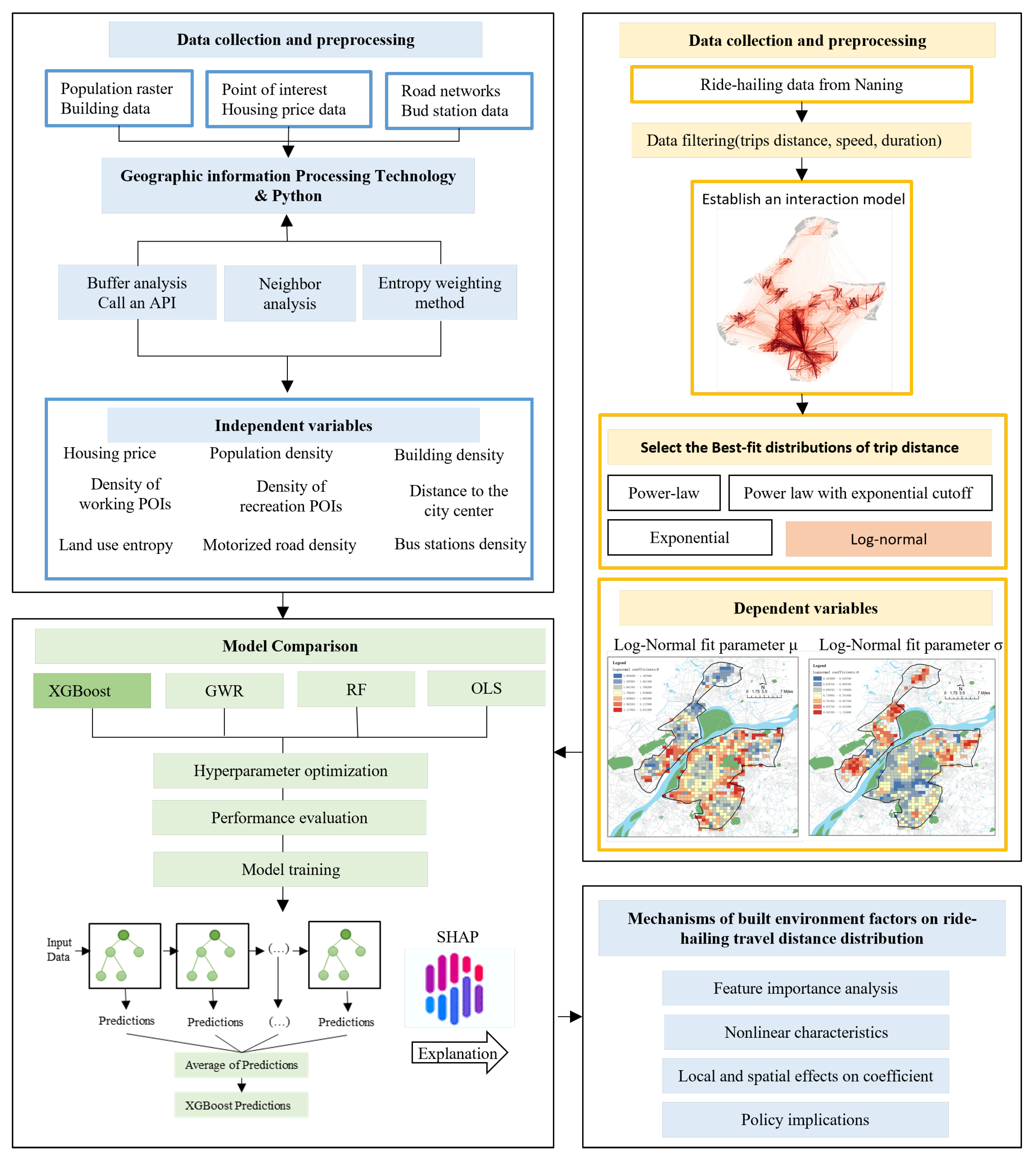
2. Materials and Methods

2.1. Study Area and Data Sources

We established a conceptual framework to assess the non-linear relationships between intra urban distance distribution and factors such as socio-demographic characteristics, facility accessibility, construction density, and traffic connectivity. Figure 1 illustrates the framework, which involves both data preparation and analysis. The first step, data preparation, includes gathering ride-hailing data, population statistics, POI details, and other relevant datasets. Prior to analysis, the data was aggregated into 1 × 1 km grids. The probability density function (PDF) of travel distances across various urban environments was then empirically estimated. Subsequently, the significance of explanatory variables, along with the identification of non-linear effects and thresholds, was analyzed using the most accurate machine learning models and SHAP values. The subsequent subsection offers an in-depth description of the data and methodology.

2.1.1. Study Area

Nanjing serves as the capital of Jiangsu Province, covering a land area of 6582.31 square kilometers and boasting a resident population of 9,491,100. With an urbanization rate of 86.9% and one of the highest levels of socio-economic development in China, it has diverse urban functions and exhibits strong spatial heterogeneity.

We selected the city center districts as the study area (Figure 2). The studied area encompasses diverse urban contexts, comprising both municipal areas and natural environments such as forests and water bodies. The city center is significantly influenced by the surrounding natural landscape and feature distinct spatial functional layouts. Although the city center occupies only 12% of the total area, it is home to 80% of the population. It stretches 54.53 km from south to north and 40.86 km from east to west. The city center districts are well equipped with residential facilities and employment opportunities, accommodating the majority of residents’ daily life and work activities, making them ideal locations for studying human mobility patterns.

2.1.2. Data Sources

The ride-sourcing order data encompassed all trips in Nanjing from 6 March to 12 March 2023. Each order consists of a sequence of data encompassing nine fields: an anonymized order ID, the longitude and latitude of both the pick-up and drop-off points, the start and stop times of each trip, the driving distance, and the driving time (

Table 1. Data selection after processing.

Field	Type	Example
Order ID	Int	35,295,630,329,820
Pick-up longitude	Float	119.03238
Pick-up latitude	Float	31.631422
Drop-off longitude	Float	119.177723
Drop-off latitude	Float	31.575701
Pick-up time stamp	Int	1,676,824,955
Drop-off time stamp	Int	1,676,826,093
Miles driven	Float	18.14
Driving time	Float	19

). The dataset comprises over 2 million ride-sourcing trips, covering a comprehensive geographic spread across the metropolitan area and representing a wide demographic spectrum of users. This substantial data volume ensures a robust basis for analyzing urban mobility patterns within the context of ride-sourcing services. However, the demographic profile of ride-sourcing users, typically younger and more affluent, may not accurately reflect the broader population [29], which could skew the insights into overall urban mobility patterns. Thus, the study could potentially overestimate or underestimate the impact of specific built environment factors.

To assess built environment indicators across all analysis zone, we utilized the Gaode Web Map Service Platform (http://lbs.amap.com/) as our primary data source. Through this platform, we collected information on 14 distinct categories of Points of Interest (POIs) (Appendix A

Table A1. POI categories.

Land Use Categories	Code	POI Category
Working POI	1	Governmental organizations
	2	Social communities
	3	Schools and educational institutions
	4	Company and business
Recreation POI	5	Restaurants
	6	Coffee/tea shops
	7	Sports stadiums
	8	Tourism spots
	9	Cultural venues
	10	Recreation stores and centers
	11	Supermarkets
	12	Shopping malls
	13	Parks/squares
	14	Hotels

) and building-related attributes, such as building heights. After conducting rigorous data cleaning, including the removal of duplicates and filtering to focus exclusively on the study area, our dataset comprised 288,512 unique buildings and 572,951 individual POIs. This extensive dataset offers a thorough depiction of the spatial and structural attributes of the urban landscape, crucial for precise analysis.

We utilized a second-hand housing price dataset obtained from Beike (https://m.ke.com/), one of China’s largest companies offering map-based searches for comprehensive housing property coverage. The dataset employed in this research contains information collected in 2023 on thousands of residential properties in Nanjing.

Demographic data were obtained from the World of Pop database (https://www.worldpop.org/), according to The Statistical Yearbook of Chengdu Cityin 2016 and 2017 to adjust the calibration. Administrative division data were sourced from the National Catalogue Service for Geographic Information website (https://www.webmap.cn/), while road network data were obtained from OpenStreetMap (https://www.openstreetmap.org/).

2.2. Variables

2.2.1. Dependent Variables

Data cleaning proved indispensable, as several trip records were deemed unsuitable for inclusion in this study. As a result, it was crucial to remove datasets that exhibited abnormal operations, including duplicates, missing data and overflow. Additionally, considering citizens’ travel patterns and urban area characteristics, we established criteria: (1) distances spanning from 1 to 100 km; (2) travel durations under 1 min or exceeding 2 h; (3) a Average speeds slower than 5 km/h or faster than 80 km/h, and (4) the positions of the origin and destination outside the study area limits [30]. Excluding records according to the specified criteria resulted in 1,935,704 entries deemed suitable for this study.

Drawing from the spatial characteristics of the study area and consulting previous research findings [31], we established 1 × 1 km grids. Consequently, the study area was divided into 630 grids. Interaction networks were established using the centroids of the grids. The next step was to allocate the distance data into statistical 1 × 1 km grids using cell coverage area centroids. In this context, the travel distance pertains to the actual length of the route traversed by the origin–destination trip within road networks. Data preprocessing was finalized with the elimination of nets containing fewer than 200 interactions to optimize the representational efficiency of the curve.

The optimal model parameters were selected as the dependent variable. The aim of selecting a fitting function is to determine the most suitable distribution based on empirical trip data.

Table 2. Functions and parameters of some common probability distributions.

Distribution	Distribution Function and Normalization Constant * $\mathit{p}\left(\mathit{x}\right)=\mathit{Cf}\left(\mathit{x}\right)$
	$\mathit{f}\left(\mathit{x}\right)$	$\mathit{C}$
Power law	$x^{-\alpha }$	$(\alpha -1)x_{min}^{\alpha -1}$
Power law with exponential cutoff	$x^{-\alpha }{e}^{-\lambda x}$	${\displaystyle \frac{{\lambda }^{1-\alpha }}{\mathrm{\Gamma }(1-\alpha ,\lambda x_{min})}}$ **
Exponential	$e^{-\lambda x}$	$\lambda e^{-\lambda x_{min}}$
Log-normal	${\displaystyle \frac{1}{x}}{e}^{-{\displaystyle \frac{{(lnx-\mu )}^2}{2{\sigma }^2}}}$	$\sqrt{{\displaystyle \frac{2}{\pi {\sigma }^2}}}{\left[erfc(-{\displaystyle \frac{ln{x}_{min}-\mu }{\sqrt{2}\sigma }})\right]}^{-1}$ ***

* for each distribution, the basic function form $f\left(x\right)$ and appropriate normalization constant C are given for the continuous case such that ${\int }_{x_{min}}^{\infty }Cf\left(x\right)dx=1$. ** $\mathrm{\Gamma }(·)$ represents the upper incomplete gamma function (upper incomplete gamma function). *** $erfc(·)$ represents the complementary Gaussian error function (complementary Gaussian error function).

presents a range of common probability distribution functions (PDFs) found in prior research, encompassing exponential, power-law, lognormal, and truncated power-law distributions. The parameters were fitted through maximum likelihood estimation (MLE), with comprehensive guidance [32]. Additionally, the table provides formulas for expectation and variance, which are pivotal for discerning distribution characteristics. The Akaike weights $w_i$ for the four models were calculated based on the Akaike Information Criterion (AIC). The model with the highest Akaike weight $w_i$ was considered to have the best-fitting distribution.

In addition, the Akaike information criterion (AIC) can provide another decision-making method. The AIC score is a function of its maximized log-likelihood ($L_i$) and the number of estimated parameters ($K_i$) for each candidate model i, and it is calculated as follows:

$$AI{C}_i=-2·ln{L}_i+2·K_i$$

(1)

The relative likelihood of the model is represented by the weight $w_i$, which is defined as follows:

$$AI{C}_{min}=min\left\{AI{C}_i\right\}$$

(2)

$${\mathrm{\Delta }}_i=AI{C}_i-AI{C}_{min}$$

(3)

$$w_i={\displaystyle \frac{e^{-{\mathrm{\Delta }}_i/2}}{{\sum }_{j=1}^N{e}^{-{\mathrm{\Delta }}_j/2}}}$$

(4)

The largest model i is most likely to be selected. The optimal model has the smallest $AI{C}_i$ (i.e., $AI{C}_{min}$) and the largest contribution to the denominator. Therefore, its weight $w_i$ is close to 1.

2.2.2. Independent Variables

Table 3. Variable descriptions and descriptive statistics.

Variable	Abbreviation	Description	Mean	Standard Deviation	Source
Socio-demographic characteristics
Housing price (ten thousand CNY/km2)	HP	The average value of second-hand housing prices within each analysis zone.	2.2713	1.7595	[33,34]
Population density (person/km2)	PD	The population divided by the total area within each analysis zone.	7721.7519	9372.4370	[33,34]
Facility Convenience
Distance to the city center (m)	DCC	The distance to the nearest city center.	9444.6175	4415.8310	[35]
Density of working POIs (numbers/km2)	DWP	Number of working facilities divided by the total area within each analysis zone.	1591.4286	1739.9334	[34,36]
Density of recreation POIs (numbers/km2)	DRP	The number of recreation facilities divided by total area within each analysis zone.	817.4651	665.3297	[34,36]
Construction intensity
Building density	BD	The ratio of the total building base area to the total land area within each analysis zone.	0.1425	0.0876	[34]
Land use entropy	LUE	The mixed status of POIs within the analysis zone.	0.7673	0.1369	[33,34,36]
Traffic accessibility
Motorized road density (km)	MD	The length of primary and secondary roads available for ride-hailing in each analysis zone.	7.2065	3.3221	[37]
Bus station density (numbers/km2)	BSD	The number of bus stations in each analysis zone.	4.4079	3.0891	[38]

outlines the independent variables, which are divided into four categories: socio-demographic characteristic, facility convenience, construction intensity and traffic accessibility. This provides a holistic framework for analyzing urban dynamics. The definitions and calculation methods for the built environment factors are detailed in Table 3, with measurements obtained separately within each network.

Distance to the city center: City centers were identified via population raster, and the actual distance from each analysis zone particle to the nearest city center was calculated by the Gaode API. We assumed that the routes recommended by Gaode map closely reflect the routes most individuals would realistically adopt. Python scripts were used to access the Gaode map API developer portal to extract driving routes for all trips. The API provided outputs such as the trajectory of the recommended route and the total distance of each trip, allowing us to calculate the plausible driving distances for each journey.

Land use entropy: The larger the entropy value, the more evenly distributed the functions of various facilities in the street, and the smaller the entropy value, the lower the degree of mixed functions.

$$MixUse{d}_k=-{\displaystyle \frac{{\displaystyle \sum _{i=1}^M{P}_{k,i}ln{P}_{ki}}}{lnM}}$$

(5)

$p_{ki}$ is the proportion of the number of Class i POIs in cell k to the number of POIs in the current space cell, and M is the type of POI in the current space cell.

2.3. Data Processing and Modeling

To establish robust regression models, we initiated our analysis by evaluating multicollinearity among the independent variables. Following the guidelines outlined by W. Yang et al. [28] and Yi et al. [39], we confirmed that all variables had a variance inflation factor (VIF) below 10, allowing us to retain all variables in the analysis without concern for multicollinearity. In contrast, for nonlinear and nonparametric approaches such as XGBoost, the issue of multicollinearity is less critical. This flexibility permitteds us to retain all independent variables in our analysis, as highlighted by Luo et al. [40]. Following this, we divided the dataset into training and testing sets, using a 7:3 ratio to improve model validation. To counter potential overfitting and enhance model performance, we implemented 10-fold cross-validation [41]. This method divides the dataset into ten distinct subsets, utilizing one subset for validation while the others contribute to the training process, iteratively rotating through all subsets. For parameter optimization within the XGBoost model, we employed Grid Search, allowing us to systematically explore a range of parameter configurations. In addition to using XGBoost, we experimented with OLS, GWR and RF models to identify the method that provided the greatest predictive accuracy for our specific application. This comparative analysis ensured that the selected model aligned with the characteristics of our dataset and research objectives, enhancing the reliability of our findings. The entire regression analysis was conducted using Python, ensuring a comprehensive and replicable methodology.

2.4. XGBoost Model and SHAP

In machine learning, the gradient boosting decision tree algorithm has the capability to predict outcomes for new input data by learning from training data and detecting trends. This approach offers numerous advantages, making it a popular choice among researchers in the age of big data for elucidating data patterns and achieving precise predictions. XGBoost diverges from traditional gradient boosting methods that utilize gradient descent in function space by employing a technique similar to the Newton-Raphson method. This method involves using a second-order Taylor expansion of the loss function, which allows for more accurate updates and quicker convergence.This nuanced optimization strategy enhances both the efficiency and accuracy of the model. This approach has proven effective in clarifying the influence of various urban elements on phenomena like urban vitality [42] and transportation [43].

SHAP (SHapley Additive exPlanations) is a method grounded in game theory for interpreting machine learning models. It calculates an importance value for each feature in a model, termed the SHAP value, by equitably distributing the model’s prediction output among all input features. These values stem from the Shapley value concept in cooperative game theory, which guarantees that the contributions of all potential feature combinations are considered. SHAP accounts for feature interactions by assessing how the inclusion or exclusion of each feature in various subsets influences the model’s prediction accuracy. This method offers both local explanations for individual predictions and global insights that apply to the entire dataset. Due to its ability to ensure consistency and accuracy, SHAP has become a widely used tool for elucidating complex models such as neural networks and gradient boosting machines.

The Shapley value for a specific feature i is defined as the weighted sum of its marginal contributions across all possible combinations of features. It is formulated as follows:

$${\varphi }_i=\sum _{S\subseteq N}{\displaystyle \frac{\left|S\right|!(n-|S|-1)!}{n!}}[v(S\cup \left\{i\right\})-v\left(S\right)]$$

(6)

Here, $\left|S\right|$ signifies the number of features in a subset S. n is the total count of features, $v\left(s\right)$ is the model prediction with the current set of features, and $v(S\cup i)$ is the prediction when feature i is added to the subset S. By applying this method, we delve into the specific contributions of each independent variable to the prediction, providing nuanced insights that are instrumental for urban planning and policy making.

3. Results

3.1. Spatial Distribution of Coefficients

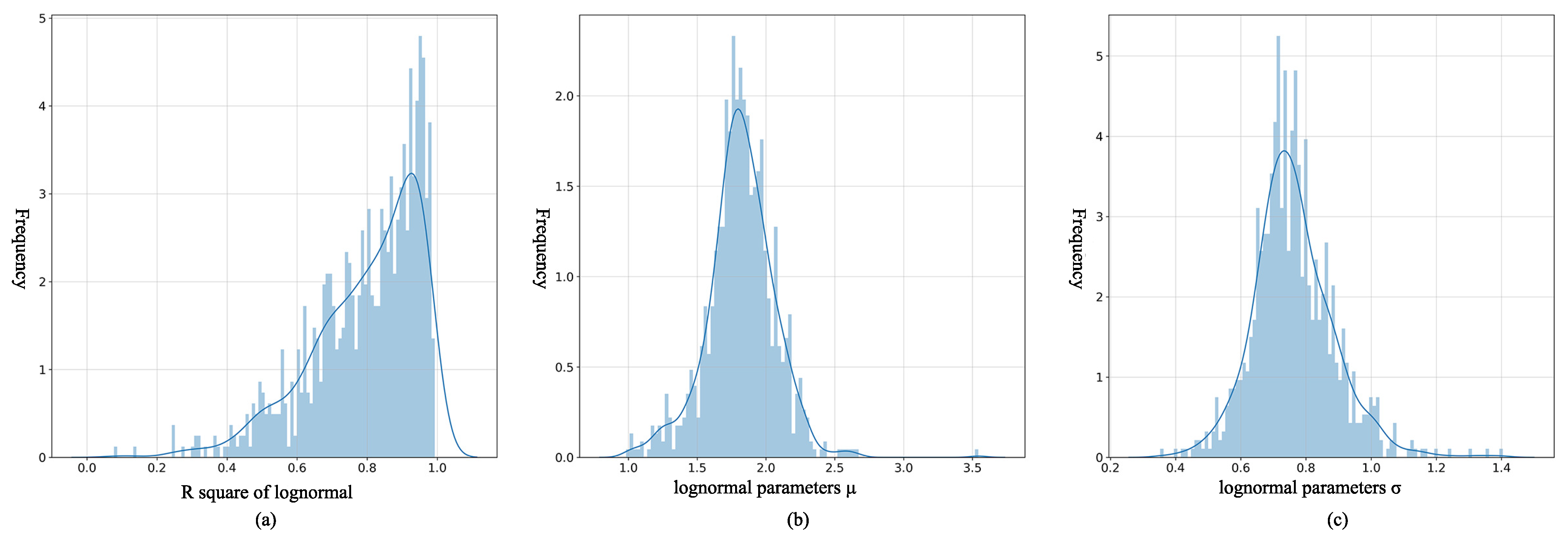
3.1.1. Best-Fit Distributions of Trip Distance

Based on the Akaike weight $w_i$, the log-normal distribution consistently outperforms the other three models in capturing travel distance patterns, fitting more than 90% of the travel distance data. Additionally, more than 85% of the nets achieve a goodness-of-fit value exceeding 0.6 (Figure 3a). The fitting parameters for the distance distribution exhibit considerable variation, indicating that the mobility characteristics of ride-hailing services are not uniform across different urban contexts within cities (Figure 3b,c).

The log-normal distribution exhibits an upward trend followed by a downward trend. The log-normal distribution has two parameters: $\mu$ and $\sigma$ (Figure 4). The parameter $\mu$ represents the highest probability point in the distribution. A smaller $\mu$ indicates that the peak of the distribution is farther to the left, indicating a smaller average travel distance. Conversely, a larger $\mu$ indicates that the peak is farther to the right, indicating a larger average travel distance. The concentration of travel is represented by $\sigma$, with a smaller $\sigma$ indicating a more concentrated trend in the graph of the log-normal distribution, meaning that travel is more concentrated, and residents’ travel activities may comprise mostly essential trips, with the proportion of non-essential activities may decreasing rapidly. A larger $\sigma$ indicates more dispersed distribution, indicating that travel is more random, with a higher proportion of decisions overcoming costs. Taking residents’ travel in the city as an example (Figure 4), smaller $\mu$ values and larger $\sigma$ values imply that residents could have relatively close average travel distances and scattered activity locations. Residents can access resources in the city relatively easily and have more choices. Larger $\mu$ values and smaller $\sigma$ values imply that residents could have farther average travel distances, and their travel activities may be mostly concentrated at specific distances, meaning that residents need to travel to specific areas to access resources.

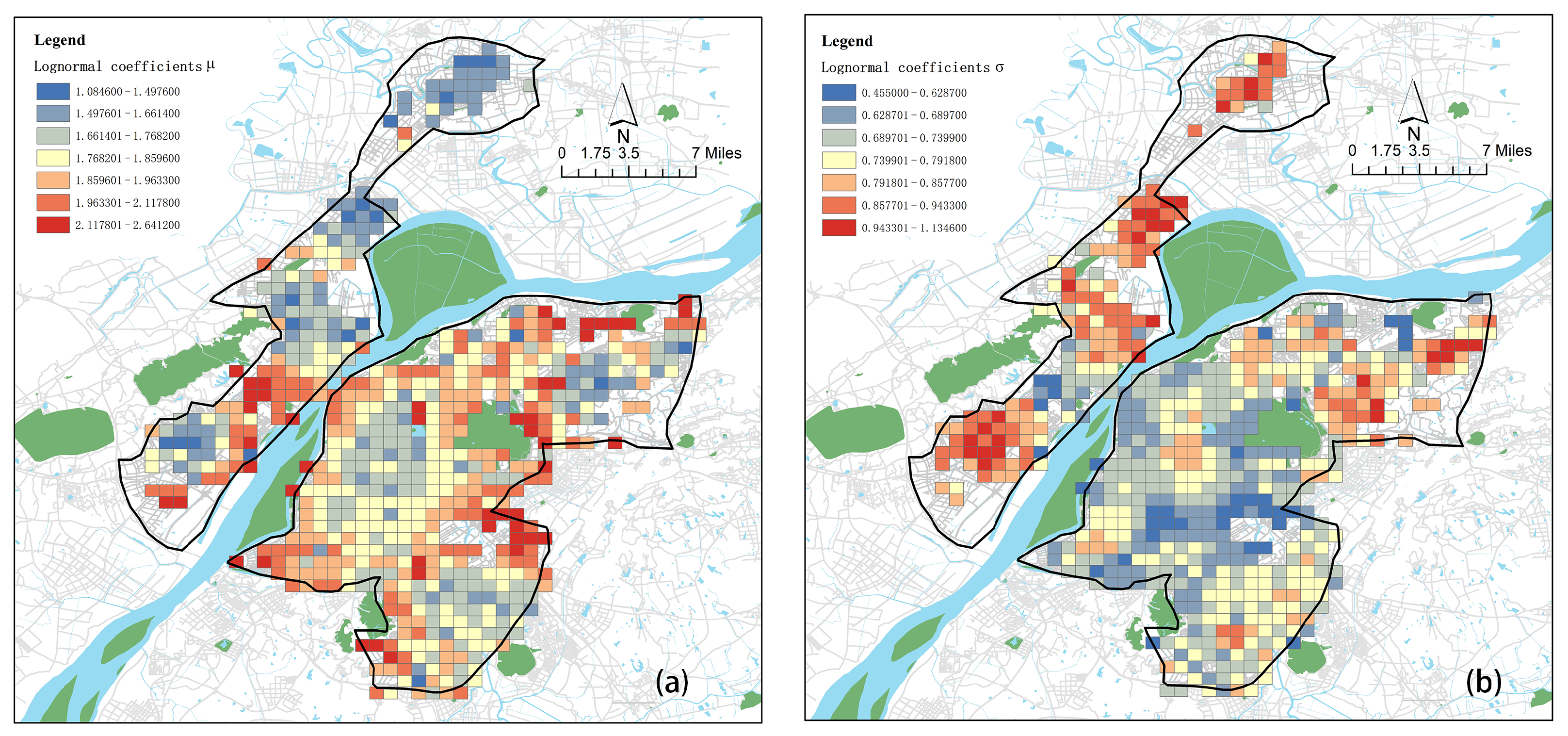
3.1.2. Spatial Distribution of Log-Normal Distribution

The spatial distribution of log-normal distribution parameters in the study area is shown in Figure 5, which demonstrates a clear gradient from the core of the city to its periphery. The parameters associated with analysis zones (nets) reveal distinct agglomeration patterns, indicating the clustering of certain characteristics or activities within specific areas. These patterns reflect the spatial concentration of urban features, which influences mobility behaviors and the distribution of services. Commercial centers, hospitals and schools in Xinjiekou, Dongshan, Xianlin, Liuhe, Dachang and Jiangbei have become the city centers of the study area. The heat map in Figure 5a shows that clusters of low-level $\mu$ values are concentrated in the city’s core areas, with the lowest category of $\mu$, ranging from 1.085 to 1.77, demarcated by blue shading.

This central area of low $\mu$ values is surrounded by a moderate-value transition zone, indicated in yellow to orange tones, reflecting a increase of 1.77 to 1.967. As we move to more marginal areas of the city, the reported incident rate rises notably, as depicted in red, indicating the highest density category of 1.967 to 2.647. Figure 5b shows that the areas north of the Yangtze River and Xianlin exhibit the highest $\sigma$ values, extending from 0.85 to 1.11. Xinjiekou, jiulonghu and tianbao display relatively high $\sigma$ values, ranging from 0.79 to 0.85. Their surrounding areas show lower $\sigma$ values that range from 0.452 to 0.79.

The model indicates a strong correlation between the parameters of the log-normal distribution and urban centrality, with the shortest distances observed in areas likely associated with high pedestrian flow and economic activity. In contrast, the city’s periphery, which may encompass housing communities and less accessible public spaces, shows longer travel distances. Interestingly, the other parameter of the log-normal distribution, $\sigma$, is roughly the opposite of $\mu$ in value. There are more travel options in the city center, resulting in a larger $\sigma$, whereas in the outskirts, the higher costs that residents need to overcome lead to a smaller $\sigma$. Intuitively, this variation might be explained by several potential differences, such as the geographical layouts of urban areas, the spatial arrangement of activity sites, and the influences of social, economic, and cultural factors.

3.2. Model Comparison

In machine learning models, the selection of adequate parameters is essential for attaining maximum efficiency. In the case of XGBoost, important parameters include n_estimators, the learning rate, max depth, min_child_weight, subsample, and gamma, all of which significantly impact model efficacy. Our tests indicated that the settings outlined in

Table 4. The optimal values for $\mu$ and $\sigma$.

	Olsample Bytree	Gamma	Learning Rate	Max Depth	n Estimators	Reg Alpha	Reg Lambda	Subsample
$\mu$	0.8	0	0.2	5	20	0	1.5	0.8
$\sigma$	1.0	0	0.2	5	30	0.1	1.5	0.8

resulted in the highest R-squared values of 0.23 and 0.41 for XGBoost, reflecting improved algorithm performance. These parameters were selected for their effectiveness in balancing model intricacy and universality. analogous optimization strategies were employed for the other models as well.

A thorough performance evaluation of the regression models, presented in

Table 5. Regression model results.

Model		R2	MAE	RMSE
OLS	$\mu$	0.13	0.14	0.18
	$\sigma$	0.27	1.07	1.09
GWR	$\mu$	0.15	1.45	0.20
	$\sigma$	0.31	1.09	0.12
RF	$\mu$	0.16	0.13	0.17
	$\sigma$	0.40	0.05	0.07
XGBoost	$\mu$	0.23	0.13	0.18
	$\sigma$	0.41	0.06	0.07

, revealed that XGBoost outperforms the OLS, GWR and RF models. XGBoost demonstrates the strongest explanatory power for the log-normal fit parameter across various networks. Furthermore, the XGBoost model demonstrates superior performance across error metrics, achieving the lowest mean absolute error (MAE) values of 0.13 and 0.06, along with root mean square error (RMSE) values of 0.18 and 0.07. These findings underscore the model’s precision and dependability in forecasting outcomes for the specified application.

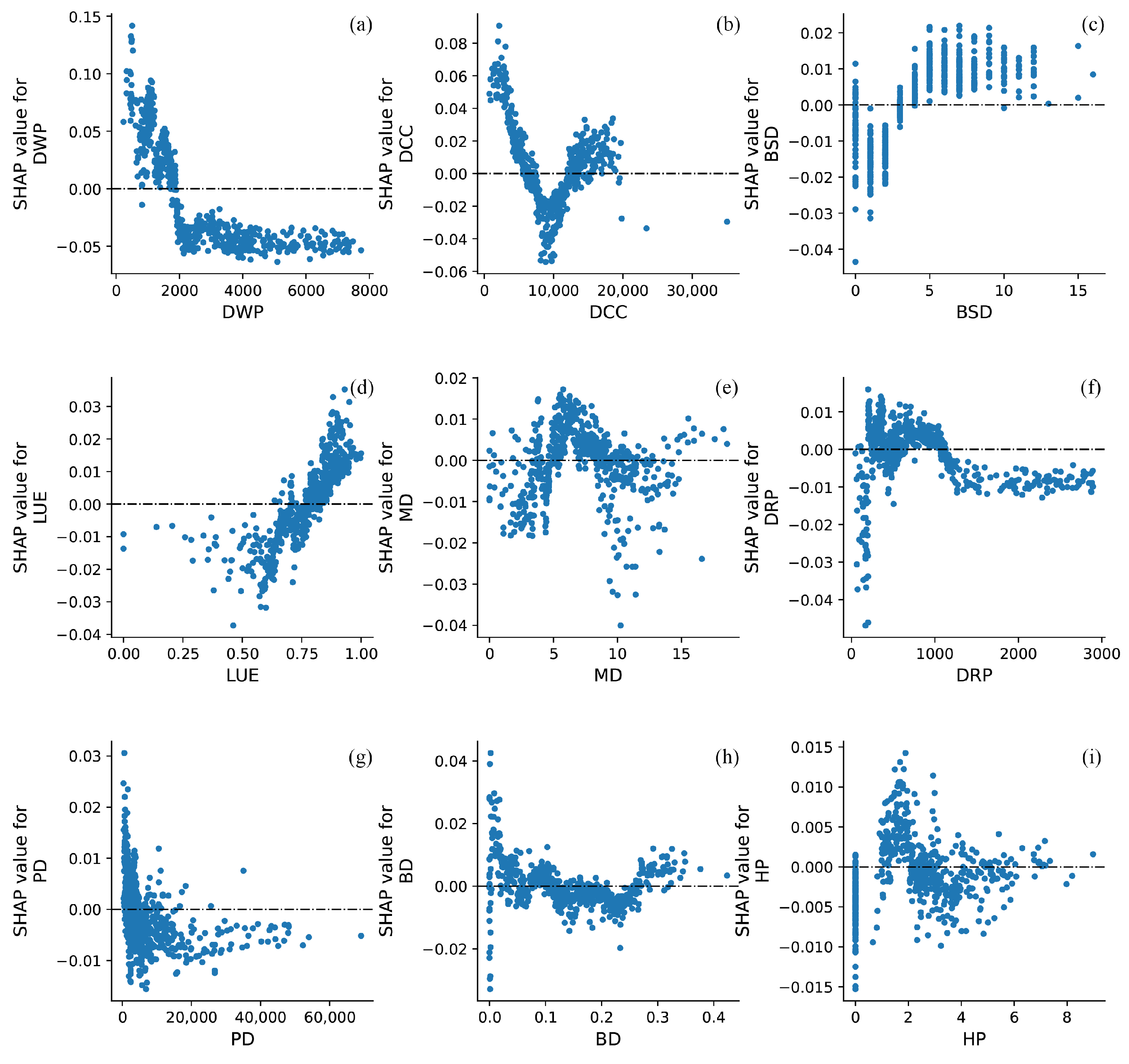
3.3. Nonlinear Relationship Interpretation Using SHAP

3.3.1. Feature Importance Analysis

To elucidate the specific urban elements that significantly predict the log-normal fit parameter, as depicted in Figure 6, the SHAP results provide a compelling representation of feature importance. In this plot, each dot represents a SHAP value linked to a specific observation, demonstrating how much each feature contributes to the model’s prediction. The dots are color-coded, where red represents higher feature values and blue signifies lower values. This color scheme effectively demonstrates the relationship between the magnitude of a feature and its influence on the model’s output. The summary chart of driving factors displays a non-uniform distribution between features with high and low values, indicating that the relationship between these crucial determinants and the log-normal fit parameters is not linear. The chart also shows the relative importance of each independent variable, indicating their respective contributions to the predictive accuracy during the modeling process, with the cumulative relative importance of all variables totaling 100%. The indicators are ranked based on their importance (

Table 6. Relative contribution of independent variables.

Category	Feature Index	Relative Marginal Contribution (%)		Ranking
		$\mu$	$\sigma$	$\mu$	$\sigma$
Socio-demographic characteristic	HP	7.06	3.85	7	9
	PD	6.85	5.12	8	7
Facility convenience	DCC	20.6	18.47	1	2
	DWP	14.25	35.25	3	1
	DRP	13.41	8.34	4	4
Construction intensity	BD	3.76	4.33	9	8
	LUE	8.52	8.26	5	5
Traffic accessibility	MD	7.66	5.91	6	6
	BSD	17.9	10.45	2	3

).

Facility convenience is the most important indicator for predicting coefficients. DCC has the greatest influence on $\mu$, reaching 20.6%. This makes sense, as commuting often constitutes the main travel activity on weekdays for a majority of individuals. The distance they commute is influenced by the locations of their residences and workplaces, with numerous employment opportunities situated in or close to urban centers. DWP has the greatest influence on $\sigma$, reaching 35.25%. The DRP has less influence than the DWP. This could be because necessary commuting is more important than non-essential commuting in urban travel concentration modes.

Construction intensity is also a key factor shaping urban mobility patterns. The role of LUE is significantly greater than that of the BD. Comparatively, the BD’s contribution to promoting resident activity is relatively limited. In particular, in large cities in which construction land is limited, the vertical expansion of construction space is more crucial than horizontal growth for internal urban activities.

Both traffic accessibility indicators play a role in shaping urban travel patterns, particularly the BSD, the relative importance of which for $\sigma$ and $\mu$ reached 17.9% and 10.45%, respectively, ranking second and third among all indicators. In Figure 5a, the right side shows an extended blue line, while the left side features a shorter red line, indicating that a low number of bus stations leads to a sharp increase in travel distances. However, a higher number of bus stations does not reduce travel distances to the same extent. Overall, the two indicators have a greater influence on $\mu$ than on $\sigma$.

Socio-economic indicators have the least impact on average trip distance and trip dispersion, ranking seventh to ninth. For $\sigma$, most HP data points are dispersed around a SHAP value of 0, indicating that this variable has little impact on the concentration of most trips. However, it is positively correlated with $\mu$.

3.3.2. Nonlinear Relationship Analysis

(1)

Driving factors of $\mu$

To investigate the cumulative influence of driving factors on $\mu$ and to quantify the relationship between these factors and $\mu$, scatter distribution charts of the SHAP values of the driving factors were generated based on the feature summary chart (Figure 7). The order of the graph is sorted by the importance of its elements.

The DCC emerges as the most influential feature in the model, exerting the greatest impact on its predictions (Figure 7a). The DCC exhibits an “N-shaped” pattern, and within the range of approximately 0 to 8000, it is negatively correlated with $\mu$. When the DCC exceeds 8000, the effect shifts from negative to positive, meaning that the farther from the city center, the larger the $\mu$ value and the longer the average travel distance. This could be due to the fact that resources are typically concentrated in city centers, so individuals living farther from the central business district tend to travel longer distances to access various resources [44].

When the BSD exceeds 4, the impact shifts from positive to negative (Figure 7b). In areas with a higher density of bus stations, residents may be more likely to opt for other modes of transportation to meet long-distance travel needs, while ride-hailing is more often used to supplement short-distance connections. The analysis further indicates that a rivalry between short-distance ride-hailing options and public transit in the central urban zones [45]. The nonlinear impact of bus station density likely reflects a saturation point at which additional stations no longer significantly improve travel distances.

The DRP positively influences $\mu$ at around 100 and negatively influences $\mu$ at around 200 (Figure 7c). An excess of entertainment facilities (exceeding 1000) negative affects the average trip distance of ride-hailing services. First, most entertainment needs, such as movies, dining, or exercise facilities, are localized, meaning that residents tend to choose facilities close to home rather than traveling long distances across regions. Additionally, areas with a high density of entertainment facilities often have a well-developed transportation infrastructure, enabling people to opt for public transportation, bicycling or walking instead of relying on long-distance ride-hailing services.

When the DWP exceeds 4800, it is negatively correlated with $\mu$ (Figure 7d). This indicates that increasing the number of companies beyond this threshold may reduce the commuting distance for ride-hailing services used for work. The increase in workplace facilities enhances the likelihood of residents finding jobs nearby, particularly in densely populated residential communities. This reduces the need for long-distance commuting to meet employment needs.

We observed that the impact of LUE on $\mu$ shifts from positive to negative around 0.75 (Figure 7e). After 0.9, the higher the LUE, the longer the travel distance. We note that the nonlinear influence of land use entropy may stem from threshold effects in which a balanced mix of land uses promotes efficient mobility but excessive diversity could lead to congestion or inefficiency.

When the MD is below approximately 4, it is positively correlated with $\mu$. This may be because certain residential communities, scenic areas or campuses, despite having low road density, can generate a significant amount of long-distance travel. The MD shows a correlation with distance traveled, and SHAP values tend to be positive as motor vehicle lanes increase to 8.5 (Figure 7g). The denser the motorized lanes, the more convenient it is to travel via car and the more likely it is that long-distance trips are made.

When the HP exceeds 20,000 (Figure 7h), it positively influences the average travel distance. This may be because residents in high-priced areas have greater financial capacity, allowing for a wider range of activities and travel.

When the BD exceeds 0.25, it negatively impacts $\mu$. This is likely because areas with high building density are often equipped with more living and working facilities (e.g., commercial, office, entertainment), reducing the need for long-distance travel. Most points for the PD are distributed near zero, suggesting that its impact on $\mu$ may be minimal. This could be because population size primarily influences the total travel demand rather than the travel distance. In other words, a larger population increases the number of ride-hailing orders but does not directly alter the length of trips.

(2)

Driving factors of $\sigma$

Figure 8 presents nonlinear relationships between the log-normal fit parameter $\sigma$ and built environment variables.

When the DWP reaches 2000, its effect on $\sigma$ shifts from positive to negative and stabilizes (Figure 8a). However, as the DWP reaches 3000, the local effect remains at its lowest value, indicating that beyond a certain threshold, increasing the number of companies does not further enhance the dispersion of travel distances. The increase in the number of companies is often associated with improved job-housing balance, allowing more people to find employment near their residences. In such cases, travel distances tend to stabilize, and ride-hailing trip lengths do not diversify further as the number of companies grows.

The DCC is positively correlated with the log-normal fit parameter $\sigma$ for distances less than 5000 m or greater than 13,000 m (Figure 8b). This may be due to the fact that some residents start from the city center, from which there are many ride-hailing rides with a high dispersion of distance distribution, while some residents start from sub-centers more than 13 km from the city center, with a higher dispersion of distance distribution for their trips.

When the BSD is between 0 and 4, it is negatively correlated with $\sigma$ (Figure 8c). This may be because in suburban areas with limited bus availability, ride-hailing serves as a complementary mode of transportation to public transit. The fewer the buses, the greater the diversity in ride-hailing trips. In areas with fewer buses, passengers rely more heavily on ride-hailing services as public transit routes cannot meet their travel needs. Whether for short distances (e.g., shopping, last-mile connections) or long distances (e.g., cross-district commutes, suburban outings), passengers tend to choose ride-hailing services and taxis, leading to greater diversity in travel distances. After the BSD exceeds 4, the trend changes, and the BSD value positively affects the dispersion. This indicates that areas in the city center have many bus stations and ride-hailing services, leading to a more dispersed distribution of travel distances.

The trend changes when the mixing degree is greater than 0.75 (Figure 8d). The LUE value initially has a negative effect on dispersion, indicating that in areas with lower levels of facility mixing, residents’ travel distances tend to be more concentrated, suggesting that insufficient functional diversity hinders travel diversity. However, beyond this threshold, the effect of mixing degree shifts to a positive value. Areas with high LUE typically feature a combination of functions such as residential, commercial, office, entertainment, and public services. This multifunctional overlap diversifies travel purposes and destinations, leading to a high degree of variability in travel distances. Additionally, regions with high LUE often attract not only local residents but also a significant transient population (e.g., commuters and tourists), further increasing the diversity of travel distances within the area.

When the MD is less than 5 or greater than 8, it negatively impacts the SHAP (Figure 8e), indicating that both very low and very high motor vehicle lane densities are not conducive to promoting travel diversity. In areas with excessively low road density, land is often allocated to single-use functions (e.g., residential or agricultural) lacking the mixed-use features of commercial, office or entertainment spaces. This functional singularity forces residents to travel across regions for daily needs such as work, shopping and leisure, concentrating travel patterns on fixed long-distance commuting. what’s more, an excessively high road density implies a tightly knit road network in which distances between destinations are shortened. In such areas, residents tend to walk, cycle or use shared transportation for short-distance travel. Consequently, ride-hailing orders could be limited primarily to short-distance trips (e.g., from residential areas to the nearest subway station), resulting in a significant reduction in long-distance ride-hailing demand.

When the DRP is between 250 and 1100, it positively influences travel dispersion (Figure 8f), meaning that the greater number of recreational facilities there are available, the greater the dispersion of trips. When the DRP is less than 250, residents have fewer entertainment options, leading to more concentrated travel patterns. When the DRP exceeds 1100, The local effect tends to stabilize. When the number of nearby entertainment facilities increases to a certain threshold, residents tend to choose closer facilities rather than distant ones. As a result, even with an increase in the number of entertainment facilities, the distribution of travel distances does not change significantly and may become more concentrated within a short-distance range.

When the PD (Figure 8g) exceeds 10,000, its local effect shifts from positive to negative. However, as the PD reaches 20,000, the local effect stabilizes at its minimum value, indicating that beyond a certain threshold, the influence of the PD on $\sigma$ does not continue to increase. The effect of the BD (Figure 8h) and HP(Figure 8i) on SHAP tends to be close to zero, suggesting that there may not be a direct relationship between the distribution of distance traveled on ride-hailing trips and the distribution of the BD and HP.

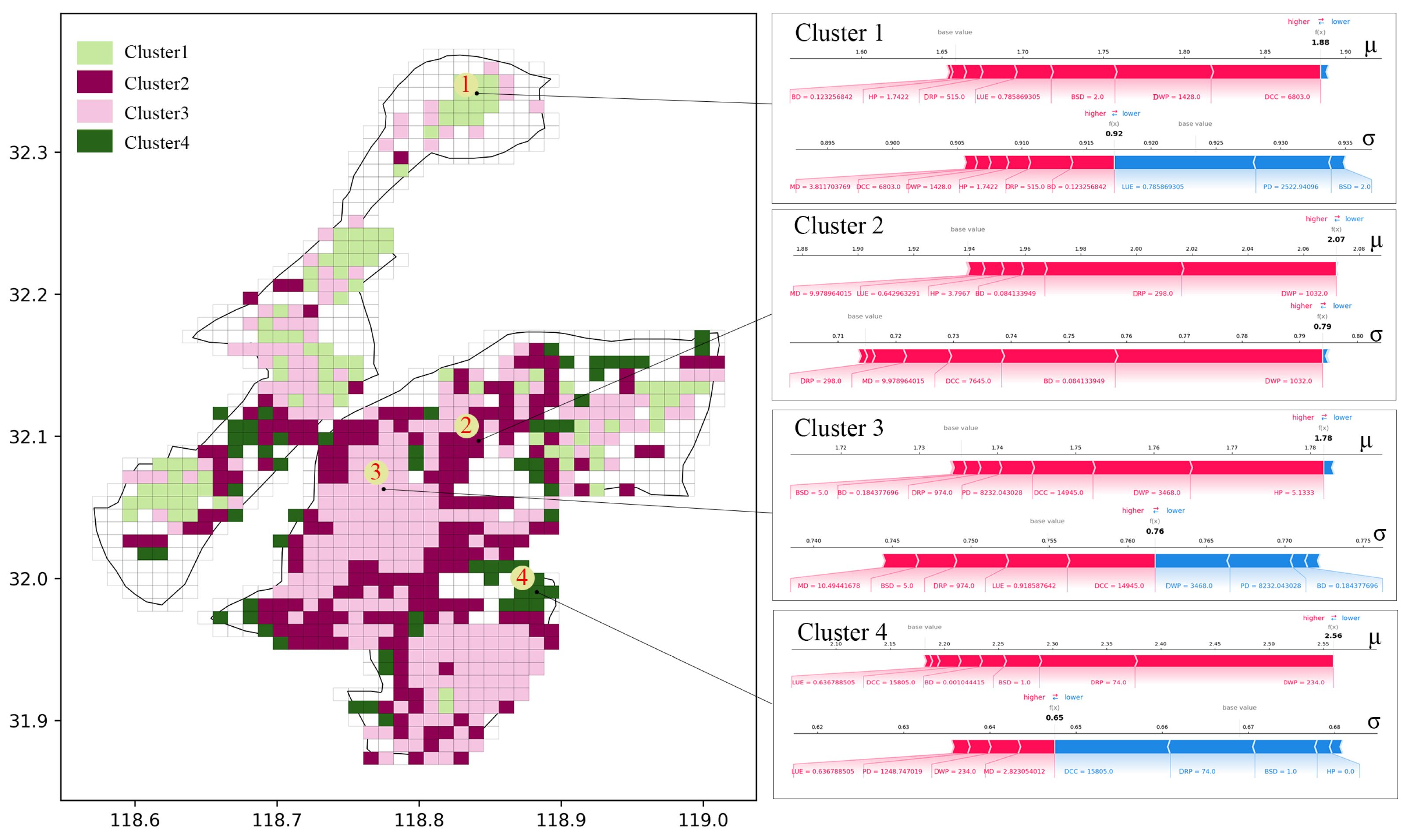
3.3.3. Local and Spatial Effects on Coefficients

A clustering approach was employed to categorize grids exhibiting similar patterns of local effects. This method enables the identification of spatially coherent regions in which driving factors influence outcomes in comparable ways, facilitating a more nuanced understanding of localized urban dynamics. Figure 9 graphically displays the local explanations for four chosen grids within the study area, each symbolizing different clusters. As shown in Figure 9, four types of travel patterns were identified, accounting for 15%, 30%, 45% and 10%, respectively. The red and blue bar charts in Figure 9 represent the local impact effects of the travel patterns, with red signifying positive variables and blue signifying negative variables. The boundary between the red and blue bars represents the predicted values for $\sigma$ and $\mu$.

Cluster 1 shows a smaller $\mu$ and a larger $\sigma$. In this case, the case 1 is situated at Wanda Plaza in Liuhe. The geographic barrier created by the river separating the city’s sub-center from the main urban area limits travel demand on the opposite bank to within the local region. Within the sub-center, short-distance trips, such as shopping and dining, dominate. In contrast, outbound (cross-river) commuting or visitor flows may require medium-distance travel. This dual demand leads to a diversification of travel distances. Factors such as the DCC, DWP, BSD, LUE, DRP, HP, and BD positively influence the average ride-hailing trip distance. Additionally, the LUE, PD, and BSD all contribute to decreasing trip dispersion.

Class 2 shows a larger $\mu$ and a medium $\sigma$. The second case is situated in Nanjing’s residential district, Yingtiecun Community, which is on the south side of Xuanwu Avenue. Factors such as the DWP, DRP, BD, HP, LUE and MD all have a significant positive influence on the average ride-hailing trip distance, suggesting that areas with higher values for these features tend to require longer travel distances. Additionally, the NWP, BD, DCC, MD and DRP positively influence the dispersion of ride-hailing trips, indicating that these factors contribute to greater diversity in trip destinations and routes, thereby increasing travel dispersion.

Class 3 exhibits the smallest $\mu$ and a moderate $\sigma$, representing a well-developed and mature urban area with higher housing prices and more job opportunities. Case 3, which is located in Xinjiekou near the Nanjing World Trade Center, features high functional density, allowing residents and visitors to meet most of their travel needs within a compact area. This leads to shorter ride-hailing distances while supporting a diverse range of trips, reflecting a wide distribution of destinations across the city. Key features such as the HP, NWP, DCC, PD, NRP, BD, and BSD positively influence the average ride-hailing trip distance. Meanwhile, the MD, BSD, NRP, LUE, and DCC positively affect trip dispersion, whereas the NWP, PD, and BD have a negative impact on trip dispersion.

Cluster 4, which is located on the outskirts of the city, has the largest $\mu$ and the smallest $\sigma$, as seen in case 4. The ride-hailing distances are longer, but the diversity of trip distances is lower. This may be due to the functional singularity of peripheral areas, which results in a concentration of travel destinations; insufficient public transportation and sparse road networks, which limit travel options; and job–housing separation, which may lead to long-distance commuting dominating the travel demand. Features such as the DWP, DRP, BSD, BD, DCC, and LUE positively influence the average ride-hailing trip distance. However, the DCC, DRP, BSD, and HP reduce trip dispersion.

4. Discussion

4.1. Comprehensive Interpretation of Nonlinear Relationships

This study provides a comprehensive analysis of urban mobility patterns based on ride-hailing data collected for Nanjing, China. Key findings include the quantification of travel distances using probability density functions (PDFs) derived from ride-hailing trip data, revealing significant spatial heterogeneity. The results also highlight the nonlinear and threshold effects of explanatory variables, such as land use entropy and bus station density, on the distribution of travel distances. These results highlight the significance of accounting for spatial and contextual differences when modeling urban mobility patterns.

The analysis highlights how urban mobility patterns are influenced by built environment factors through nonlinear and threshold effects. (1) DCC: Travel distances ($\mu$) decrease up to 8000 m and then increase as individuals travel farther to access resources [35]. Variability ($\sigma$) is higher close to urban cores and sub-centers [46]. (2) BSD: Beyond four stations, the BSD reduces travel distances ($\mu$) as residents rely more on walking or cycling [47]. The presence of a few stations decreases dispersion ($\sigma$), while many stations diversify urban trips. (3) DWP: A higher density (above 4800) reduces commuting distances ($\mu$) by improving the job–housing balance [6,48]. Travel dispersion ($\sigma$) stabilizes beyond 2000 companies. (4) DRP: A moderate recreational facility density increases travel dispersion ($\sigma$) and supports longer travel distances ($\mu$). However, as the facility density surpasses a threshold (approximately 1100), residents increasingly choose closer facilities, stabilizing travel distances and reducing variability [49]. (5) LUE: Balanced land use shortens trips ($\mu$), while excessive diversity increases travel inefficiencies and dispersion ($\sigma$) [50]. (6) MD: Denser motorized lanes (up to 8.5) facilitate longer trips ($\mu$). Extremely low or high densities limit travel diversity ($\sigma$). (7) HP: Higher-priced areas correlate with longer travel distances ($\mu$) [51]. The impact on dispersion ($\sigma$) is minimal. (8) BD: High building density reduces long-distance travel ($\mu$) as it supports localized living and working facilities. This concentration of facilities minimizes the need for dispersed trips, making its impact on travel dispersion ($\sigma$) negligible. (9) PD: A higher population density primarily increases the total demand for travel [33], without significantly altering travel distances ($\mu$). Dispersion ($\sigma$) decreases beyond a threshold (20,000).

4.2. Policy Implications

The average length and dispersion of travel distances can be influenced by maintaining built environment elements within appropriate ranges; the following approaches may be used: (1) Promoting the job–housing balance—balancing the distribution of workplaces and residential areas within urban regions to reduce long-distance commuting demands; when DWP is greater than 4800 and DRP is greater than 800, both factors suppress $\mu$. (2) Adjusting LUE to an appropriate level—promoting urban functional diversity by increasing the availability of commercial, educational, medical and entertainment facilities around residential areas. When LUE is between 0.75 and 0.85, it reduces the demand for cross-regional long-distance ride-hailing caused by single-function land distribution. Such planning helps allocate urban resources more effectively, optimize residents’ travel patterns and foster sustainable urban development. (3) Optimizing the public transportation network layout—increasing bus routes in low-coverage areas, particularly rapid transit lines connecting suburban areas to the city center. In areas where BSD exceeds 4, residents are less likely to rely on ride-hailing for long-distance commuting. (4) Enhancing connections with public transportation—establishing ride-hailing pick-up points at key nodes such as subway stations and bus hubs to facilitate short-distance transfers. This approach will increase the number of short-distance ride-hailing trips and enhance the diversity of travel distances. (5) Encouraging the transition of short-distance ride-hailing in urban centers to sustainable modes of transportation. It is worthwhile to encourage the transition of short-distance ride-hailing to sustainable modes of transportation, especially during peak hours [52]. Specifically, enhancing public transit subsidies are effective strategies. Moreover, raising the cost of short-distance ride-hailing during peak periods and rationalizing free-floating bike-sharing systems can motivate non-urgent short-trip travelers to opt for walking or public transportation.

4.3. Limitations and Future Directions

Due to data limitations, we were unable to incorporate a sufficient range of socio-economic characteristics across different regions. Nevertheless, it is expected that socio-economic factors could significantly effect the distance distribution patterns. For example, variations in income may affect travel behaviors, while different age groups and gender identities might lead to distinct mobility choices. Furthermore, our empirical analysis was limited to an online car-hailing dataset exclusively from Nanjing, China, which may restrict the applicability of our findings to other urban contexts. The reliance on ride-hailing data may introduce biases, as these datasets predominantly capture certain demographic or geographic user groups, potentially leading to an incomplete representation of urban mobility patterns. Urban mobility patterns are inherently variable due to temporal, spatial and socio-economic factors. The current study does not extensively discuss how this variability might impact the robustness of the results. Future studies should aim to incorporate a broader range of socio-economic indicators and diverse datasets from multiple locations to deepen the understanding of these relationships. Additionally, integrating alternative data sources, such as public transit or pedestrian movement data, could improve the generalizability of the findings. To further enhance the robustness of the results, future research could also perform sensitivity analyses to evaluate the stability of the conclusions under varying scenarios.

5. Conclusions

The best-fit distributions of trip distance with its parameters were first shown. Then, we further analyzed the nonlinear relationship interpretation and interaction effects of the built environment. Finally, we attempted to identify the local and spatial effects on human mobility.

Over the past decade, a surge of technological advancements has significantly increased the interest of researchers and urban planners in ride-hailing services. However, related performance, usage patterns, and interactions with the built environment remain underexplored. This research, based on empirical data from Nanjing, China, aimed to fill a gap in existing literature by analyzing the spatial variability in the distribution of distances in online car-hailing and its nonlinear interactions with the built environment. The objective was to comprehend how ride-hailing spatially interacts within urban contexts, thereby guiding sustainable urban planning and encouraging broader adoption of these services in various urban environments.

Distance distribution functions for various regions were estimated using 1 × 1 km analysis zones. The optimal model was chosen to empirically assess these functions across different areas. Our analysis uncovered significant spatial heterogeneity in the distance distribution of online car-hailing usage across diverse urban environments. By utilizing data from varied sources, we identified multiple built environmental factors—including facility convenience, construction intensity, traffic accessibility, and socio-demographic characteristics—within different research units. We employed the XGBoost model to explore the nonlinear relationships between these built environment factors and the log-normal fit parameters of online car-hailing. Our findings demonstrate that certain built environment factors significantly influence the distance distribution laws governing online car-hailing trips. Regarding $\mu$, the BSD and LUM negatively affected $\mu$, while the DCC and DWP positively affected $\mu$. As for $\sigma$, the BSD and LUM both positively affected $\sigma$, while the DWP, DCC, and BD negatively affected $\sigma$. Furthermore, the use of SHAP enhanced our understanding of the nonlinear relationships by elucidating how the variables interact with the log-normal fit parameters. This method allowed for a more detailed analysis of the contributions of each variable to the model’s predictions.

The primary contributions and key findings of this study are outlined as follows: First, this study identified the significant influence of built environment and socio-economic factors on urban mobility patterns. Second, the application of advanced machine learning techniques, such as XGBoost and SHAP, enhanced the interpretability of model outcomes. Third, this study offers policy-relevant insights by linking urban design elements with mobility behaviors, providing a foundation for sustainable urban planning strategies tailored to specific city contexts.

References

1. Gonzalez, M.C.; Hidalgo, C.A.; Barabasi, A.L. Understanding individual human mobility patterns. Nature 2008, 453, 779–782. [Google Scholar] [CrossRef] [PubMed]
2. Jiang, B.; Yin, J.; Zhao, S. Characterizing the human mobility pattern in a large street network. Phys. Rev. E-Stat. Nonlinear Soft Matter Phys. 2009, 80, 021136. [Google Scholar] [CrossRef] [PubMed]
3. Ratti, C.; Frenchman, D.; Pulselli, R.M.; Williams, S. Mobile landscapes: Using location data from cell phones for urban analysis. Environ. Plan. B Plan. Des. 2006, 33, 727–748. [Google Scholar] [CrossRef]
4. Liu, H.; Chen, Y.H.; Lih, J.S. Crossover from exponential to power-law scaling for human mobility pattern in urban, suburban and rural areas. Eur. Phys. J. B 2015, 88, 1–7. [Google Scholar] [CrossRef]
5. Alessandretti, L.; Sapiezynski, P.; Lehmann, S.; Baronchelli, A. Multi-scale spatio-temporal analysis of human mobility. PLoS ONE 2017, 12, e0171686. [Google Scholar] [CrossRef]
6. Zheng, Z.; Zhou, S.; Deng, X. Exploring both home-based and work-based jobs-housing balance by distance decay effect. J. Transp. Geogr. 2021, 93, 103043. [Google Scholar] [CrossRef]
7. Blondel, V.D.; Decuyper, A.; Krings, G. A survey of results on mobile phone datasets analysis. EPJ Data Sci. 2015, 4, 1–55. [Google Scholar] [CrossRef]
8. Brockmann, D.; Hufnagel, L.; Geisel, T. The scaling laws of human travel. Nature 2006, 439, 462–465. [Google Scholar] [CrossRef] [PubMed]
9. Liang, X.; Zheng, X.; Lv, W.; Zhu, T.; Xu, K. The scaling of human mobility by taxis is exponential. Phys. A Stat. Mech. Appl. 2012, 391, 2135–2144. [Google Scholar] [CrossRef]
10. Bazzani, A.; Giorgini, B.; Rambaldi, S.; Gallotti, R.; Giovannini, L. Statistical laws in urban mobility from microscopic GPS data in the area of Florence. J. Stat. Mech. Theory Exp. 2010, 2010, P05001. [Google Scholar] [CrossRef]
11. Riccardo, G.; Armando, B.; Sandro, R. Towards a statistical physics of human mobility. Int. J. Mod. Phys. C 2012, 23, 1250061. [Google Scholar] [CrossRef]
12. Jurdak, R.; Zhao, K.; Liu, J.; AbouJaoude, M.; Cameron, M.; Newth, D. Understanding human mobility from Twitter. PLoS ONE 2015, 10, e0131469. [Google Scholar] [CrossRef] [PubMed]
13. Liu, Y.; Sui, Z.; Kang, C.; Gao, Y. Uncovering patterns of inter-urban trip and spatial interaction from social media check-in data. PLoS ONE 2014, 9, e86026. [Google Scholar] [CrossRef] [PubMed]
14. Wu, L.; Zhi, Y.; Sui, Z.; Liu, Y. Intra-urban human mobility and activity transition: Evidence from social media check-in data. PLoS ONE 2014, 9, e97010. [Google Scholar] [CrossRef] [PubMed]
15. Gong, L.; Liu, X.; Wu, L.; Liu, Y. Inferring trip purposes and uncovering travel patterns from taxi trajectory data. Cartogr. Geogr. Inf. Sci. 2016, 43, 103–114. [Google Scholar] [CrossRef]
16. Wang, W.; Pan, L.; Yuan, N.; Zhang, S.; Liu, D. A comparative analysis of intra-city human mobility by taxi. Phys. A Stat. Mech. Appl. 2015, 420, 134–147. [Google Scholar] [CrossRef]
17. Tang, J.; Liu, F.; Wang, Y.; Wang, H. Uncovering urban human mobility from large scale taxi GPS data. Phys. A Stat. Mech. Appl. 2015, 438, 140–153. [Google Scholar] [CrossRef]
18. Shi, C.; Li, Q.; Lu, S.; Yang, X. Exploring temporal intra-urban travel patterns: An online car-hailing trajectory data perspective. Remote Sens. 2021, 13, 1825. [Google Scholar] [CrossRef]
19. Shi, C.; Li, Q.; Lu, S.; Yang, X. Modeling the Distribution of Human Mobility Metrics with Online Car-Hailing Data—An Empirical Study in Xi’an, China. ISPRS Int. J. Geo-Inf. 2021, 10, 268. [Google Scholar] [CrossRef]
20. Chai, Y. Space–time behavior research in China: Recent development and future prospect: Space–time integration in geography and GIScience. Ann. Assoc. Am. Geogr. 2013, 103, 1093–1099. [Google Scholar] [CrossRef]
21. Cheng, L.; Chen, X.; Yang, S.; Cao, Z.; De Vos, J.; Witlox, F. Active travel for active ageing in China: The role of built environment. J. Transp. Geogr. 2019, 76, 142–152. [Google Scholar] [CrossRef]
22. Wang, D.; Zhou, M. The built environment and travel behavior in urban China: A literature review. Transp. Res. Part D Transp. Environ. 2017, 52, 574–585. [Google Scholar] [CrossRef]
23. Dong, W.; Wang, S.; Liu, Y. Mapping relationships between mobile phone call activity and regional function using self-organizing map. Comput. Environ. Urban Syst. 2021, 87, 101624. [Google Scholar] [CrossRef]
24. Tu, W.; Zhu, T.; Xia, J.; Zhou, Y.; Lai, Y.; Jiang, J.; Li, Q. Portraying the spatial dynamics of urban vibrancy using multisource urban big data. Comput. Environ. Urban Syst. 2020, 80, 101428. [Google Scholar] [CrossRef]
25. Yang, X.; Fang, Z.; Xu, Y.; Yin, L.; Li, J.; Lu, S. Spatial heterogeneity in spatial interaction of human movements—Insights from large-scale mobile positioning data. J. Transp. Geogr. 2019, 78, 29–40. [Google Scholar] [CrossRef]
26. Cheng, L.; De Vos, J.; Zhao, P.; Yang, M.; Witlox, F. Examining non-linear built environment effects on elderly’s walking: A random forest approach. Transp. Res. Part D Transp. Environ. 2020, 88, 102552. [Google Scholar] [CrossRef]
27. Friedman, J.H. Greedy function approximation: A gradient boosting machine. Ann. Stat. 2001, 29, 1189–1232. [Google Scholar] [CrossRef]
28. Yang, X.; Li, J.; Fang, Z.; Chen, H.; Li, J.; Zhao, Z. Influence of residential built environment on human mobility in Xining: A mobile phone data perspective. Travel Behav. Soc. 2024, 34, 100665. [Google Scholar] [CrossRef]
29. Shaheen, S.; Bell, C.; Cohen, A.; Yelchuru, B. Travel Behavior: Shared Mobility and Transportation Equity; Technical Report; United States Federal Highway Administration, Office of Policy & Governmental Affairs: Washington, DC, USA, 2017.
30. Zhang, B.; Chen, S.; Ma, Y.; Li, T.; Tang, K. Analysis on spatiotemporal urban mobility based on online car-hailing data. J. Transp. Geogr. 2020, 82, 102568. [Google Scholar] [CrossRef]
31. Šveda, M.; Madajová, M.S. Estimating distance decay of intra-urban trips using mobile phone data: The case of Bratislava, Slovakia. J. Transp. Geogr. 2023, 107, 103552. [Google Scholar] [CrossRef]
32. Wagenmakers, E.J.; Farrell, S. AIC model selection using Akaike weights. Psychon. Bull. Rev. 2004, 11, 192–196. [Google Scholar] [CrossRef] [PubMed]
33. Wang, S.; Noland, R.B. Variation in ride-hailing trips in Chengdu, China. Transp. Res. Part D Transp. Environ. 2021, 90, 102596. [Google Scholar] [CrossRef]
34. Zheng, Z.; Zhang, J.; Zhang, L.; Li, M.; Rong, P.; Qin, Y. Understanding the impact of the built environment on ride-hailing from a spatio-temporal perspective: A fine-scale empirical study from China. Cities 2022, 126, 103706. [Google Scholar] [CrossRef]
35. Ding, C.; Cao, X.J.; Næss, P. Applying gradient boosting decision trees to examine non-linear effects of the built environment on driving distance in Oslo. Transp. Res. Part A Policy Pract. 2018, 110, 107–117. [Google Scholar] [CrossRef]
36. Zhao, P.; Xu, Y.; Liu, X.; Kwan, M.P. Space-time dynamics of cab drivers’ stay behaviors and their relationships with built environment characteristics. Cities 2020, 101, 102689. [Google Scholar] [CrossRef]
37. Gao, K.; Yang, Y.; Li, A.; Qu, X. Spatial heterogeneity in distance decay of using bike sharing: An empirical large-scale analysis in Shanghai. Transp. Res. Part D Transp. Environ. 2021, 94, 102814. [Google Scholar] [CrossRef]
38. Xu, Y.; Yan, X.; Liu, X.; Zhao, X. Identifying key factors associated with ridesplitting adoption rate and modeling their nonlinear relationships. Transp. Res. Part A Policy Pract. 2021, 144, 170–188. [Google Scholar] [CrossRef]
39. Yi, S.; Li, X.; Wang, R.; Guo, Z.; Dong, X.; Liu, Y.; Xu, Q. Interpretable spatial machine learning insights into urban sanitation challenges: A case study of human feces distribution in San Francisco. Sustain. Cities Soc. 2024, 113, 105695. [Google Scholar] [CrossRef]
40. Luo, Y.; Yan, J.; McClure, S. Distribution of the environmental and socioeconomic risk factors on COVID-19 death rate across continental USA: A spatial nonlinear analysis. Environ. Sci. Pollut. Res. 2021, 28, 6587–6599. [Google Scholar] [CrossRef] [PubMed]
41. Grekousis, G.; Feng, Z.; Marakakis, I.; Lu, Y.; Wang, R. Ranking the importance of demographic, socioeconomic, and underlying health factors on US COVID-19 deaths: A geographical random forest approach. Health Place 2022, 74, 102744. [Google Scholar] [CrossRef]
42. Doan, Q.C.; Ma, J.; Chen, S.; Zhang, X. Nonlinear and threshold effects of the built environment, road vehicles and air pollution on urban vitality. Landsc. Urban Plan. 2025, 253, 105204. [Google Scholar] [CrossRef]
43. Li, Z. Extracting spatial effects from machine learning model using local interpretation method: An example of SHAP and XGBoost. Comput. Environ. Urban Syst. 2022, 96, 101845. [Google Scholar] [CrossRef]
44. Tu, M.; Li, W.; Orfila, O.; Li, Y.; Gruyer, D. Exploring nonlinear effects of the built environment on ridesplitting: Evidence from Chengdu. Transp. Res. Part D Transp. Environ. 2021, 93, 102776. [Google Scholar] [CrossRef]
45. Li, X.; Xu, J.; Du, M.; Liu, D.; Kwan, M.P. Understanding the spatiotemporal variation of ride-hailing orders under different travel distances. Travel Behav. Soc. 2023, 32, 100581. [Google Scholar] [CrossRef]
46. Stead, D.; Marshall, S. The relationships between urban form and travel patterns. An international review and evaluation. Eur. J. Transp. Infrastruct. Res. 2001, 1. [Google Scholar] [CrossRef]
47. Cao, Y.; Jiang, D.; Wang, S. Optimization for feeder bus route model design with station transfer. Sustainability 2022, 14, 2780. [Google Scholar] [CrossRef]
48. Suzuki, T.; Lee, S. Jobs–housing imbalance, spatial correlation, and excess commuting. Transp. Res. Part A Policy Pract. 2012, 46, 322–336. [Google Scholar] [CrossRef]
49. Cheng, C.C.; Wu, H.C.; Tsai, M.C.; Chang, Y.Y.; Chen, C.T. Determinants of customers’ choice of dining-related services: The case of Taipei City. Br. Food J. 2020, 122, 1549–1571. [Google Scholar] [CrossRef]
50. Kanyepe, J.; Tukuta, M.; Chirisa, I. Urban land-use and traffic congestion: Mapping the interaction. J. Contemp. Urban Aff. 2021, 5, 77–84. [Google Scholar] [CrossRef]
51. Xu, Y.; Belyi, A.; Bojic, I.; Ratti, C. Human mobility and socioeconomic status: Analysis of Singapore and Boston. Comput. Environ. Urban Syst. 2018, 72, 51–67. [Google Scholar] [CrossRef]
52. Meredith-Karam, P.; Kong, H.; Wang, S.; Zhao, J. The relationship between ridehailing and public transit in Chicago: A comparison before and after COVID-19. J. Transp. Geogr. 2021, 97, 103219. [Google Scholar] [CrossRef]
Figure 1. Research framework.
Ijgi 14 00039 g001
Figure 2. Study area.
Ijgi 14 00039 g002
Figure 3. Frequency histograms of R square, μ and σ . (a) R square of lognormal functions. (b) The distribution of the lognormal parameter μ . (c) The distribution of the lognormal parameter σ (The blue line likely represents a fitted probability density function).
Ijgi 14 00039 g003
Figure 4. Log-normal distribution diagram.
Ijgi 14 00039 g004
Figure 5. Spatial distribution of log-normal distribution. (a) The coefficients μ of log-normal distribution in urban space. (b) The coefficients σ of log-normal distribution in urban space.
Ijgi 14 00039 g005
Figure 6. Feature importance. (a) Findings of SHAP feature importance analysis of log-normal fit parameter μ ; (b) Findings of SHAP feature importance analysis of log-normal fit parameter σ .
Ijgi 14 00039 g006
Figure 7. Nonlinear relationships between log-normal fit parameter μ and variables. (a) DCC; (b) BSD; (c) DRP; (d) DWP; (e) LUE; (f) PD; (g) MD; (h) HP; (i) BD.
Ijgi 14 00039 g007
Figure 8. Nonlinear relationships between log-normal fit parameter σ and variables. (a) DWP; (b) DCC; (c) BSD; (d) LUE; (e) MD; (f) DRP; (g) PD; (h) BD; (i) HP.
Ijgi 14 00039 g008
Figure 9. Clustered SHAP value and local effects by cluster type.
Ijgi 14 00039 g009