


Unraveling Spatial Nonstationary and Nonlinear Dynamics in Life Satisfaction: Integrating Geospatial Analysis of Community Built Environment and Resident Perception via MGWR, GBDT, and XGBoost
 ,
,
Abstract
1. Introduction
- What are the key factors of consistency and heterogeneity between subjective perceptions and objective space in shaping life satisfaction?
- How do spatially measured factors exhibit significant nonlinear relationships with life satisfaction?
- How can targeted urban regeneration strategies be formulated based on a comprehensive understanding of life satisfaction drivers?
2. Literature Review on Life Satisfaction Influential Factors
2.1. Subjective Perception and Physical Environment Factors Influence Life Satisfaction
2.2. Nonlinear Factors Affecting Life Satisfaction
2.3. Methodological and Assessment Gaps
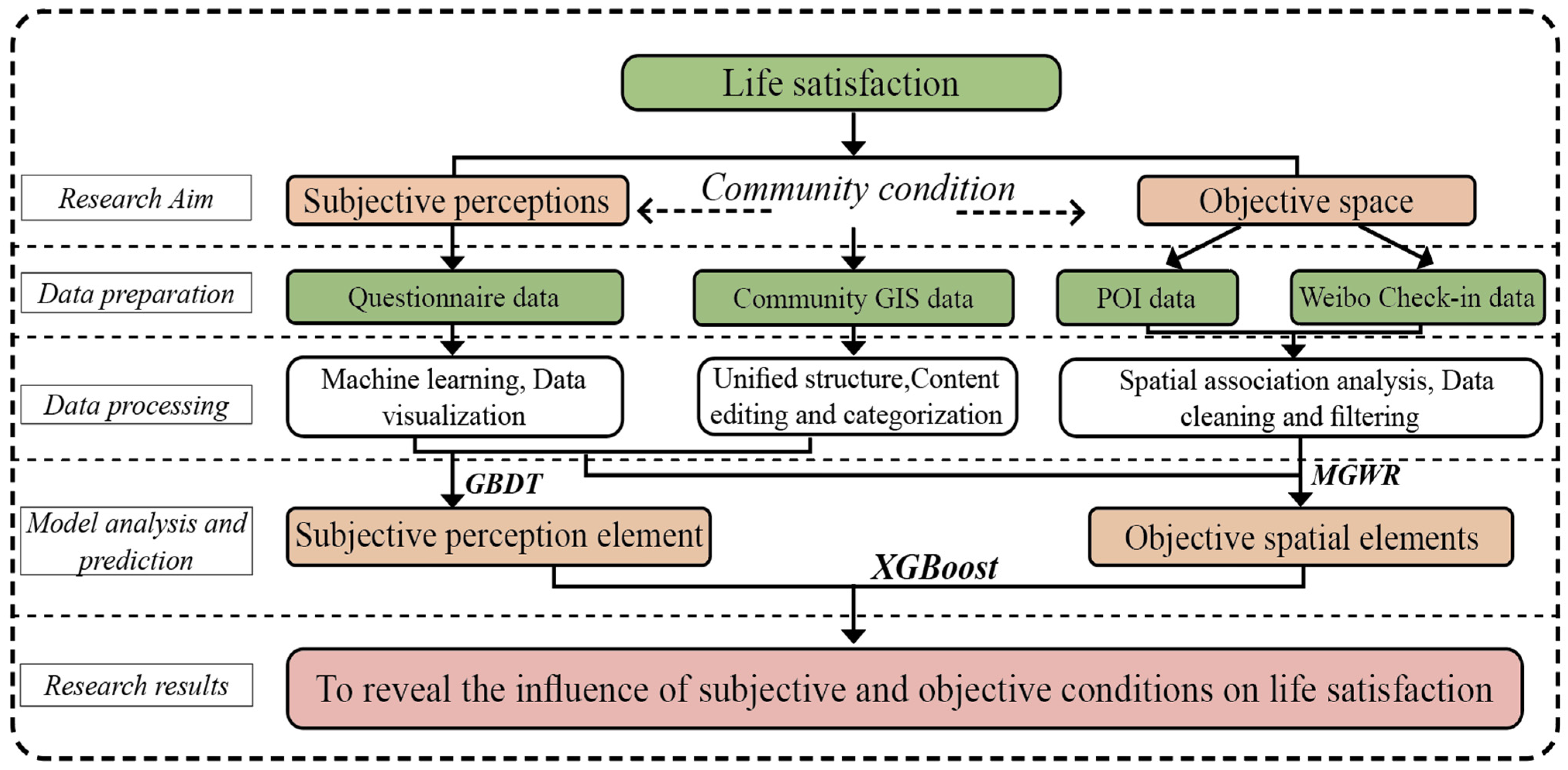
2.4. Research Framework
3. Data and Methods
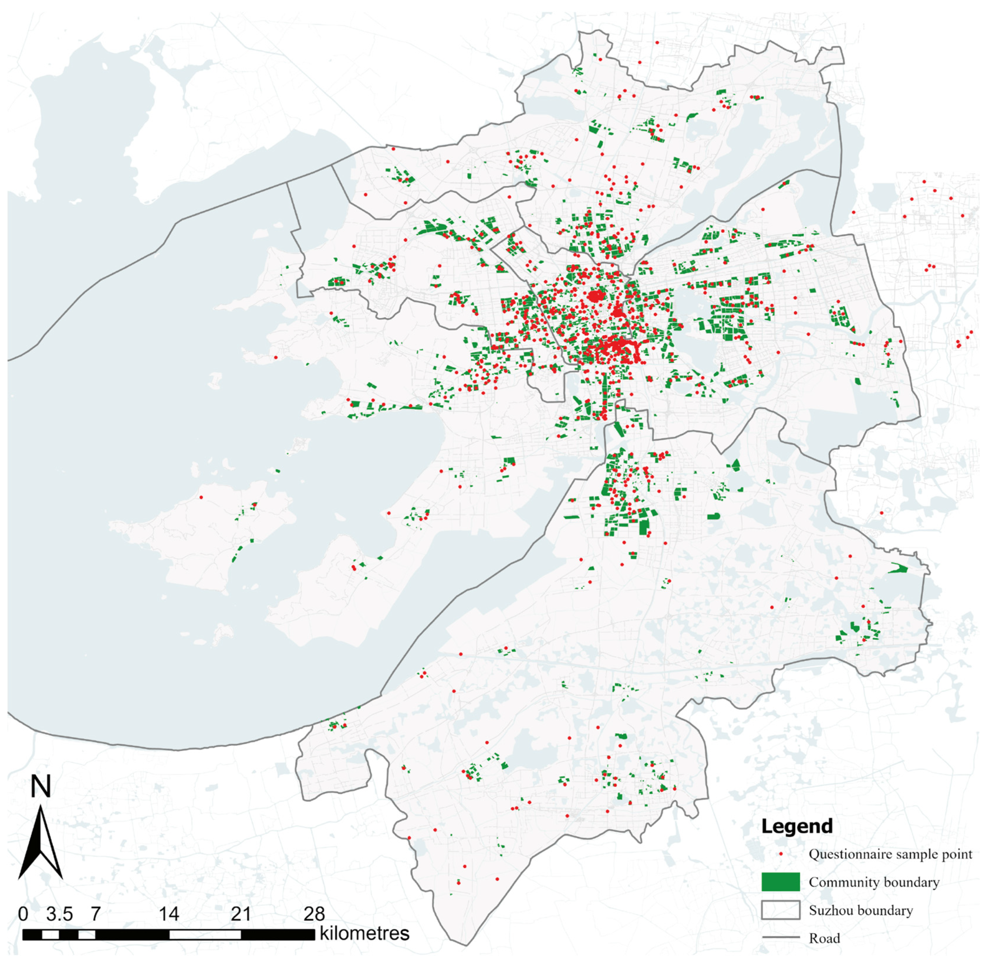
3.1. Research Area
3.2. Methods
3.2.1. MGWR Analysis
- (1)
- OLS regression
- (2)
- Spatial variation test (Moran’s l test)
- (3)
- MGWR analysis
3.2.2. GBDT Analysis
3.2.3. XGBoost Analysis
3.3. Data Collection
4. Results
4.1. MGWR Results Based on Subjective Perception Data
4.1.1. Spatial Correlation Test and OLS Regression Results Based on Subjective Data
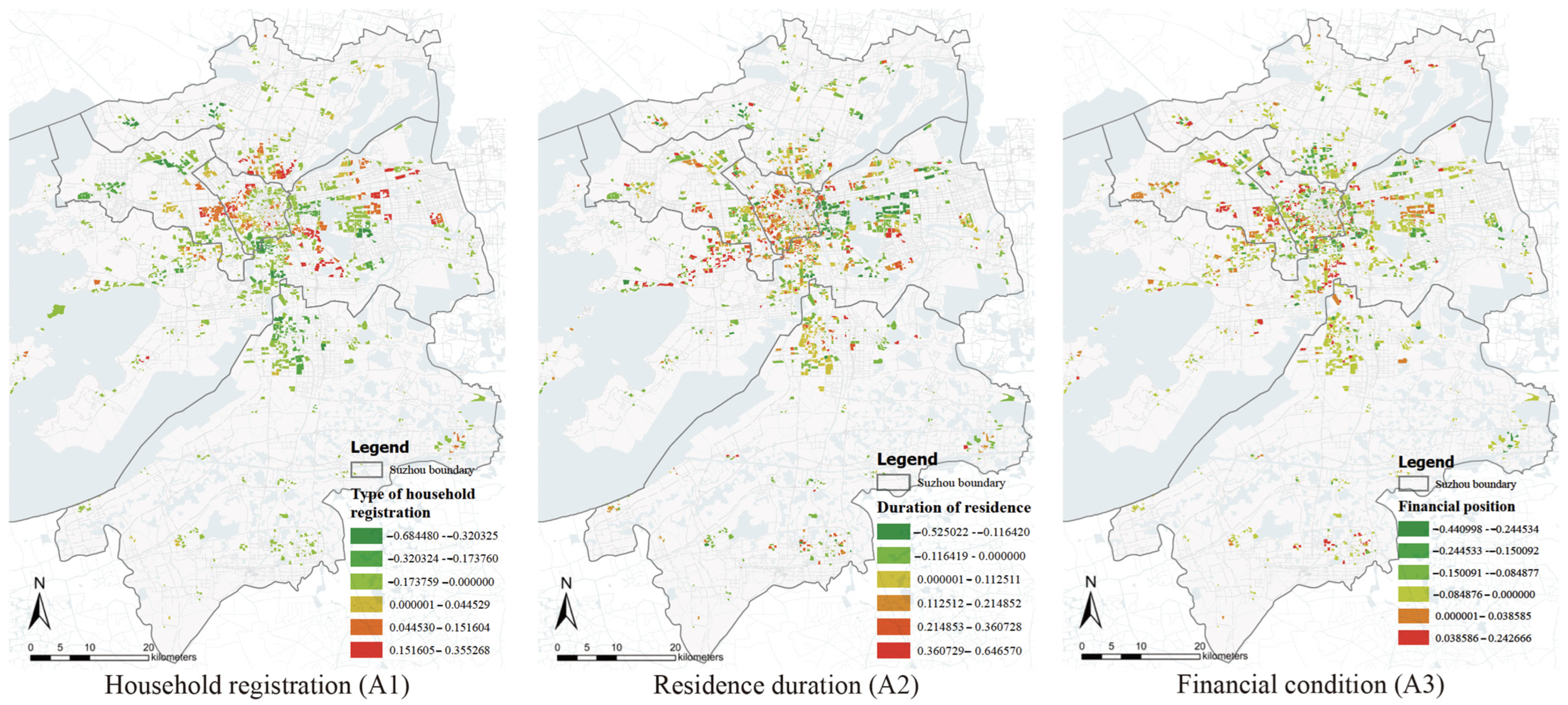
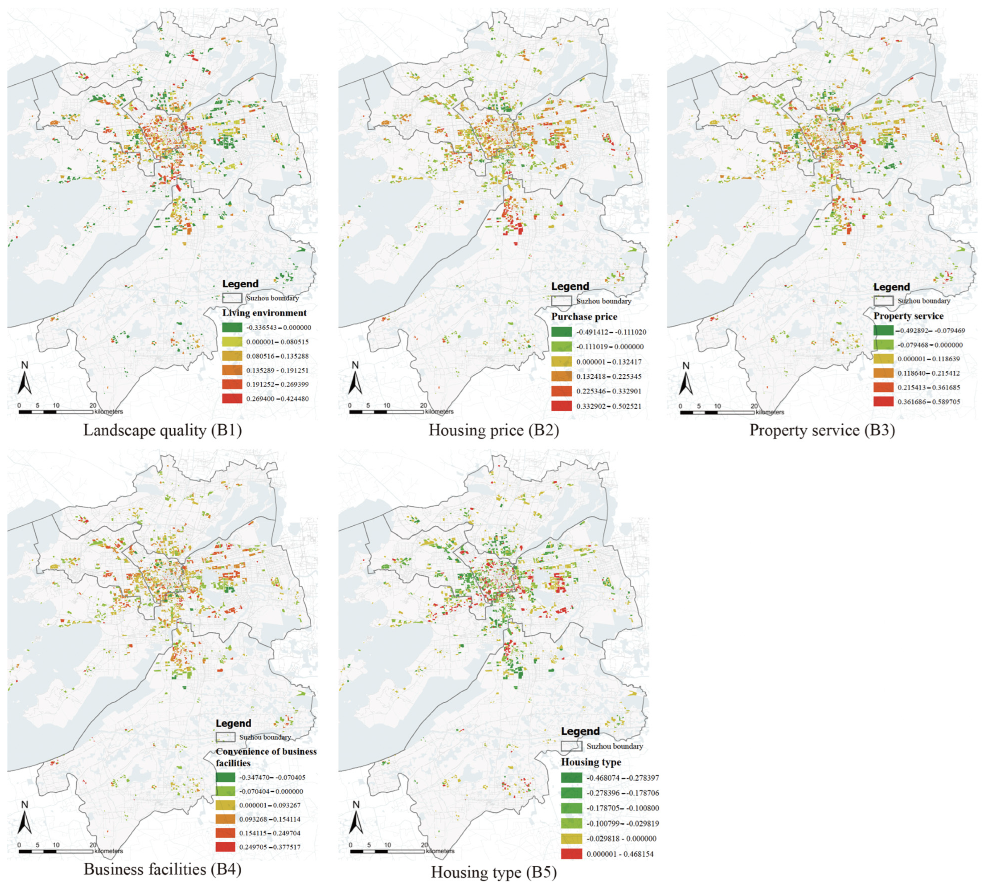
4.1.2. MGWR Analysis Based on Subjective Perception Data
4.2. MGWR Results Based on Objective Geospatial and Social Media Data
4.2.1. Spatial Correlation Test and OLS Regression Results Based on Quantitative Data
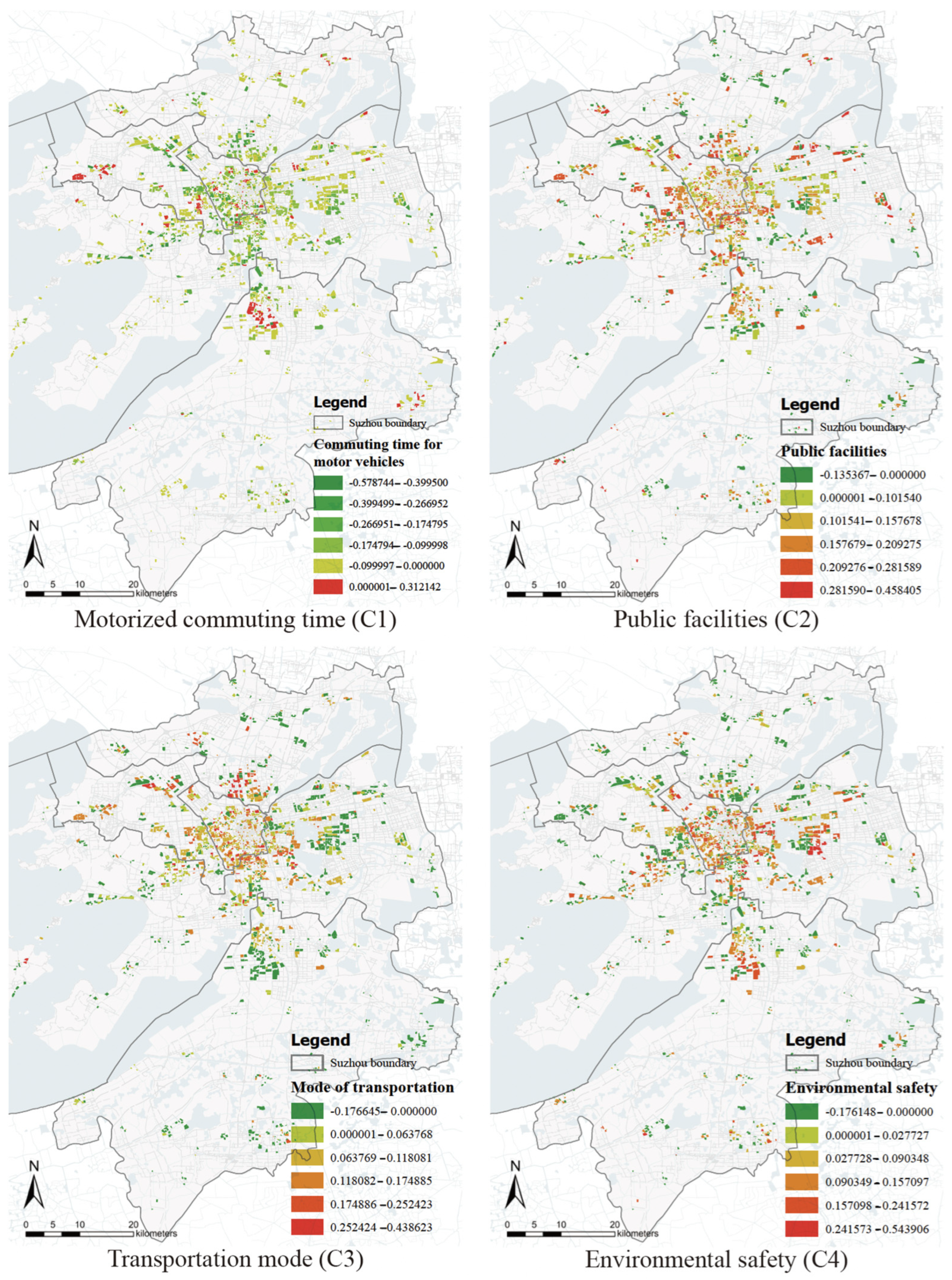
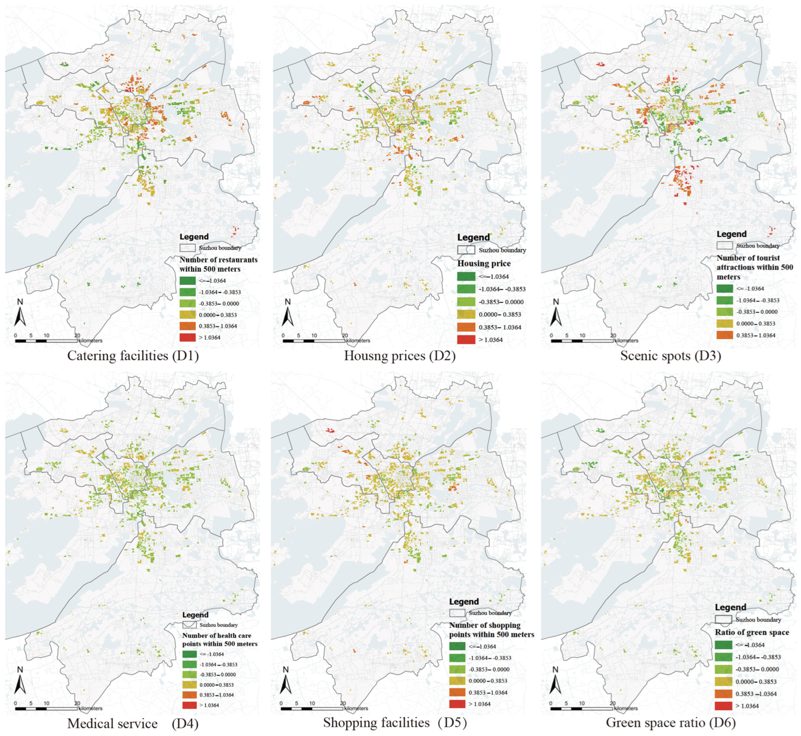
4.2.2. MGWR Results via Objective Geospatial and Social Media Data
4.3. Nonlinear Influential Results via GBDT
4.3.1. Relative Importance of Life Satisfaction Factors
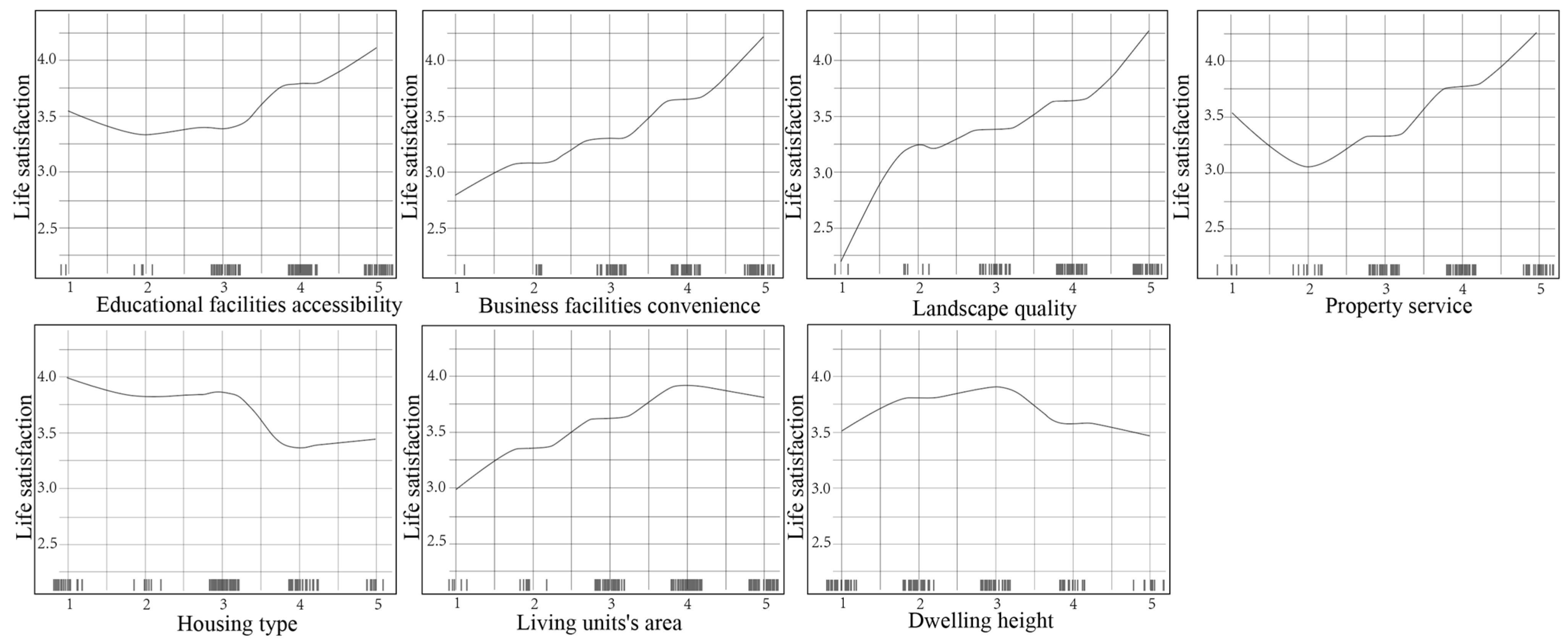
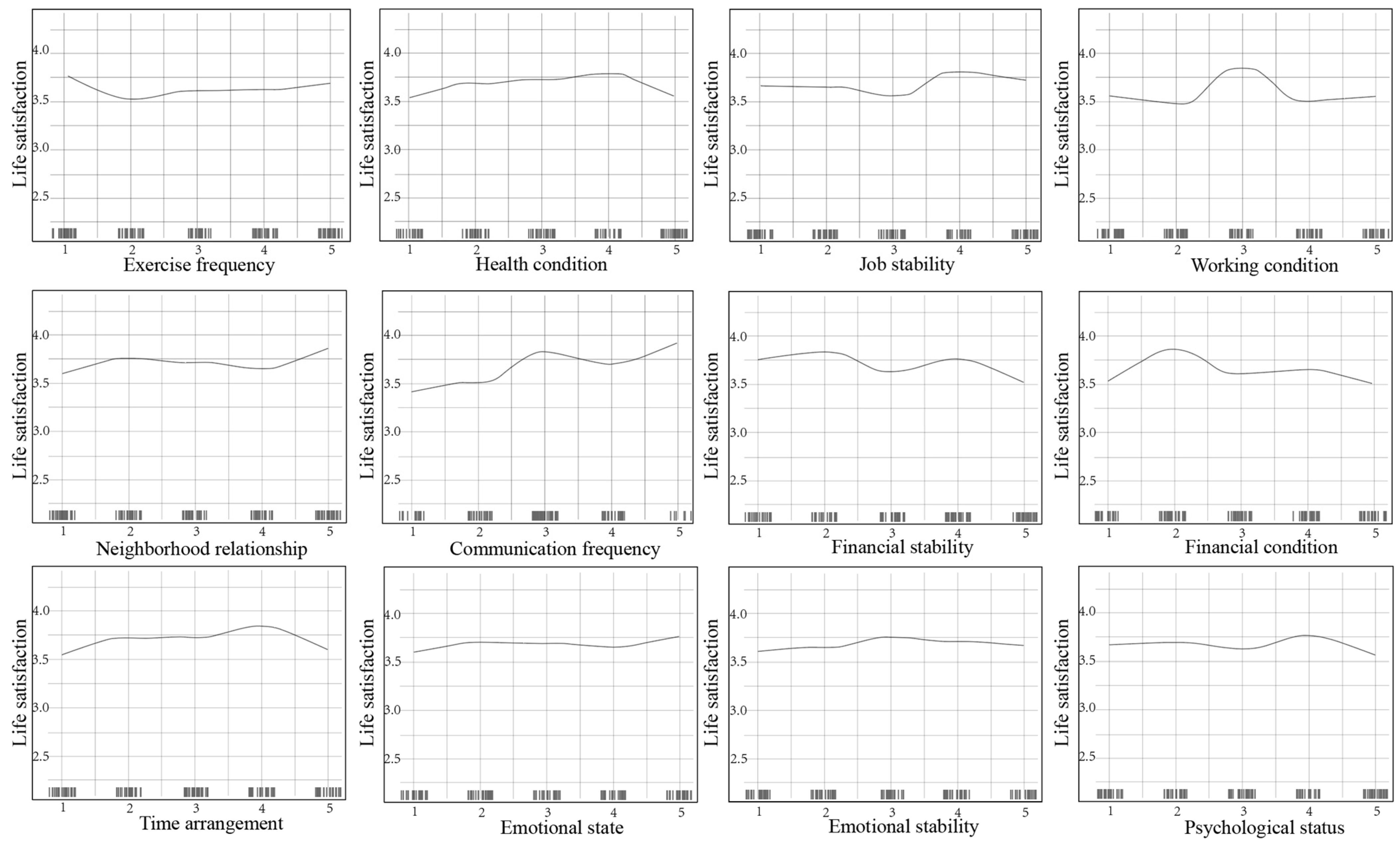
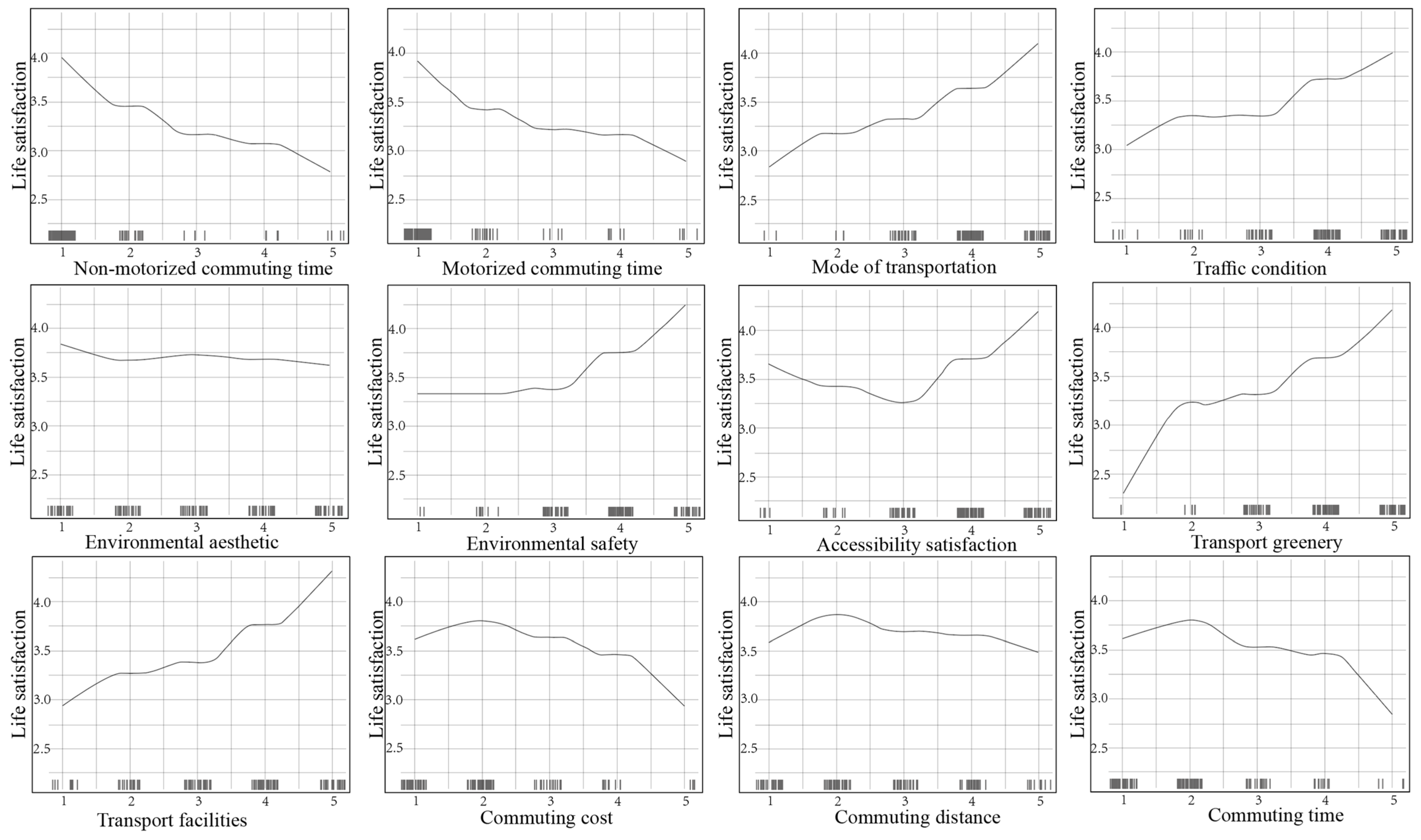
4.3.2. Nonlinear Relationship Between Factors and Life Satisfaction
5. Discussion
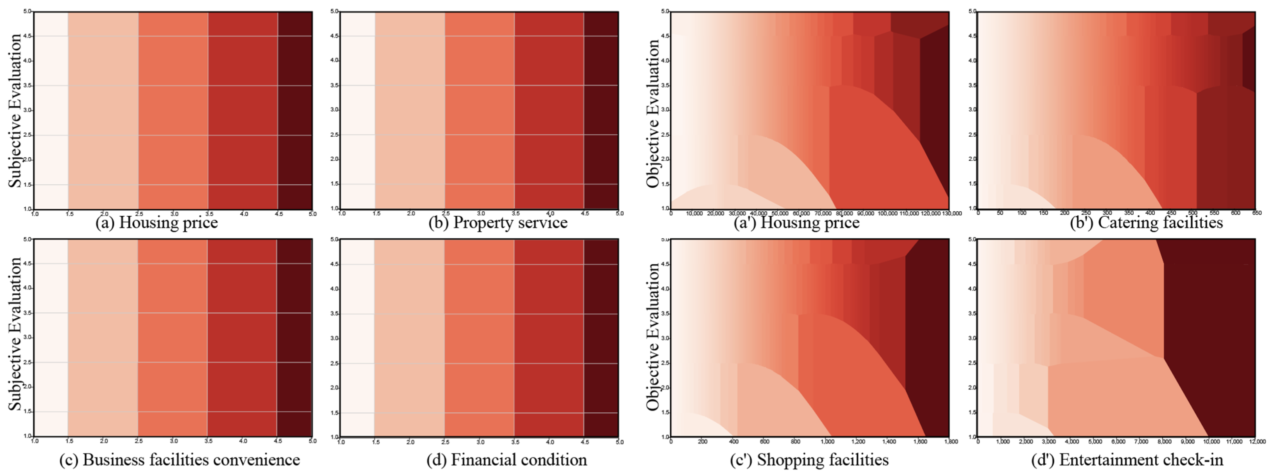
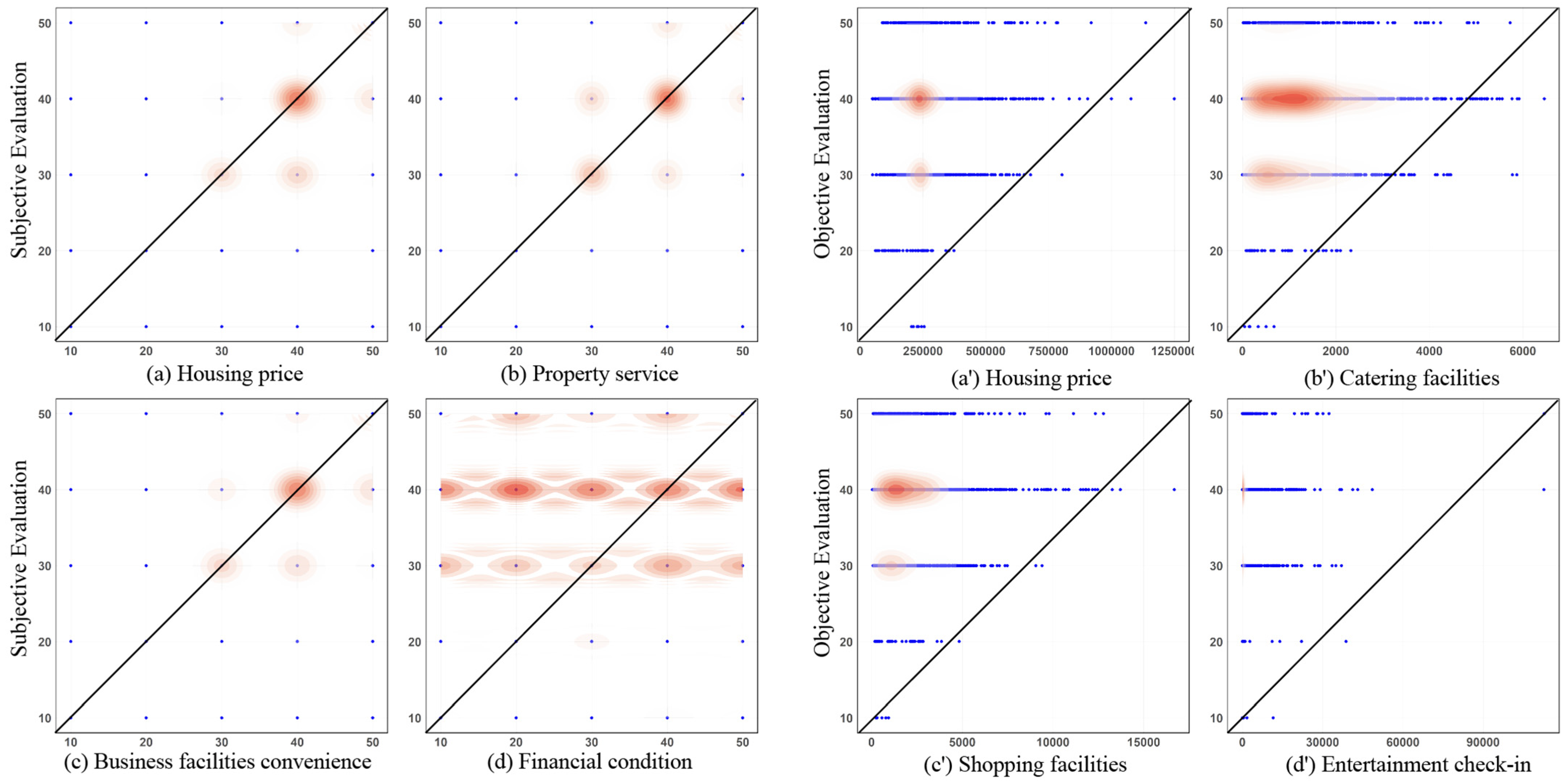
5.1. Subjective Perception and Objective Geospatial Data Result Comparison
5.2. Nonlinear and Prediction Factors Impact on Life Satisfaction
- (1)
- Nonlinear via GBDT
- (2)
- Prediction via XGBoost
5.3. Governance Mechanisms for Improving Life Satisfaction
6. Conclusions
Author Contributions
Funding
Data Availability Statement
Conflicts of Interest
Appendix A

| Items | Questionnaire Variable | Specific Options |
|---|---|---|
| Social Demographics | Age | 1 = 20–25; 2 = 26–30; 3 = 31–35; 4 = 36–40; 5 > 40; |
| Educational background | 1 = Junior high school and below; 2 = High school; 3 = Specialized program; 4 = Bachelor’s degree; 5 = Graduate student or above; | |
| Household registration type | 1 = Local; 2 = Rural local; 3 = Urban migrant; 4 = Rural migrant; 5 = Collective; | |
| Household income | 1 ≤ 5000 RMB; 2 = 10,000–15,000 RMB; 3 = 15,001–25,000 RMB; 4 = 25,001–45,000 RMB; 5 ≥ 45,001 RMB; | |
| Family members | 1 < 2; 2 = 2–3; 3 = 3–4; 4 = 5–6; 5 > 6; | |
| Housing price | 1 = Very cheap; 2 = Cheap; 3 = General; 4 = Exceeding the average value; 5 = Very high; | |
| Gender | 1 = Male; 2= Female; | |
| Residence duration | 1 < 6 months; 2 = 6 months to 1 year; 3 = 1–3 years; 4 = 3–5 years; 5 > 5 years; | |
| Built Environment | Housing type | 1 = Ordinary residence; 2 = Apartment; 3 = Villa; 4 = Bungalow; 5 = Other. |
| Dwelling height | 1 < 3 floors; 2 = 4–6 floors; 3 = 7–11 floors; 4 = 12–18 floors; 5 ≥ 19 floors; | |
| Living units’ area | 1 = 0–45 square meter; 2 = 45–60 square meter; 3 = 61–90 square meter; 4 = 91–120 square meter; 5 > 120 square meter; | |
| Property services | 1 = Strongly dissatisfied <——> 5 = Strongly satisfied | |
| Landscape quality | 1 = Strongly dissatisfied <——> 5 = Strongly satisfied | |
| Educational facilities accessibility | 1 = Strongly dissatisfied <——> 5 = Strongly satisfied | |
| Business facilities convenience | 1 = Strongly dissatisfied <——> 5 = Strongly satisfied | |
| Social Interaction | Neighborhood relationship | 1 = Strongly dissatisfied <——> 5 = Strongly satisfied |
| Work status | 1 = Strongly dissatisfied <——> 5 = Strongly satisfied | |
| Job stability | 1 = Strongly dissatisfied <——> 5 = Strongly satisfied | |
| Health condition | 1 = Strongly dissatisfied <——> 5 = Strongly satisfied | |
| Communication frequency | 1 < 2; 2 = 2–4; 3 = 5–8; 4 = 9–12; 5 ≥ 13; | |
| Exercise frequency | 1 < 2; 2 = 2–4; 3 = 5–8; 4 = 9–12; 5 ≥ 13; | |
| Psychological status | 1 = Strongly dissatisfied <——> 5 = Strongly satisfied | |
| Emotional stability | 1 = Strongly dissatisfied <——> 5 = Strongly satisfied | |
| Emotional state | 1 = Strongly dissatisfied <——> 5 = Strongly satisfied | |
| Time arrangement | 1 = Strongly dissatisfied <——> 5 = Strongly satisfied | |
| Financial condition | 1 = Strongly dissatisfied <——> 5 = Strongly satisfied | |
| Financial stability | 1 = Strongly dissatisfied <——> 5 = Strongly satisfied | |
| Commuting Environment | Commuting time | 1 ≤ 20 min; 2 = 21–40 min; 3 = 41–60 min; 4 = 61–80 min; 5 ≥ 80 min; |
| Commuting distance | 1 ≤ 3 km; 2 = 3–6 km; 3 = 6–9 km; 4 = 9–16 km; 5 > 16 km; | |
| Commuting cost | 1 = Strongly dissatisfied <——> 5 = Strongly satisfied | |
| Transport facilities | 1 = Strongly dissatisfied <——> 5 = Strongly satisfied | |
| Transport greenery | 1 = Strongly dissatisfied <——> 5 = Strongly satisfied | |
| Accessibility services | 1 = Strongly dissatisfied <——> 5 = Strongly satisfied | |
| Environmental cleanliness | 1 = Strongly dissatisfied <——> 5 = Strongly satisfied | |
| Environmental safety | 1 = Strongly dissatisfied <——> 5 = Strongly satisfied | |
| Environmental aesthetic | 1 = Strongly dissatisfied <——> 5 = Strongly satisfied | |
| Traffic condition | 1 = Strongly dissatisfied <——> 5 = Strongly satisfied | |
| Mode of transportation | 1 = Strongly dissatisfied <——> 5 = Strongly satisfied | |
| Motorized commuting time | 1 = 0; 2 = 1; 3 = 2; 4 = 3–4; 5 > 4; | |
| Non-motorized commuting time | 1 = 0; 2 = 1; 3 = 2; 4 = 3–4; 5 > 4; |
References
- Kim, G.; Newman, G.; Jiang, B. Urban Regeneration: Community Engagement Process for Vacant Land in Declining Cities. Cities 2020, 102, 102730. [Google Scholar] [CrossRef] [PubMed]
- Mayer, B.; Joshweseoma, L.; Sehongva, G. Environmental Risk Perceptions and Community Health: Arsenic, Air Pollution, and Threats to Traditional Values of the Hopi Tribe. J. Community Health 2019, 44, 896–902. [Google Scholar] [CrossRef] [PubMed]
- Liu, G.; Wei, L.; Gu, J.; Zhou, T.; Liu, Y. Benefit Distribution in Urban Renewal from the Perspectives of Efficiency and Fairness: A Game Theoretical Model and the Government’s Role in China. Cities 2020, 96, 102422. [Google Scholar] [CrossRef]
- Guterres, A. The Sustainable Development Goals Report 2023: Special Edition; Department of Economic and Social Affairs: New York, NY, USA, 2023. [Google Scholar]
- Li, X.; Zhou, Y.; Hejazi, M.; Wise, M.; Vernon, C.; Iyer, G.; Chen, W. Global Urban Growth between 1870 and 2100 from Integrated High Resolution Mapped Data and Urban Dynamic Modeling. Commun. Earth Environ. 2021, 2, 201. [Google Scholar] [CrossRef]
- State Council of the PRC Notice of the General Office of the Ministry of Housing and Urban Rural Development on Carrying out the First Batch of Urban Renewal Pilot Work. Available online: https://www.gov.cn/zhengce/zhengceku/2021-11/06/content_5649443.htm (accessed on 10 September 2024).
- Chen, J.; Pellegrini, P.; Wang, H. Comparative Residents’ Satisfaction Evaluation for Socially Sustainable Regeneration—The Case of Two High-Density Communities in Suzhou. Land 2022, 11, 1483. [Google Scholar] [CrossRef]
- Korkmaz, C.; Balaban, O. Sustainability of Urban Regeneration in Turkey: Assessing the Performance of the North Ankara Urban Regeneration Project. Habitat Int. 2020, 95, 102081. [Google Scholar] [CrossRef]
- Bianchi, C.; Bereciartua, P.; Vignieri, V.; Cohen, A. Enhancing Urban Brownfield Regeneration to Pursue Sustainable Community Outcomes through Dynamic Performance Governance. Int. J. Public Adm. 2021, 44, 100–114. [Google Scholar] [CrossRef]
- Shi, J.; Huang, J.; Guo, M.; Tian, L.; Wang, J.; Wong, T.W.; Webster, C.; Leung, G.M.; Ni, M.Y. Contributions of Residential Traffic Noise to Depression and Mental Wellbeing in Hong Kong: A Prospective Cohort Study. Environ. Pollut. 2023, 338, 122641. [Google Scholar] [CrossRef]
- Jiang, C.; Xiao, Y.; Cao, H. Co-Creating for Locality and Sustainability: Design-Driven Community Regeneration Strategy in Shanghai’s Old Residential Context. Sustainability 2020, 12, 2997. [Google Scholar] [CrossRef]
- Zhou, X.; Zhang, X.; Dai, Z.; Hermaputi, R.L.; Hua, C.; Li, Y. Spatial Layout and Coupling of Urban Cultural Relics: Analyzing Historical Sites and Commercial Facilities in District Iii of Shaoxing. Sustainability 2021, 13, 6877. [Google Scholar] [CrossRef]
- Turel, H.S.; Yigit, E.M.; Altug, I. Evaluation of Elderly People’s Requirements in Public Open Spaces: A Case Study in Bornova District (Izmir, Turkey). Build. Environ. 2007, 42, 2035–2045. [Google Scholar] [CrossRef]
- Williams, P.; Pocock, B. Building “community” for Different Stages of Life: Physical and Social Infrastructure in Master Planned Communities. Community Work Fam. 2010, 13, 71–87. [Google Scholar] [CrossRef]
- Yang, L.; Ho, J.Y.S.; Wong, F.K.Y.; Chang, K.K.P.; Chan, K.L.; Wong, M.S.; Ho, H.C.; Yuen, J.W.M.; Huang, J.; Siu, J.Y.M. Neighbourhood Green Space, Perceived Stress and Sleep Quality in an Urban Population. Urban For. Urban Green. 2020, 54, 126763. [Google Scholar] [CrossRef]
- Cheung, T.; Graham, L.T.; Schiavon, S. Impacts of Life Satisfaction, Job Satisfaction and the Big Five Personality Traits on Satisfaction with the Indoor Environment. Build. Environ. 2022, 212, 108783. [Google Scholar] [CrossRef]
- Couch, C.; Sykes, O.; Börstinghaus, W. Thirty Years of Urban Regeneration in Britain, Germany and France: The Importance of Context and Path Dependency. Prog. Plan. 2011, 75, 1–52. [Google Scholar] [CrossRef]
- Cao, J. The Association between Light Rail Transit and Satisfactions with Travel and Life: Evidence from Twin Cities. Transportation 2013, 40, 921–933. [Google Scholar] [CrossRef]
- Lee, K.S.; You, S.Y.; Eom, J.K.; Song, J.; Min, J.H. Urban Spatiotemporal Analysis Using Mobile Phone Data: Case Study of Medium- and Large-Sized Korean Cities. Habitat Int. 2018, 73, 6–15. [Google Scholar] [CrossRef]
- Li, X.; Li, Y.; Jia, T.; Zhou, L.; Hijazi, I.H. The Six Dimensions of Built Environment on Urban Vitality: Fusion Evidence from Multi-Source Data. Cities 2022, 121, 103482. [Google Scholar] [CrossRef]
- Song, H.; Chen, J.; Li, P. Decoding the cultural heritage tourism landscape and visitor crowding behavior from the multidimensional embodied perspective: Insights from Chinese classical gardens. Tour. Manag. 2025, 110, 105180. [Google Scholar] [CrossRef]
- Zeng, C.; Song, Y.; He, Q.; Shen, F. Spatially Explicit Assessment on Urban Vitality: Case Studies in Chicago and Wuhan. Sustain. Cities Soc. 2018, 40, 296–306. [Google Scholar] [CrossRef]
- Chen, J.; Pellegrini, P.; Xu, Y.; Ma, G.; Wang, H.; An, Y.; Shi, Y.; Feng, X. Evaluating Residents’ Satisfaction before and after Regeneration. The Case of a High-Density Resettlement Neighbourhood in Suzhou, China. Cogent Soc. Sci. 2022, 8, 2144137. [Google Scholar] [CrossRef]
- Huang, J.; Cui, Y.; Li, L.; Guo, M.; Ho, H.C.; Lu, Y.; Webster, C. Re-Examining Jane Jacobs’ Doctrine Using New Urban Data in Hong Kong. Environ. Plan. B Urban Anal. City Sci. 2023, 50, 76–93. [Google Scholar] [CrossRef]
- Xiao, L.; Lo, S.; Liu, J.; Zhou, J.; Li, Q. Nonlinear and Synergistic Effects of TOD on Urban Vibrancy: Applying Local Explanations for Gradient Boosting Decision Tree. Sustain. Cities Soc. 2021, 72, 103063. [Google Scholar] [CrossRef]
- Li, W. Unveiling Fine-Scale Urban Third Places for Remote Work Using Mobile Phone Big Data. Sustain. Cities Soc. 2024, 103, 105258. [Google Scholar] [CrossRef]
- Cao, X. (Jason) How Does Neighborhood Design Affect Life Satisfaction? Evidence from Twin Cities. Travel Behav. Soc. 2016, 5, 68–76. [Google Scholar] [CrossRef]
- Zhou, K.; Tan, J.; Watanabe, K. How Does Perceived Residential Environment Quality Influence Life Satisfaction? Evidence from Urban China. J. Community Psychol. 2021, 49, 2454–2471. [Google Scholar] [CrossRef]
- Gao, M.; Ahern, J.; Koshland, C.P. Perceived Built Environment and Health-Related Quality of Life in Four Types of Neighborhoods in Xi’an, China. Health Place 2016, 39, 110–115. [Google Scholar] [CrossRef]
- Zhang, Z.; Zhang, J. Perceived Residential Environment of Neighborhood and Subjective Well-Being among the Elderly in China: A Mediating Role of Sense of Community. J. Environ. Psychol. 2017, 51, 82–94. [Google Scholar] [CrossRef]
- Sadeghi, A.R.; Ebadi, M.; Shams, F.; Jangjoo, S. Human-Built Environment Interactions: The Relationship between Subjective Well-Being and Perceived Neighborhood Environment Characteristics. Sci. Rep. 2022, 12, 21844. [Google Scholar] [CrossRef]
- Sassen, S. Cities in a World Economy; Sage Publications: Thousand Oaks, CA, USA, 2018; ISBN 1-5063-6262-1. [Google Scholar]
- Harvey, D. Social Justice and the City; University of Georgia Press: Athens, GA, USA, 2010; Volume 1, ISBN 0820336041. [Google Scholar]
- Shi, X.; Li, X.; Chen, X.; Zhang, L. Objective Air Quality Index versus Subjective Perception: Which Has a Greater Impact on Life Satisfaction? Environ. Dev. Sustain. 2022, 24, 6860–6877. [Google Scholar] [CrossRef]
- Xiao, Y.; Miao, S.; Zhang, Y.; Chen, H.; Wu, W. Exploring the Health Effects of Neighborhood Greenness on Lilong Residents in Shanghai. Urban For. Urban Green. 2021, 66, 127383. [Google Scholar] [CrossRef]
- Wu, W.; Yun, Y.; Hu, B.; Sun, Y.; Xiao, Y. Greenness, Perceived Pollution Hazards and Subjective Wellbeing: Evidence from China. Urban For. Urban Green. 2020, 56, 126796. [Google Scholar] [CrossRef]
- Liu, Y.; Zhang, F.; Wu, F.; Liu, Y.; Li, Z. The Subjective Wellbeing of Migrants in Guangzhou, China: The Impacts of the Social and Physical Environment. Cities 2017, 60, 333–342. [Google Scholar] [CrossRef]
- Lynch, K. The Image of the City (1960); Gebr. Mann Verlag: Berlin, Germany, 2023; pp. 481–488. [Google Scholar]
- Jacobs, J.M. Re-Making Public Space through and in Asia. In Public Space in Urban Asia; World Scientific: Singapore, 2013; pp. 186–189. ISBN 978-981-4578-32-5. [Google Scholar]
- Ambrey, C.; Fleming, C. Public Greenspace and Life Satisfaction in Urban Australia. Urban Stud. 2014, 51, 1290–1321. [Google Scholar]
- Xie, B.; An, Z.; Zheng, Y.; Li, Z. Healthy Aging with Parks: Association between Park Accessibility and the Health Status of Older Adults in Urban China. Sustain. Cities Soc. 2018, 43, 476–486. [Google Scholar] [CrossRef]
- Mouratidis, K. Commute Satisfaction, Neighborhood Satisfaction, and Housing Satisfaction as Predictors of Subjective Well-Being and Indicators of Urban Livability. Travel Behav. Soc. 2020, 21, 265–278. [Google Scholar] [CrossRef]
- Kubiszewski, I.; Zakariyya, N.; Costanza, R. Objective and Subjective Indicators of Life Satisfaction in Australia: How Well Do People Perceive What Supports a Good Life? Ecolog. Econ. 2018, 154, 361–372. [Google Scholar]
- Willroth, E.C.; John, O.P.; Biesanz, J.C.; Mauss, I.B. Understanding Short-Term Variability in Life Satisfaction: The Individual Differences in Evaluating Life Satisfaction (IDELS) Model. J. Pers. Soc. Psychol. 2020, 119, 229. [Google Scholar] [CrossRef]
- Zhang, S.X.; Wang, Y.; Rauch, A.; Wei, F. Unprecedented Disruption of Lives and Work: Health, Distress and Life Satisfaction of Working Adults in China One Month into the COVID-19 Outbreak. Psychiatry Res. 2020, 288, 112958. [Google Scholar] [CrossRef] [PubMed]
- Suls, J.; Wills, T.A. Social Comparison: Contemporary Theory and Research; Taylor & Francis: Oxford, UK, 2024; ISBN 1-040-02559-5. [Google Scholar]
- Fan, L.; Cao, J.; Hu, M.; Yin, C. Exploring the Importance of Neighborhood Characteristics to and Their Nonlinear Effects on Life Satisfaction of Displaced Senior Farmers. Cities 2022, 124, 103605. [Google Scholar] [CrossRef]
- Ding, J.; Salinas-Jiménez, J.; Salinas-Jiménez, M.d.M. The Impact of Income Inequality on Subjective Well-Being: The Case of China. J. Happiness Stud. 2021, 22, 845–866. [Google Scholar] [CrossRef]
- Hansen, T.; Blekesaune, M. The Age and Well-Being “Paradox”: A Longitudinal and Multidimensional Reconsideration. Eur. J. Ageing 2022, 19, 1277–1286. [Google Scholar] [CrossRef] [PubMed]
- Kim, E.S.; Delaney, S.W.; Tay, L.; Chen, Y.; Diener, E.; Vanderweele, T.J. Life Satisfaction and Subsequent Physical, Behavioral, and Psychosocial Health in Older Adults. Milbank Q. 2021, 99, 209–239. [Google Scholar] [CrossRef] [PubMed]
- Levin, K.A.; Torsheim, T.; Vollebergh, W.; Richter, M.; Davies, C.A.; Schnohr, C.W.; Due, P.; Currie, C. National Income and Income Inequality, Family Affluence and Life Satisfaction among 13 Year Old Boys and Girls: A Multilevel Study in 35 Countries. Soc. Indic. Res. 2011, 104, 179–194. [Google Scholar] [CrossRef]
- Wan, T.; Lu, W.; Na, X.; Rong, W. Non-Linear Impact of Economic Performance on Social Equity in Rail Transit Station Areas. Sustainability 2024, 16, 6518. [Google Scholar] [CrossRef]
- Gao, L.; Chong, H.-Y.; Zhang, W.; Li, Z. Nonlinear Effects of Public Transport Accessibility on Urban Development: A Case Study of Mountainous City. Cities 2023, 138, 104340. [Google Scholar] [CrossRef]
- Ingenfeld, J.; Wolbring, T.; Bless, H. Commuting and Life Satisfaction Revisited: Evidence on a Non-Linear Relationship. J. Happiness Stud. 2019, 20, 2677–2709. [Google Scholar] [CrossRef]
- Atienza-González, F.L.; Martínez, N.; Silva, C. Life Satisfaction and Self-Rated Health in Adolescents: The Relationships between Them and the Role of Gender and Age. Span. J. Psychol. 2020, 23, e4. [Google Scholar] [CrossRef]
- Ren, D.; Stavrova, O.; Loh, W.W. Nonlinear Effect of Social Interaction Quantity on Psychological Well-Being: Diminishing Returns or Inverted U? J. Pers. Soc. Psychol. 2022, 122, 1056. [Google Scholar] [CrossRef]
- Yin, C.; Shao, C. Revisiting Commuting, Built Environment and Happiness: New Evidence on a Nonlinear Relationship. Transp. Res. Part D Transp. Environ. 2021, 100, 103043. [Google Scholar] [CrossRef]
- Dong, Y.; Sun, Y.; Waygood, E.O.D.; Wang, B.; Huang, P.; Naseri, H. Insight into the Nonlinear Effect of COVID-19 on Well-Being in China: Commuting, a Vital Ingredient. J. Transp. Health 2022, 27, 101526. [Google Scholar] [CrossRef] [PubMed]
- Wu, C.; Yang, S.; Ma, Y.; Liu, P.; Ye, X. Urban Green Space Assessment: Spatial Clustering Method Based on Multisource Data to Facilitate Zoning Planning. J. Urban Plann. Dev. 2024, 150, 4024032. [Google Scholar] [CrossRef]
- De Vos, J.; Schwanen, T.; Van Acker, V.; Witlox, F. Travel and Subjective Well-Being: A Focus on Findings, Methods and Future Research Needs. Transp. Rev. 2013, 33, 421–442. [Google Scholar] [CrossRef]
- Kroesen, M. Assessing Mediators in the Relationship between Commute Time and Subjective Well-Being: Structural Equation Analysis. Transp. Res. Rec. 2014, 2452, 114–123. [Google Scholar] [CrossRef]
- Dong, L.; Jiang, H.; Li, W.; Qiu, B.; Wang, H.; Qiu, W. Assessing Impacts of Objective Features and Subjective Perceptions of Street Environment on Running Amount: A Case Study of Boston. Landsc. Urban Plann. 2023, 235, 104756. [Google Scholar] [CrossRef]
- Qiu, W.; Zhang, Z.; Liu, X.; Li, W.; Li, X.; Xu, X.; Huang, X. Subjective or Objective Measures of Street Environment, Which Are More Effective in Explaining Housing Prices? Landsc. Urban Plann. 2022, 221, 104358. [Google Scholar] [CrossRef]
- Qiu, W.; Li, W.; Liu, X.; Zhang, Z.; Li, X.; Huang, X. Subjective and Objective Measures of Streetscape Perceptions: Relationships with Property Value in Shanghai. Cities 2023, 132, 104037. [Google Scholar] [CrossRef]
- Li, L.; Wu, X.; Kong, M.; Liu, J.; Zhang, J. Quantitatively Interpreting Residents Happiness Prediction by Considering Factor–Factor Interactions. IEEE Trans. Comput. Soc. Syst. 2023, 11, 1402–1414. [Google Scholar] [CrossRef]
- He, X.; Zhou, Y.; Yuan, X.; Zhu, M. The Coordination Relationship between Urban Development and Urban Life Satisfaction in Chinese Cities—An Empirical Analysis Based on Multi-Source Data. Cities 2024, 150, 105016. [Google Scholar] [CrossRef]
- Chen, J.; Li, P.; Wang, H. Assessment of Influential Factors on Commute and Life Satisfaction in a Historic Campus-Adjacent Environment: Evidence from a Comparison Study of Twin Cities. J. Urban Plann. Dev. 2025, 151, 4024065. [Google Scholar] [CrossRef]
- Chen, J.; Tian, W.; Xu, K.; Pellegrini, P. Testing Small-Scale Vitality Measurement Based on 5D Model Assessment with Multi-Source Data: A Resettlement Community Case in Suzhou. ISPRS Int. J. Geo-Inf. 2022, 11, 626. [Google Scholar] [CrossRef]
- Zhang, L.; Li, X.; Guo, Y. Research on the Influencing Factors of Spatial Vitality of Night Parks Based on AHP–Entropy Weights. Sustainability 2024, 16, 5165. [Google Scholar] [CrossRef]
- Zhao, M.; Liu, N.; Chen, J.; Wang, D.; Li, P.; Yang, D.; Zhou, P. Navigating Post-COVID-19 Social–Spatial Inequity: Unravelling the Nexus between Community Conditions, Social Perception, and Spatial Differentiation. Land 2024, 13, 563. [Google Scholar] [CrossRef]
- Zhang, X.; Chen, J.; Wang, H.; Yang, D. From Policy Synergy to Equitable Greenspace: Unveiling the Multifaceted Effects of Regional Cooperation upon Urban Greenspace Exposure Inequality in China’s Megacity-Regions. Appl. Geogr. 2025, 174, 103472. [Google Scholar]
- Chen, J.; Gan, W.; Liu, N.; Li, P.; Wang, H.; Zhao, X.; Yang, D. Community Quality Evaluation for Socially Sustainable Regeneration: A Study Using Multi-Sourced Geospatial Data and AI-Based Image Semantic Segmentation. ISPRS Int. J. Geo-Inf. 2024, 13, 167. [Google Scholar] [CrossRef]
- Ma, G.; Pellegrini, P.; Wu, H.; Han, H.; Wang, D.; Chen, J. Impact of Land-Use Mixing on the Vitality of Urban Parks: Evidence from Big Data Analysis in Suzhou, Yangtze River Delta Region, China. J. Urban Plann. Dev. 2023, 149, 4023045. [Google Scholar] [CrossRef]
- Chen, J.; Zhao, X.; Wang, H.; Yan, J.; Yang, D.; Xie, K. Portraying Heritage Corridor Dynamics and Cultivating Conservation Strategies Based on Environment Spatial Model: An Integration of Multi-Source Data and Image Semantic Segmentation. Herit. Sci. 2024, 12, 419. [Google Scholar]
- Xu, X.; Qiu, W.; Li, W.; Liu, X.; Zhang, Z.; Li, X.; Luo, D. Associations between Street-View Perceptions and Housing Prices: Subjective vs. Objective Measures Using Computer Vision and Machine Learning Techniques. Remote Sens. 2022, 14, 891. [Google Scholar] [CrossRef]
- Kubiszewski, I.; Mulder, K.; Jarvis, D.; Costanza, R. Toward Better Measurement of Sustainable Development and Wellbeing: A Small Number of SDG Indicators Reliably Predict Life Satisfaction. Sustain. Dev. 2022, 30, 139–148. [Google Scholar] [CrossRef]
- Wang, R.; Zhang, G.; Zhang, Y.; Lan, Y. Exploring the Spatially Heterogeneous Effects of Street-Level Perceived Qualities on Listed Real Estate Prices Using Geographically Weighted Regression (GWR) Modeling. Buildings 2024, 14, 1982. [Google Scholar] [CrossRef]
- Nkeki, F.N.; Asikhia, M.O. Geographically Weighted Logistic Regression Approach to Explore the Spatial Variability in Travel Behaviour and Built Environment Interactions: Accounting Simultaneously for Demographic and Socioeconomic Characteristics. Appl. Geogr. 2019, 108, 47–63. [Google Scholar] [CrossRef]
- Zhu, P.; Li, J.; Wang, K.; Huang, J. Exploring Spatial Heterogeneity in the Impact of Built Environment on Taxi Ridership Using Multiscale Geographically Weighted Regression. Transportation 2024, 51, 1963–1997. [Google Scholar] [CrossRef]
- Wu, W.; Tan, W.; Chen, W.Y.; Wang, R. Disentangling the Non-Linear Impacts of Natural Attributes of Urban Built Environment on Life Satisfaction. Cities 2024, 155, 105496. [Google Scholar] [CrossRef]
- Zhou, S.; Liu, Z.; Wang, M.; Gan, W.; Zhao, Z.; Wu, Z. Impacts of Building Configurations on Urban Stormwater Management at a Block Scale Using XGBoost. Sustain. Cities Soc. 2022, 87, 104235. [Google Scholar] [CrossRef]
- Sanders, W.; Li, D.; Li, W.; Fang, Z.N. Data-Driven Flood Alert System (FAS) Using Extreme Gradient Boosting (XGBoost) to Forecast Flood Stages. Water 2022, 14, 747. [Google Scholar] [CrossRef]
- Wang, L.; Shen, J.; Chung, C.K.L. City Profile: Suzhou-a Chinese City under Transformation. Cities 2015, 44, 60–72. [Google Scholar]
- Liang, X.; Jin, X.; Ren, J.; Gu, Z.; Zhou, Y. A Research Framework of Land Use Transition in Suzhou City Coupled with Land Use Structure and Landscape Multifunctionality. Sci. Total Environ. 2020, 737, 139932. [Google Scholar]
- Ye, Y.; Huang, R.; Zhang, L. Human-Oriented Urban Design with Support of Multi-Source Data and Deep Learning: A Case Study on Urban Greenway Planning of Suzhou Creek, Shanghai. Landsc. Archit. 2021, 28, 39–45. [Google Scholar] [CrossRef]
- Lin, W.; Hong, C.; Zhou, Y. Multi-Scale Evaluation of Suzhou City’s Sustainable Development Level Based on the Sustainable Development Goals Framework. Sustainability 2020, 12, 976. [Google Scholar] [CrossRef]
- Tang, S.; Hao, P. The Return Intentions of China’s Rural Migrants: A Study of Nanjing and Suzhou. J. Urban Aff. 2019, 41, 354–371. [Google Scholar] [CrossRef]
- Zhang, Z.; Li, J.; Fung, T.; Yu, H.; Mei, C.; Leung, Y.; Zhou, Y. Multiscale Geographically and Temporally Weighted Regression with a Unilateral Temporal Weighting Scheme and Its Application in the Analysis of Spatiotemporal Characteristics of House Prices in Beijing. Int. J. Geogr. Inf. Sci. 2021, 35, 2262–2286. [Google Scholar] [CrossRef]
- Fotheringham, A.S.; Yang, W.; Kang, W. Multiscale Geographically Weighted Regression (MGWR). Ann. Am. Assoc. Geogr. 2017, 107, 1247–1265. [Google Scholar] [CrossRef]
- Clark, A.E.; Frijters, P.; Shields, M.A. Relative income, happiness, and utility: An explanation for the Easterlin paradox and other puzzles. J. Econ. Lit. 2008, 46, 95–144. [Google Scholar] [CrossRef]
- Dye, K.; Mills, A.J.; Weatherbee, T. Maslow: Man Interrupted: Reading Management Theory in Context. Manag. Decis. 2005, 43, 1375–1395. [Google Scholar] [CrossRef]
- Hu, J.; Chen, J.; Li, P.; Yan, J.; Wang, H. Systematic Review of Socially Sustainable and Community Regeneration: Research Traits, Focal Points, and Future Trajectories. Buildings 2024, 14, 881. [Google Scholar] [CrossRef]
- Lucas, R.E. Adaptation and the Set-Point Model of Subjective Well-Being: Does Happiness Change after Major Life Events? Curr. Dir. Psychol. Sci. 2007, 16, 75–79. [Google Scholar] [CrossRef]
- Ryff, C.D.; Keyes, C.L.M. The Structure of Psychological Well-Being Revisited. J. Personal. Soc. Psychol. 1995, 69, 719. [Google Scholar] [CrossRef]
- Tomini, F.; Tomini, S.M.; Groot, W. Understanding the Value of Social Networks in Life Satisfaction of Elderly People: A Comparative Study of 16 European Countries Using SHARE Data. BMC Geriatr. 2016, 16, 203. [Google Scholar]
- Bertram, C.; Rehdanz, K. The Role of Urban Green Space for Human Well-Being. Ecol. Econ. 2015, 120, 139–152. [Google Scholar] [CrossRef]
- Baek, S.-U.; Yoon, J.-H.; Won, J.-U. Mediating Effect of Work–Family Conflict on the Relationship between Long Commuting Time and Workers’ Anxiety and Insomnia. Saf. Health Work 2023, 14, 100–106. [Google Scholar] [CrossRef]
- Xiao, Y.; Li, Z.; Webster, C. Estimating the Mediating Effect of Privately-Supplied Green Space on the Relationship between Urban Public Green Space and Property Value: Evidence from Shanghai, China. Land Use Policy 2016, 54, 439–447. [Google Scholar] [CrossRef]
- Wang, X.; Wang, W.; Yin, C.; Shao, C.; Luo, S.; Liu, E. Relationships of Life Satisfaction with Commuting and Built Environment: A Longitudinal Analysis. Transp. Res. Part D Transp. Environ. 2023, 114, 103513. [Google Scholar] [CrossRef]
- Lorenz, O. Does Commuting Matter to Subjective Well-Being? J. Transp. Geogr. 2018, 66, 180–199. [Google Scholar] [CrossRef]
- Simón, H.; Casado-Díaz, J.M.; Lillo-Bañuls, A. Exploring the Effects of Commuting on Workers’ Satisfaction: Evidence for Spain. Reg. Stud. 2020, 54, 550–562. [Google Scholar] [CrossRef]
- Zhang, F.; Zhang, C.; Hudson, J. Housing Conditions and Life Satisfaction in Urban China. Cities 2018, 81, 35–44. [Google Scholar]
- Chen, J.; Ren, K.; Li, P.; Wang, H.; Zhou, P. Toward Effective Urban Regeneration Post-COVID-19: Urban Vitality Assessment to Evaluate People Preferences and Place Settings Integrating LBSNs and POI. Environ. Dev. Sustain. 2024. [Google Scholar] [CrossRef]
- Ward Thompson, C. Linking Landscape and Health: The Recurring Theme. Landsc. Urban Plann. 2011, 99, 187–195. [Google Scholar] [CrossRef]


| Items | Subjective Questionnaire Variable | Objective Geospatial Variable |
|---|---|---|
| Social Demographics | Housing price/Household Income/Household Registration Type/Age/Residence Duration/Educational Background/Family Members/Gender | Housing Price/Plot Ratio/Family Members/Construction Time |
| Social Interaction | Health Condition/Exercise Frequency/Neighborhood Relationship/Job Stability/Working Condition/Communication Frequency/Psychological Status/Financial Condition/Emotional Stability/Emotional State/Time Arrangement/Financial Stability | Weibo Check-in/Entertainment Check-in/Catering Check-in/Travelling Check-in/Facilities Check-in |
| Built Environment | Landscape Quality/Property Service/Business Facilities Convenience/Educational Facilities Accessibility/Housing Type/Living Units’ Area/Dwelling Height | Catering Facilities/Scenic Spots/Shopping Facilities/Public Facilities/Science and Education Cultural Facilities/Living Service Facilities/Leisure Facilities/Medical Service/Green Space Ratio |
| Commuting Environment | Transport Facilities/Accessibility Services/Environmental Safety/Mode of Transportation/Traffic Condition/Transport Greenery/Non-motorized Commuting Time/Motorized Commuting Time/Commuting Distance/Commuting Cost/Commuting Time/Environmental Aesthetic/Environmental Cleanliness | Transport Facilities/Road Service Facilities |
| Statistical Variable | Category | Sample Size | Percentage |
|---|---|---|---|
| Gender | Male | 809 | 53.8% |
| Female | 695 | 46.2% | |
| Age | 20~35 | 1257 | 83.6% |
| 35~50 | 247 | 16.4% | |
| Household Income | ≤10,000 RMB | 88 | 5.9% |
| 10,000–15,000 RMB | 736 | 48.9% | |
| 15,001–25,000 RMB | 432 | 28.7% | |
| 25,001–45,000 RMB | 153 | 10.2% | |
| ≥45,001 RMB | 95 | 6.3% | |
| Household Registration Type | Local household registration | 815 | 54.2% |
| Rural household registration | 236 | 15.7% | |
| Urban floating population | 205 | 13.6% | |
| Rural floating population | 195 | 13.0% | |
| Collective household registration | 53 | 3.5% |
| Item | Description and Source | Quantity | Time |
|---|---|---|---|
| Questionnaire data | Personal attribute/community environment perception/social interaction and perception/commuter environment perception | 1504 copies | 2024 |
| Basic community information | Housing price/construction time/greening rate/the community floor area ratio | 2311 pieces | 2023 |
| Social media data | Weibo check-in data with text and geo-location. Accessed from: https://weibo.com. Accessed on 10 September 2024. | 258,631 pieces | 2023 |
| POI data | Shopping/healthcare/tourist attractions/catering | 319,597 polygons | 2024 |
| Dependent Variable | Moran’s Index | Z Value | p Value | E(I) |
|---|---|---|---|---|
| Life satisfaction | 0.07885 | 9.1398 | 0.0000 | −0.0006 |
| Variable | Coefficient a | StdError | t-Statistic | Probability b | Robust_SE | Robust_Pr b | VIF c |
|---|---|---|---|---|---|---|---|
| Intercept | 0.9896 | 0.2284 | 4.3371 | 0.000 *** | 0.2304 | 0.0000 *** | N/A |
| Household registration type | −0.0554 | 0.0193 | −2.8553 | 0.0043 * | 0.0209 | 0.0081 * | 1.1333 |
| Household income | 0.0389 | 0.0240 | 1.5573 | 0.1195 * | 0.0287 | 0.1871 * | 1.1055 |
| Residence duration | 0.1022 | 0.0345 | 3.0077 | 0.0026 ** | 0.0428 | 0.0171 * | 1.1047 |
| Housing type | −0.0694 | 0.0207 | −3.3750 | 0.0007 ** | 0.0217 | 0.0013 ** | 1.0783 |
| Housing price | 0.0804 | 0.0303 | 2.6162 | 0.0089 * | 0.0385 | 0.0372 * | 1.4338 |
| Property service | 0.0790 | 0.0263 | 2.9961 | 0.0027 * | 0.0315 | 0.0121 * | 1.3656 |
| Landscape quality | 0.1090 | 0.0287 | 3.7943 | 0.0001 *** | 0.0345 | 0.0016 ** | 1.3810 |
| Business facilities | 0.0945 | 0.0293 | 3.2197 | 0.0013 ** | 0.0337 | 0.0051 * | 1.3931 |
| Educational facilities accessibility | 0.0616 | 0.0286 | 2.1510 | 0.0316 * | 0.0355 | 0.0829 * | 1.3244 |
| Neighborhood relationship | 0.0253 | 0.0156 | 1.6153 | 0.1065 * | 0.0151 | 0.0943 * | 1.0082 |
| Financial condition | −0.0370 | 0.0159 | −2.3190 | 0.0205 * | 0.0151 | 0.0194 * | 1.0076 |
| Public facilities | 0.1099 | 0.0272 | 4.0390 | 0.000 *** | 0.0298 | 0.0001 *** | 2.0455 |
| Environmental safety | 0.1047 | 0.0275 | 3.7992 | 0.000 *** | 0.0344 | 0.0022 ** | 1.2671 |
| Environmental aesthetic | −0.0280 | 0.0159 | −1.7547 | 0.0795 * | 0.0162 | 0.0797 * | 1.0096 |
| Transportation mode | 0.0796 | 0.0283 | 2.8138 | 0.0049 * | 0.0334 | 0.0172 * | 1.2807 |
| Motorized commuting time | −0.1255 | 0.0269 | −4.6524 | 0.000 *** | 0.0361 | 0.0005 *** | 1.4579 |
| Transport greenery | 0.0432 | 0.0307 | 1.4087 | 0.1591 * | 0.0358 | 0.2272 * | 1.4623 |
| Model | R2 | AICc |
|---|---|---|
| MGWR | 0.530 | 3656 |
| GWR | 0.517 | 3688 |
| Criterion | OLS Coefficients | MGWR Coefficients | |||
|---|---|---|---|---|---|
| Mean | Mean | Min | Max | Bandwidth | |
| Intercept | 0.9896 | −0.021 | −0.321 | 0.420 | 150 |
| Residence duration | 0.1022 | 0.067 | −0.462 | 0.454 | 97 |
| Housing type | −0.0694 | −0.042 | −0.296 | 0.639 | 150 |
| Housing price | 0.0804 | 0.134 | −0.267 | 0.363 | 150 |
| Property service | 0.0790 | 0.106 | −0.167 | 0.445 | 149 |
| Landscape quality | 0.1090 | 0.061 | −0.201 | 0.272 | 150 |
| Business facilities accessibility | 0.0945 | 0.061 | −0.375 | 0.362 | 150 |
| Financial condition | −0.0370 | −0.076 | −0.343 | 0.087 | 150 |
| Public facilities | 0.1099 | 0.205 | −0.139 | 0.587 | 150 |
| Environmental safety | 0.1047 | 0.059 | −0.202 | 0.380 | 123 |
| Transportation mode | 0.0796 | 0.103 | −0.203 | 0.419 | 140 |
| Motorized commuting time | −0.1255 | −0.074 | −0.860 | 0.426 | 86 |
| R2 | 0.269 | 0.530 3656 | |||
| AICc | 3871 | ||||
| Dependent Variable | Moran’s Index | Z Value | p Value | E(I) |
|---|---|---|---|---|
| Life satisfaction | 0.0934 | 10.7956 | 0.0000 | −0.0006 |
| Variables | Coefficient a | StdError | t-Statistic | Probability b | Robust_SE | Robust_Pr b | VIF c |
|---|---|---|---|---|---|---|---|
| Intercept | 3.6296 | 0.0709 | 51.1536 | 0.0000 *** | 0.0743 | 0.0000 *** | N/A |
| Catering facilities | 0.0005 | 0.0002 | 2.5461 | 0.0109 * | 0.0001 | 0.0018 * | 2.3249 |
| Scenic spots | 0.0084 | 0.0021 | 3.8905 | 0.0001 *** | 0.0017 | 0.0000 *** | 1.2818 |
| Shopping facilities | 0.0002 | 0.0001 | 2.1067 | 0.0352 * | 0.0001 | 0.0070 ** | 2.0411 |
| Medical service | −0.0031 | 0.0013 | −2.2838 | 0.0225 * | 0.0012 | 0.0111 * | 2.1256 |
| Housing price | 0.0000 | 0.0000 | 3.3359 | 0.0008 ** | 0.0000 | 0.0002 ** | 1.1956 |
| Green space ratio | −0.3410 | 0.1704 | −2.0008 | 0.0455 * | 0.1738 | 0.0499 * | 1.0148 |
| Population density | 0.0000 | 0.0000 | −1.5056 | 0.1323 * | 0.0000 | 0.0693 * | 154.7686 |
| Weibo check-in | 0.0006 | 0.0001 | 3.5432 | 0.0004 ** | 1.7321 | 0.0001 *** | 1.1319 |
| Entertainment check-in | −0.0009 | 0.0002 | −3.4053 | 0.0006 ** | 0.0002 | 0.0003 ** | 154.6832 |
| Model | R2 | AICc |
|---|---|---|
| MGWR | 0.495 | 4594.136 |
| GWR | 0.437 | 4689.265 |
| Criterion | OLS Coefficients | MGWR Coefficients | |||
|---|---|---|---|---|---|
| Mean | Mean | Min | Max | Bandwidth | |
| Intercept | 3.6296 | 0.175 | −0.581 | 2.607 | 73 |
| Catering facilities | 0.0005 | 0.055 | −0.950 | 0.725 | 70 |
| Scenic spots | 0.0084 | 0.066 | −1.362 | 1.212 | 97 |
| Shopping facilities | −0.0031 | 0.130 | −0.258 | 0.744 | 130 |
| Medical service | −0.3410 | −0.034 | −0.361 | 0.397 | 130 |
| Housing price | 0.0002 | 0.064 | −0.781 | 0.482 | 130 |
| Green space ratio | −0.0000 | −0.024 | −0.365 | 0.439 | 130 |
| Population density | 0.0000 | −0.032 | −0.848 | 0.647 | 126 |
| Weibo check-in | 0.0006 | 2.843 | −2.587 | 22.253 | 60 |
| Entertainment check-in | −0.0009 | −2.410 | −20.304 | 3.504 | 60 |
| R2 | 0.049 | 0.495 4594.136 | |||
| AICc | 3346.347 | ||||
| Influence Factor | Prediction Weight | Level | Influence Factor | Prediction Weight | Level |
|---|---|---|---|---|---|
| Social Demographics (A) | 10.83 | / | Built Environment (C) | 40.43 | / |
| Housing price | 7.91 | 2 | Landscape quality | 8.72 | 1 |
| Household income | 2.62 | 14 | Property service | 7.84 | 3 |
| Household registration type | 1.88 | 17 | Business facilities convenience | 5.82 | 6 |
| Age | 1.73 | 18 | Educational facilities accessibility | 5.59 | 8 |
| Residence duration | 1.68 | 20 | Housing type | 2.34 | 15 |
| Educational background | 1.65 | 21 | Living units’ area | 2.09 | 16 |
| Family members | 0.93 | 24 | Dwelling height | 0.12 | 36 |
| Gender | 0.34 | 31 | Commuting environment (D) | 43.63 | / |
| Social Interaction (B) | 5.11 | / | Transport facilities | 7.47 | 4 |
| Psychological status | 1.27 | 22 | Accessibility Services | 6.72 | 5 |
| Financial condition | 0.92 | 25 | Environmental safety | 5.59 | 7 |
| Health condition | 0.61 | 26 | Mode of transportation | 5.25 | 9 |
| Exercise frequency | 0.54 | 28 | Traffic condition | 5.11 | 10 |
| Emotional stability | 0.49 | 29 | Transport greenery | 3.20 | 11 |
| Neighborhood relationship | 0.42 | 30 | Non-motorized commuting time | 3.09 | 12 |
| Job stability | 0.28 | 33 | Motorized commuting time | 2.69 | 13 |
| Working condition | 0.22 | 34 | Commuting distance | 1.82 | 19 |
| Emotional state | 0.20 | 35 | Commuting cost | 1.19 | 23 |
| Communication frequency | 0.09 | 37 | Commuting time | 0.60 | 27 |
| Time arrangement | 0.04 | 39 | Environmental aesthetic | 0.31 | 32 |
| Financial stability | 0.03 | 40 | Environmental cleanliness | 0.07 | 38 |
| R2 | 0.8636 | ||||
| Subjective Questionnaire Data | Objective Geospatial Data | |||
|---|---|---|---|---|
| Items | Variable | Coeff_MGWR | Variable | Coeff_MGWR |
| Social demographics | Residence duration | 0.067 | Population density | −0.032 |
| Housing price | 0.134 | Housing price | 0.064 | |
| Built environment | Property service | 0.106 | Catering facilities | 0.055 |
| Housing type | −0.042 | Scenic spots | 0.066 | |
| Public facilities | 0.205 | Medical service | −0.034 | |
| Landscape quality | 0.061 | Green space ratio | −0.024 | |
| Business facilities convenience | 0.061 | Shopping facilities | 0.130 | |
| Social interaction | Financial condition | −0.076 | Entertainment check-in | −2.410 |
| Weibo check-in | 2.843 | |||
| Commuting environment | Environmental safety | 0.059 | / | / |
| Transportation mode | 0.103 | / | / | |
| Motorized commuting time | −0.074 | / | / | |
| Evaluation Variables | R2 | RMSE | MAPE | |
|---|---|---|---|---|
| Subjective | Housing price | 0.18 | 29.63 | 7.36 |
| Property service | 0.64 | 17.70 | 3.72 | |
| Business facilities convenience | 0.20 | 31.50 | 6.43 | |
| Financial condition | 0.11 | 73.68 | 6.89 | |
| Objective | Housing price | 0.27 | 11.50 | 3.11 |
| Catering facilities | 0.36 | 11.85 | 2.98 | |
| Shopping facilities | 0.28 | 11.49 | 3.06 | |
| Entertainment check-in | 0.25 | 18.94 | 4.81 | |
Disclaimer/Publisher’s Note: The statements, opinions and data contained in all publications are solely those of the individual author(s) and contributor(s) and not of MDPI and/or the editor(s). MDPI and/or the editor(s) disclaim responsibility for any injury to people or property resulting from any ideas, methods, instructions or products referred to in the content. |
© 2025 by the authors. Published by MDPI on behalf of the International Society for Photogrammetry and Remote Sensing. Licensee MDPI, Basel, Switzerland. This article is an open access article distributed under the terms and conditions of the Creative Commons Attribution (CC BY) license (https://creativecommons.org/licenses/by/4.0/).
Share and Cite
Yang, D.; Lin, Q.; Li, H.; Chen, J.; Ni, H.; Li, P.; Hu, Y.; Wang, H. Unraveling Spatial Nonstationary and Nonlinear Dynamics in Life Satisfaction: Integrating Geospatial Analysis of Community Built Environment and Resident Perception via MGWR, GBDT, and XGBoost. ISPRS Int. J. Geo-Inf. 2025, 14, 131. https://doi.org/10.3390/ijgi14030131
Yang D, Lin Q, Li H, Chen J, Ni H, Li P, Hu Y, Wang H. Unraveling Spatial Nonstationary and Nonlinear Dynamics in Life Satisfaction: Integrating Geospatial Analysis of Community Built Environment and Resident Perception via MGWR, GBDT, and XGBoost. ISPRS International Journal of Geo-Information. 2025; 14(3):131. https://doi.org/10.3390/ijgi14030131
Chicago/Turabian StyleYang, Di, Qiujie Lin, Haoran Li, Jinliu Chen, Hong Ni, Pengcheng Li, Ying Hu, and Haoqi Wang. 2025. "Unraveling Spatial Nonstationary and Nonlinear Dynamics in Life Satisfaction: Integrating Geospatial Analysis of Community Built Environment and Resident Perception via MGWR, GBDT, and XGBoost" ISPRS International Journal of Geo-Information 14, no. 3: 131. https://doi.org/10.3390/ijgi14030131
APA StyleYang, D., Lin, Q., Li, H., Chen, J., Ni, H., Li, P., Hu, Y., & Wang, H. (2025). Unraveling Spatial Nonstationary and Nonlinear Dynamics in Life Satisfaction: Integrating Geospatial Analysis of Community Built Environment and Resident Perception via MGWR, GBDT, and XGBoost. ISPRS International Journal of Geo-Information, 14(3), 131. https://doi.org/10.3390/ijgi14030131