Article

Assessment of Spatial Interpolation Methods to Map the Bathymetry of an Amazonian Hydroelectric Reservoir to Aid in Decision Making for Water Management

Remote Sensing Division, National Institute for Space Research, São José dos Campos, 12227-010 São Paulo, Brazil
*
Author to whom correspondence should be addressed.
These authors contributed equally to this work.
ISPRS Int. J. Geo-Inf. 2015, 4(1), 220-235; https://doi.org/10.3390/ijgi4010220
Submission received: 10 June 2014 / Accepted: 26 January 2015 / Published: 2 February 2015
(This article belongs to the Special Issue Spatial Analysis for Environmental Applications)

Abstract

:
The generation of reliable information for improving the understanding of hydroelectric reservoir dynamics is fundamental for guiding decision-makers to implement best management practices. In this way, we assessed the performance of different interpolation algorithms to map the bathymetry of the Tucuruí hydroelectric reservoir, located in the Brazilian Amazon, as an aid to manage and operate Amazonian reservoirs. We evaluated three different deterministic and one geostatistical algorithms. The performance of the algorithms was assessed through cross-validation and Monte Carlo Simulation. Finally, operational information was derived from the bathymetric grid with the best performance. The results showed that all interpolation methods were able to map important bathymetric features. The best performance was obtained with the geostatistical method (RMSE = 0.92 m). The information derived from the bathymetric map (e.g., the level-area and level-volume diagram and the three-dimensional grid) will allow for optimization of operational monitoring of the Tucuruí hydroelectric reservoir as well as the development of three-dimensional modeling studies.

1. Introduction

The bathymetric and morphometric characteristics of reservoirs affect many processes (e.g., mixing, currents), which occur on the water surface and in the water column [1]. In this way, the detailed bathymetric mapping is of fundamental importance for hydrodynamic [2] and water quality [3] modeling studies in aquatic environments. Moreover, the bathymetric map is an important data source, which allows for the extraction of valuable information (e.g., level-area and level-volume diagrams, generation capacity) used for the operational monitoring of reservoirs. Nevertheless, this type of information does not exist for most Amazonian reservoirs, which prevents detailed studies of water circulation and quality and hence operational optimization. In this context, the evaluation of existing methods to generate reliable bathymetric information is still needed for Amazonian reservoirs.
Currently, there are different methods described in the literature that are used to generate bathymetric maps, such as spatial interpolation methods based on collected depth samples [4], topographic data-based methods [5] and remote sensing-based methods [6,7]. Among the above cited methods, spatial interpolation methods are the most frequently used to obtain bathymetric maps [4,8,9]. The topographic data-based methods allow mapping of the bathymetry of reservoirs easily compared to the other methods; however the topographic data must be collected before filling the reservoir and these kinds of data are not always available. Remote sensing-based methods have an advantage in terms of the coverage of large areas and data collection in areas with limited access, such as the Amazonian region. However, remote sensing-based methods are limited by the water transparency, the depth of the reservoir and meteorological conditions (i.e., the presence of cloud cover), which prevents its use in most Amazonian reservoirs.
At present there are more than 40 spatial interpolation methods described in the literature, which are classified into deterministic, geostatistical and combined types [10]. A number of these methods have been used primarily in the environmental sciences. However, many factors (e.g., sample size and the nature of the data) affect the estimation of a spatial interpolator and until now there are no consistent findings regarding what is the best interpolation method. For example, Azpurua and Dos Ramos [11] showed that Inverse Distance Weighting (IDW), a deterministic method, is most likely to produce the best estimation of a continuous surface of the average magnitude of electric field intensity. On the other hand, Meng et al. [12] showed that for some cases, deterministic methods, such as IDW and the Radial Basis Function (RBF), showed better results than geostatistical methods, such as Ordinary Kriging (OK), and in other situations, geostatistical methods yielded the best results. This fact reflects the importance of evaluating the interpolation method for each dataset and specific case.
For the interpolation of bathymetric data in particular, there is no consensus about what method provides the best results. Bello–Pineda and Hernández–Stefanoni [8] showed that the kriging method was the most suitable for mapping the bathymetry of the Yucatan submerged platform. Conversely, Merwade et al. [9] found that deterministic methods, such as elliptical IDW, can provide better results when compared to geostatistical methods, such as OK. Considering the above, this work aims to evaluate different spatial interpolation methods (both geostatistical and deterministic) for generating reliable bathymetric maps of an Amazonian hydroelectric reservoirs. Secondly we aimed to derive information that contributes to three-dimensional modeling studies and for the optimization of the management and operation of Amazonian hydroelectric reservoirs.

2. Materials and Methods
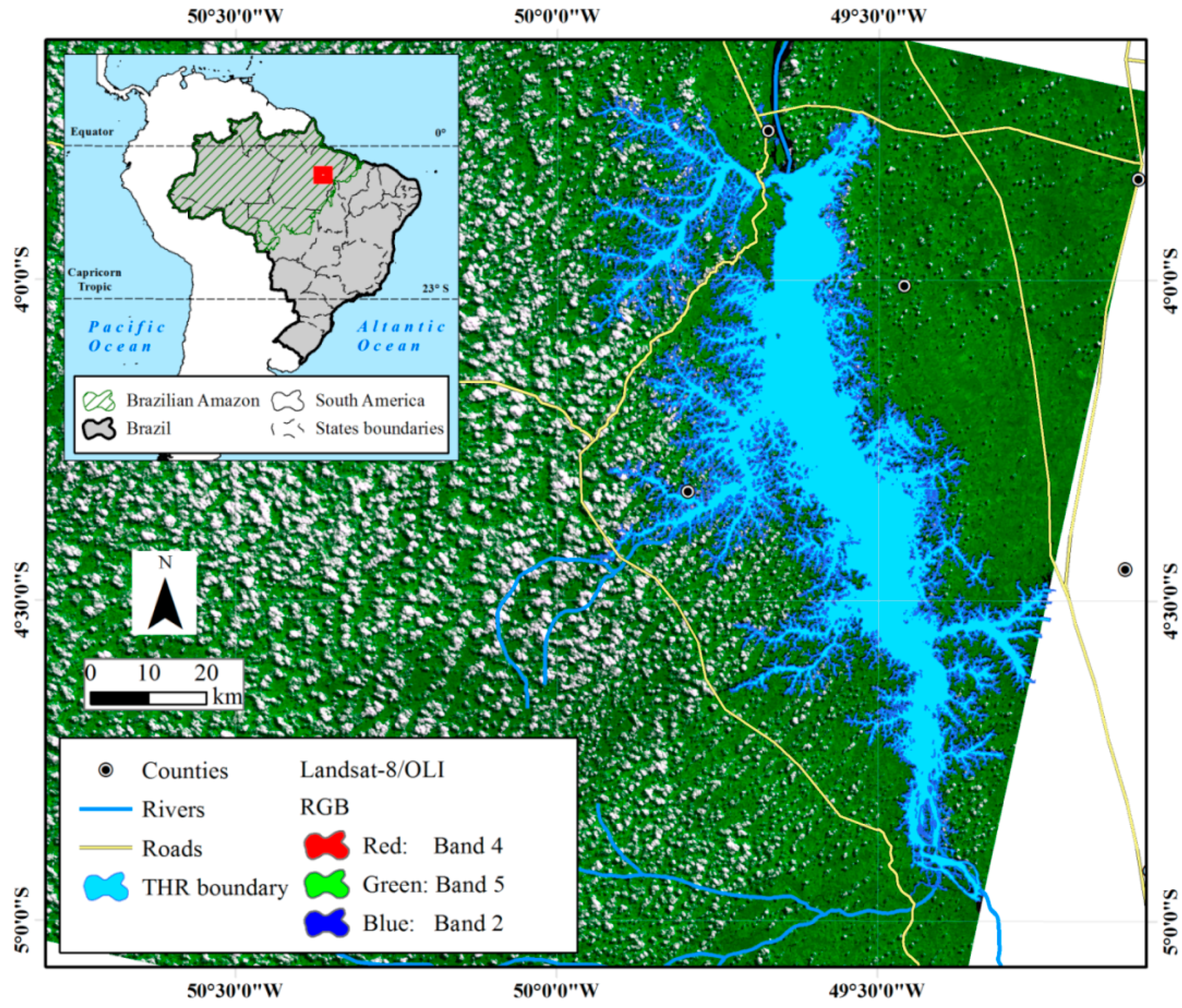
2.1. Study Area

The area selected for this study comprises the Tucuruí Hydroelectric Reservoir (THR), located between the coordinates 3.755°S; 49.528°W and 5.007°S; 49.587°W, Para State, Brazilian Amazon (Figure 1). This area encompasses parts of seven counties in the Southeastern Pará: Novo Jacundá, Novo Repartimento, Novo Breu Branco, Nova Ipixuna, Itupiranga, Goianésia do Pará and Tucuruí.
The THR was planned and constructed between 1960 and 1980 by the damming of the Tocantins River, flooding a vast area of the tropical rainforest [8]. The regional topography and morphology resulted in an elongated shape of the reservoir, from the north to the south, around 150 km in length and 20 km in width. The THR has a flooded area of 2918 km2 (water level 74 m above sea level), a total volume of 50.3 billion m3 [13] and a residence time around 51 days [14].
Figure 1. Study area: THR location at Brazilian Amazon.
Ijgi 04 00220 g001

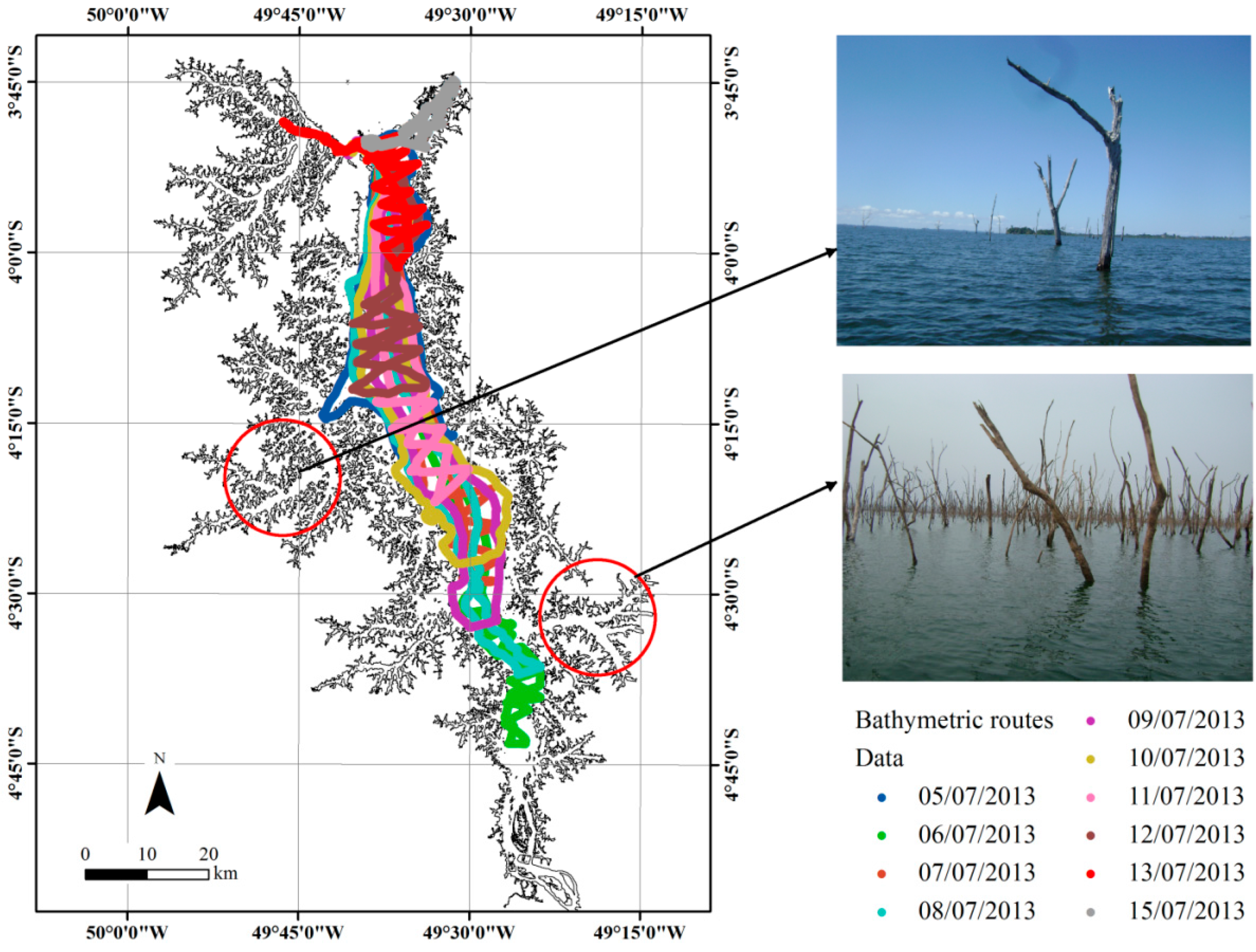
2.2. Depth Samples Dataset

The depth samples were collected during one field survey conducted in the THR from 3 to 16 July 2013. The choice of period for the execution of the field survey was based, among others factors, on the reservoir level which was near the maximum operational level during the field survey.
The bathymetric survey had two steps: (1) the planning and (2) the data collection. The bathymetric survey follows the protocols described by [15,16]. The planning of the field survey was performed using a Landsat-8 image, acquired by the sensor Operational Land Imager (OLI) [17], Google Earth® [18] and a Geographic Information System (GIS). These procedures had the objectives of optimizing the time and costs of the field survey, ensuring all regions of interest were sampled and redundant data collection. The routes were defined taking into account the large number of islands and dead trees in the reservoir, a fact that complicates and compromises the safety of navigation especially in conditions of moderate and strong winds. The total route planned for a day of work was defined taking into account an average travel speed of 20 km·h−1 and a maximum of 11 h worked on the same day (06:00 h–17:00 h). During the survey, the depth samples were collected using an ecobathymeter model GPSmap 520s Garmin® (Olathe, KS, USA). This ecobathymeter operates in two frequencies (50 Hz and 200 Hz) and has a vertical accuracy of ±0.1 m. The equipment was preprogrammed to collect and store depth samples every 2 s, using the geographical coordinate system and the World Geodetic System 1984 (WGS-84) as the datum. The bathymetric routes were stored in the ecobathymeter memory and used as a navigation reference during the data collection.

2.3. Interpolation Procedure

The interpolation procedure was conducted in the following way. First, the depth samples, containing the latitude, longitude and depth value, were exported from the internal memory of the ecobathymeter as a text file (.txt) using the MapSource® software. The preprocessing step was conducted using a Microsoft Excel spreadsheet and aimed to correct the depth samples before the spatial interpolation. We corrected the depth values to the maximum operational level (74 m above sea level) based on the reservoir level on the days of the field survey. The reservoir level is available online with a daily frequency by the company which operates the reservoir [19]. After the preprocessing step, an Exploratory Spatial Data Analysis (ESDA) [20] was conducted with the depth samples dataset. The ESDA was carried out using the ArcGIS® Geostatistical Analyst toolbar [21] and had the aim of examining the accuracy of the dataset, to detect anomalous behavior in the dataset, to test if the hypotheses assumed (e.g., normality) are valid and to detect outliers in the dataset before the spatial interpolation.
The spatial interpolation was conducted using four different interpolation methods (3 deterministic and 1 geostatistical), which are available in the ArcGIS® Geostatistical Analyst toolbar. The spatial interpolators assessed in this work were: IDW, Local Polynomial Interpolation (LPI), RBF and OK. Among them, the OK is the only geostatistical method. These methods were chosen because they are widely used in the literature [10,11,12] and are frequently used to interpolate bathymetric data in different aquatic systems [4,8,9].
The IDW is an exact interpolation method which estimates the depth values at unsampled points using a linear combination of values at sampled points weighted by an inverse function of the distance from the point of interest to the sampled points [10]. The assumption of this method is that sampled points closer to the unsampled point are more similar to it than those further away in their values. The LPI is an inexact interpolation method which estimates the depth values at unsampled points by fitting a specified order polynomial surface using all points only within a defined neighborhood [10]. The RBF is an exact interpolation method, conceptually similar to fitting a surface through the measured depth values while minimizing the total curvature of the surface; this method is indicated to calculate smooth surfaces from a large number of data points. Finally, the OK is a geostatistical method which is commonly used in environmental sciences to describe spatial patterns and interpolate the values of the primary variable at unsampled locations as well as model the uncertainty or error of the estimated surface [10]. During the OK interpolation, the semivariogram adjustment was done interactively, by changing the sill, range, lag and nugget values. The semivariogram was adjusted to model the spatial autocorrelation between the depth samples before applying the OK method.
For all the interpolation methods evaluated in this study, we tested different parameterizations and adjustments. For the IDW method, we tested different numbers of neighbors, length of semi-axis and power parameter. For the LPI method, we tested different polynomial orders and kernel functions. For the RBF method, we tested different numbers of neighbors, length of semi-axis and kernel functions. For the OK method, we tested different adjusts of the semivariogram. The best parameterization of each interpolation method was defined based on the cross-validation results. For the depth samples measured twice at the same longitude and latitude during the data collection, the ArcGIS® Geostatistical Analysis Toolbar offers the following option: use the maximum value, use the minimum value and use the mean value. We used the mean value in our application.
The validation of each spatial interpolation method was conducted using the cross-validation technique, a popular statistical technique used to evaluate interpolation methods [22]. In this case, we used the leave-one-out cross validation (LOOCV) implemented in ArcGIS® Geostatistical Analyst toolbar, which is a special case of k-fold cross validation. At each iteration of LOOCV, a single sample value was removed from the entire dataset, the interpolation algorithm was applied to the remaining dataset and after the interpolation, and the result was compared with the sample value removed from the entire dataset. This procedure was repeated n times (where n is the number of samples in the dataset), where we do not re-evaluate the interpolation method parameters during the LOOCV procedure. At the end of this procedure the bias, Mean Absolute Error (MAE), the Root-Mean-Squared-Error (RMSE) and the coefficient of determination (R2) were produced for each interpolation method, as described by [10]. Finally, these four spatial interpolation methods were compared based on RMSE using a Monte Carlo Simulation (MCS) [23]. The MCS was performed using the R statistical environment [24]. During each iteration of the MCS, random error values were drawn from each of the datasets, and the RMSE values were computed and stored. Respecting the central limit theorem, we used 10% of the total data for each dataset. The MCS was performed for 10,000 iterations. After the MCS, we conducted an ANOVA and Tukey statistical tests to verify if the simulated RMSE were statistically different from each other.

2.4. Information Extraction

The bathymetric grid obtained by the spatial interpolation method with the best performance was used to derive further information about the THR, such as level-area and level-volume diagrams. This information was generated using the ArcGIS® 3D Analyst toolbar [25] and a Microsoft Excel® spreadsheet. First, the reservoir surface area and volume was calculated using the Surface Volume tool in the ArcGIS® 3D Analyst toolbar. This tool calculates the area and volume of a raster, a triangulated irregular network (TIN), or a terrain dataset surface above or below a given reference plane. In our application we used the maximum reservoir water level (74 m above mean sea level) as the reference plane and calculated the surface area and volume at each 2 m depth below this plane. We then used the Excel® spreadsheet to correlate the surface area and volume with the water level and generate the level-area and level-volume diagrams. During the regression analysis the best-fit lines were adjusted using the least-squares method.

3. Results and Discussions

3.1. Depth Samples Dataset and Exploratory Analysis

During the field survey a total of 2017 km were traveled with a mean speed of 25 km·h−1, which corresponded to around 90 h of work. The reservoir area covered in the field survey corresponds to around 2600 km2 (~90% of total reservoir area). Due to the presence of dead trees, some shallow areas in the littoral zone could not be sampled during the survey. At the end of survey, a total of 179,898 depth samples were collected. Table 1 shows a statistical summary of the depth samples dataset while Figure 2 shows the bathymetric routes made during field survey.
Table 1. Statistical summary of the depth sample dataset.
Number of samplesMaximum Value (m)Minimum Value (m)Mean Value (m)Standard Deviation (m)
179,898107.50.538.216.7
Figure 2. Bathymetric routes conducted during the field survey. The red circles indicate the locations not sampled due to difficulty of access and the presence of many dead trees. The color code indicates the acquisition date.
Ijgi 04 00220 g002

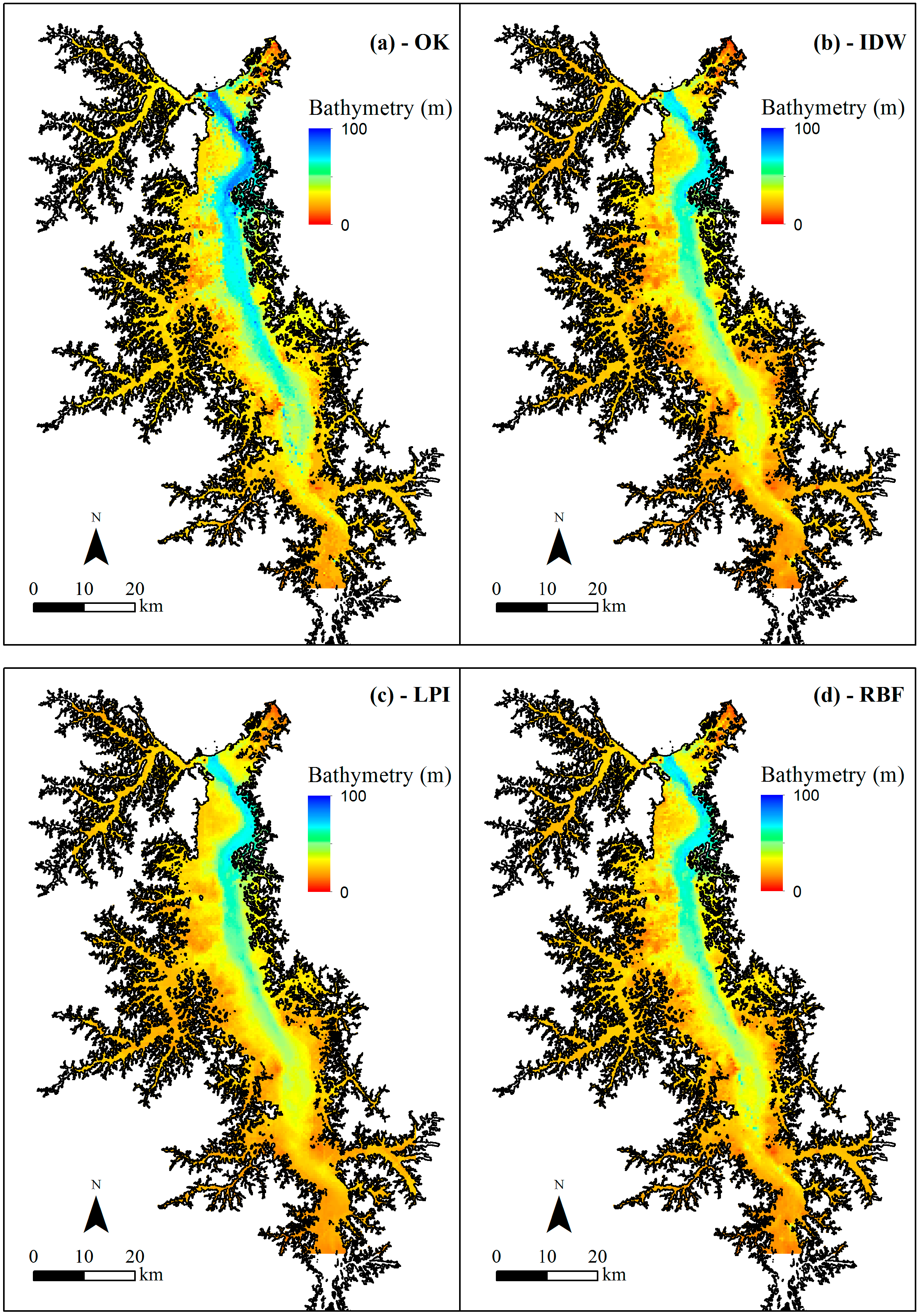
3.2. Comparison of Spatial Interpolation Approaches

Figure 3 shows the results of applying the four spatial interpolation methods to the depth samples dataset, with the parameterization that showed the best results for each method (Table 2). For all the four methods, the interpolated grid has a 250 m × 250 m spatial resolution.
Figure 3. Bathymetric grids obtained from the different spatial interpolation methods: (a) Ordinary Kriging—OK; (b) Inverse Distance Weighting—IDW; (c) Local Polynomial Interpolation—LPI; (d) Radial Basis Function—RBF.
Ijgi 04 00220 g003
Table 2. Summary of parameters used in the spatial interpolation methods.
MethodParameterization
OK *Neighbors = 25; length of semi-axis = 1300; lags = 12; lag size = 46; semivariogram = Stable
IDW **Neighbors = 40; length of semi-axis = 5000; power = 2
LPI ***Neighbors = 40; length of semi-axis = 5000; polynomial order = 2; kernel function = Constant
RBF ****Neighbors = 10; length of semi-axis = 5000; kernel function = Completely Regular Spline
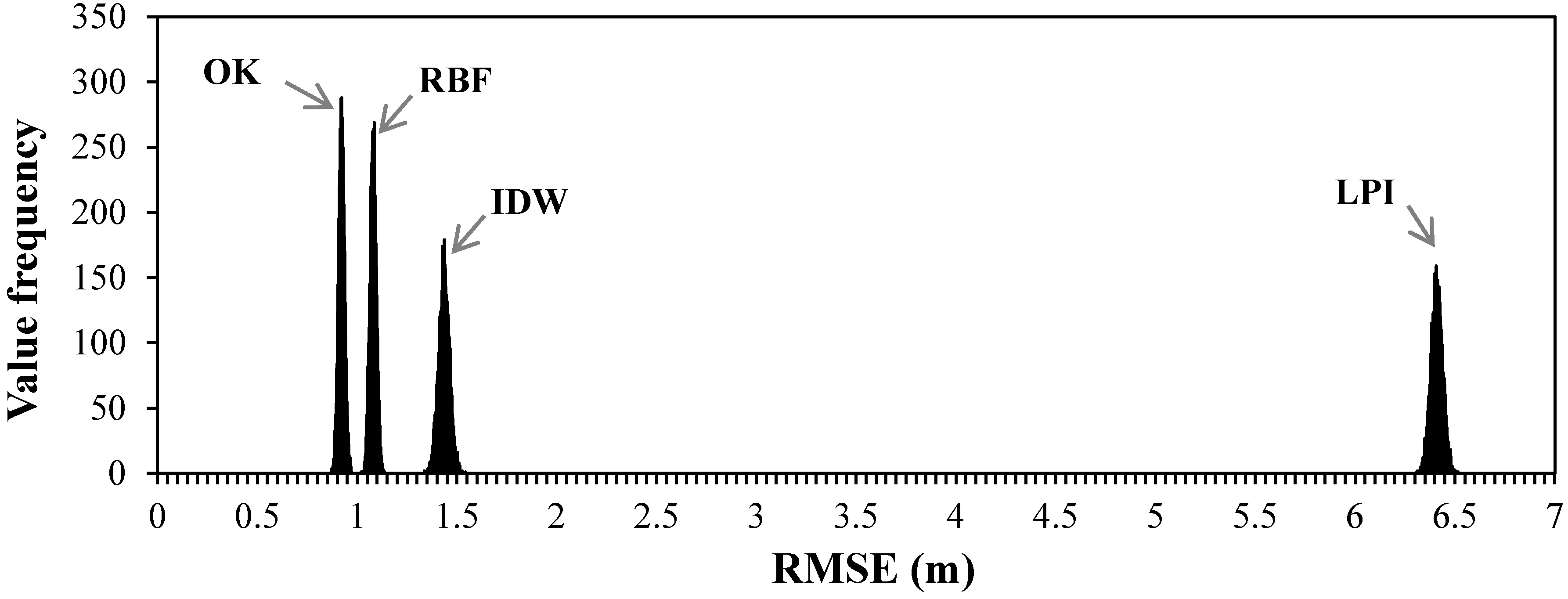
Note: * Ordinary Kriging (OK); ** Inverse Distance Weighting (IDW); *** Local Polynomial Interpolation (LPI) and **** Radial Basis Function (RBF).
All the resulting interpolated bathymetric grids had a similar depth range, going from approximately 0.5 m to 100 m depth with a mean value of around 28 m. The Tocantins River channel and the region near the dam showed higher depths compared with the littoral and transition zones. We also observed that most of submerged islands are present in the left bank of THR, where the flood plain is larger than on the right side of the bank. Qualitatively, all the four methods used to interpolate the depth samples yielded reliable results and were able to map important bathymetric features, such as the main channel of the Tocantins River and some submerged islands. This is important for 3-D hydrodynamic modeling studies, once the currents and the water circulation are induced by reservoir bathymetry [1].

3.3. LOOCV

Figure 4 and Table 3 show the results of the cross-validation procedure.
Figure 4. 2D color scatter-plot between measured and estimated depth values: (a) Ordinary Kriging—OK; (b) Inverse Distance Weighting—IDW; (c) Local Polynomial Interpolation—LPI; (d) Radial Basis Function—RBF. The color code indicates the absolute error range.
Ijgi 04 00220 g004
Among the four interpolation methods tested, the OK algorithm was the one with the lowest MAE (0.45 m or 0.42%) RMSE (0.92 m or 0.86%) and higher correlation with in situ measurements (R2 = 0.997) if compared to the other three methods used. On the other hand, the LPI algorithm was the one with the worst results, leading to a RMSE higher than 6 m (~6%) and a correlation coefficient of 0.85. The IDW and RBF methods showed results similar to the OK algorithm with an RMSE lower than 1.5 m (1.4%) and a correlation coefficient higher than 0.99. The LPI was the only algorithm that showed a general tendency to overestimate the depth (bias = 0.17 m); all the other three methods (OK, IDW and RBF) showed a slight tendency to underestimate the depths at THR (bias lower than 0.005 m).
Table 3. Summary of LOOCV analysis.
MethodBias (m)MAE (m)MAE (%)RMSE (m)RMSE (%)R2
OK *−0.0010.450.420.920.860.997
IDW **−0.0050.710.661.431.330.993
LPI ***0.1744.694.376.415.960.858
RBF ****−0.0020.520.481.081.000.996
Note: * Ordinary Kriging (OK); ** Inverse Distance Weighting (IDW); *** Local Polynomial Interpolation (LPI) and **** Radial Basis Function (RBF).
Except for the LPI method, all the other three methods evaluated in this study showed low RMSE values for 3D hydrodynamic modeling purposes. Taking the RMSE value of the OK method as a reference, the IDW, LPI and RBF methods showed RMSE values around 55%, 596% and 17% higher, respectively. The good performance of OK, IDW and RBF (RMSE < 5%) can be attributed to the high density of samples used; according to Li and Heap [10] geostatistical methods, such as OK, do not show significantly greater improvements in prediction than deterministic methods, such as IDW and RBF, for high density samples.
To compare with our study, similar results were found by Merwade et al. [8] and Bello–Pineda and Hernández–Stefanoni [9] when comparing different interpolation methods to generate a river channel and submerged platform bathymetric grids. In the two abovementioned studies, the geostatistical methods also presented a better performance when compared with other deterministic interpolation methods. For the river channel bathymetry [8] the OK method showed a mean RMSE value of 0.27 m while the IDW method showed a mean RMSE value of 0.54 m (i.e., 100% higher than the RMSE of the OK method). For the submerged platform bathymetry [9], the IDW method showed a RMSE about 20% to 30% higher than RMSE produced by OK method.
In order to analyze the spatial distribution of the errors (i.e., predicted–observed values) produced during the interpolation procedure, we generated error grids for each of the methods assessed (Figure 5). The error grids were generated using the error values produced during the LOOCV following the same spatial interpolation procedure described in Section 2.3. To compare the four error grids we reclassified them into four classes: (1) error < −1 m; (2) −1 m ≤ error ≤ 0 m; (3) 0 m < error ≤ 1 m; and (4) error > 1 m. Negative error values (classes 1 and 2) indicate an underestimation of depth values by the interpolation method while positive error values (classes 3 and 4) indicate an overestimation of the depth by the interpolation method.
Figure 5. Spatial distribution of error (m) classes for the different interpolation methods: (a) Ordinary Kriging—OK; (b) Inverse Distance Weighting—IDW; (c) Local Polynomial Interpolation—LPI; (d) Radial Basis Function—RBF.
Ijgi 04 00220 g005
From the spatial point view, the OK and RBF methods (Figure 5a,d) tended to underestimate the depth values in most of the grid cells while the IDW and LPI methods (Figure 5b,c) showed a tendency to overestimate the depth values in most of the grid cells. The OK method (Figure 5a) underestimated the depth values (classes 1 and 2) in 56% of the grid cells and overestimated the depth values (classes 3 and 4) in 44% of grid cells. The IDW method (Figure 5b) underestimated the depth values in 48% of the grid cells and overestimated the depth values in 52% of grid cells. The LPI method (Figure 5c) underestimated the depth values in 47% of the grid cells and overestimated the depth values in 53% of grid cells. The RBF method (Figure 5d) underestimated the depth values in 51% of the grid cells and overestimated the depth values in 49% of grid cells. The LPI was the only method that showed most of the grid cells classified into classes 1 and 4 (absolute error > 1 m), around 79% of cells. On the other hand, the OK, IDW and RBF methods showed more than 95% of the grid cells classified into classes 2 and 3 (absolute error < 1 m).
For the OK, IDW and RBF interpolation methods there were no clear pattern observed in the spatial distribution of the error, although the error tended to be higher (in absolute values) and more heterogeneous in the littoral zone and in some reservoir’s embayment than in the main body of the reservoir. This fact can be explained as a result of the low depth sample density collected in the shallow zones of the reservoir. Conversely, in the regions with a high depth sample density (e.g., the main body of the reservoir), the OK, IDW and RBF methods showed similar results and low error values (in absolute values). The LPI method showed a distinct pattern in the spatial distribution of error when compared to the other three analyzed methods. In this case, the errors produced by the LPI method were heterogeneous and high (in absolute values) in all distinct reservoir zones. Furthermore, the LPI method was the only one that tended to underestimate the depth values along the river channel.

3.4. Monte Carlo Simulation

In order to analyze if the RMSE obtained for each interpolation method was statistically different, we performed a MCS. Figure 6 shows the histograms of RMSE values simulated for each interpolation method. The RMSE simulated for the OK method ranged from 0.87 to 0.97 m with a mean value of 0.92 m while that of the IDW method ranged from 1.34 to 1.54 m with a mean value of 1.44 m. The RMSE simulated for the LPI method ranged from 6.31 to 6.51 m with mean value of 6.41 m while the RBF method ranged from a RMSE of 1.02 to 1.14 m with a mean value of 1.08 m. As can be noted, the mean RMSE simulated for the LPI method was more than 500% higher than the RMSE simulated for the other three methods. The RMSE simulated for the OK and RBF methods were similar with less than 18% difference.
Figure 6. Histograms showing the results of Monte Carlo Simulation.
Ijgi 04 00220 g006
To test whether the mean RMSE simulated was significantly different, we performed an ANOVA test (p-value < 0.001). The results of this test showed that at least one mean RMSE simulated was statistically different from the others (p-value < 0.01). An additional Tukey test showed that among the four spatial interpolation methods used in this work, the OK algorithm showed statistically lower RMSE (p-value < 0.001) when compared with the other three methods.
The best result yielded by the OK algorithm, compared to the other three methods tested, can be attributed to the geostatistical nature of this algorithm, which considers the spatial autocorrelation among the samples during the interpolation procedure [10]. Also, the OK method is recommended for data that are irregularly sampled, such as the dataset used in this study.

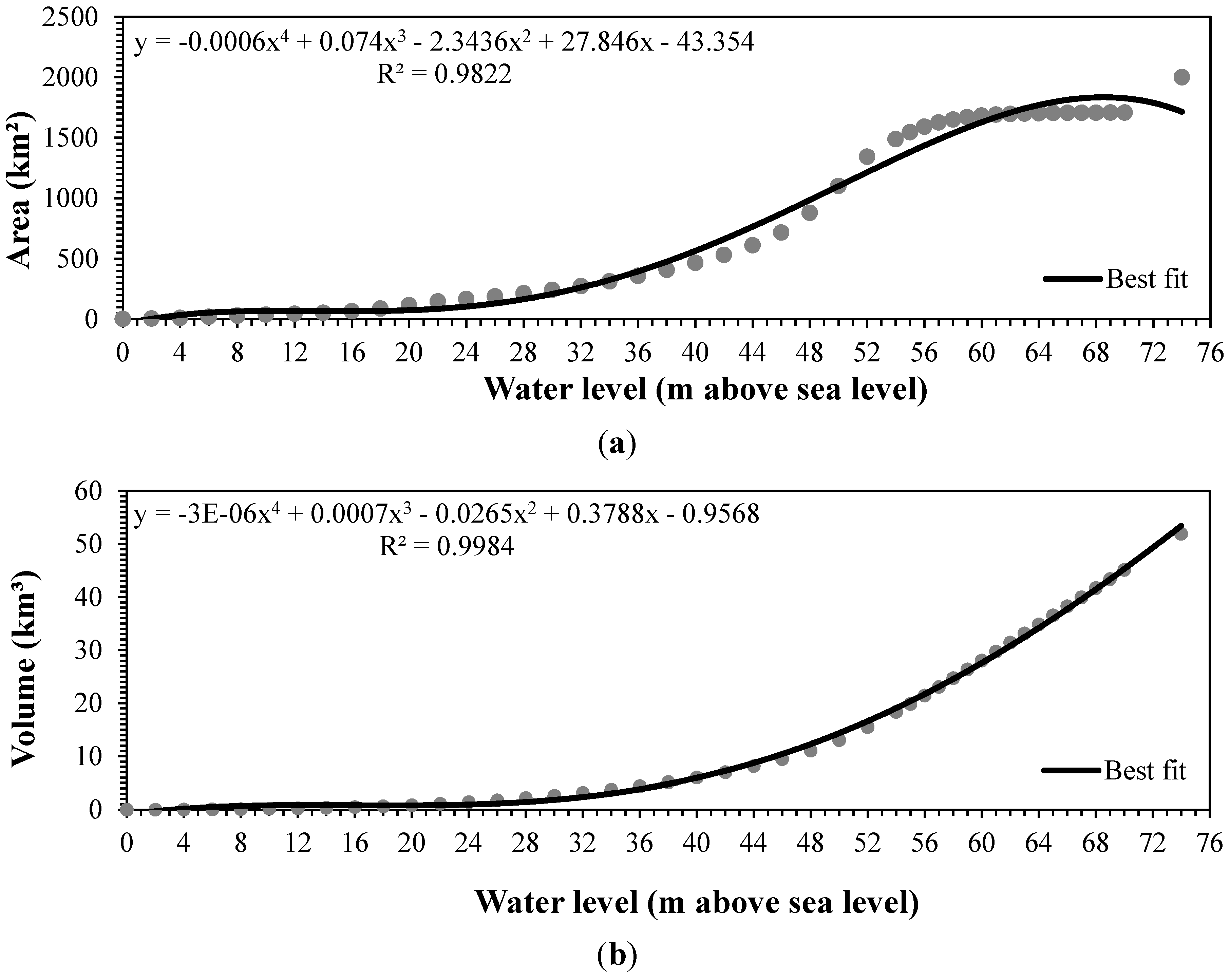
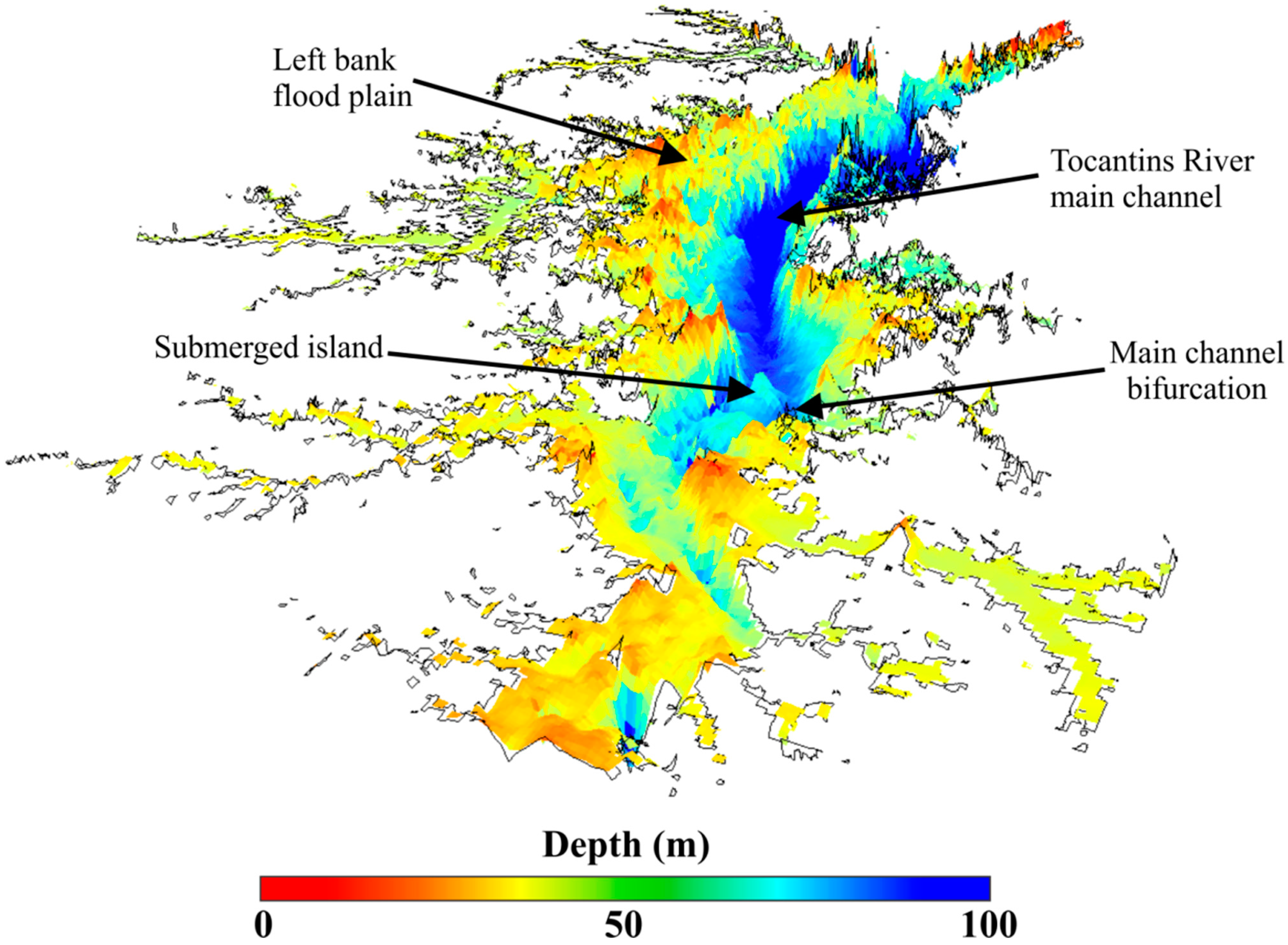
3.5. Examples of Information Extracted from the Bathymetric Grid

Using the bathymetric surface generated by the interpolation algorithm with the best performance and a GIS, it was possible to extract further information about the reservoir characteristics. This information can be used for the operational monitoring of the reservoir and also for hydrodynamic and water quality modeling studies. Figure 7 shows the level-area (Figure 7a) and level-volume (Figure 7b) diagram while Figure 8 shows the three-dimensional bathymetric view of the reservoir.
Figure 7. Information extracted from the bathymetric grid obtained from the OK method: (a) Level-area diagram; (b) Level-volume diagram.
Ijgi 04 00220 g007
For the THR the best fit for the two diagrams was obtained using a fourth order polynomial function (R2 > 0.96). Using these diagrams it is possible to optimize the operational monitoring of the THR, by estimating the reservoir area and volume as a function of water level, which is a variable that is easy to measure. These diagrams can be also used to monitor the reservoir generation capacity. We estimated the surface area and the total volume for the THR to be around 2100 km2 and 52 km3 (water level at 74 m above sea level), respectively.
Figure 8. Three-dimensional view of reservoir bathymetry.
Ijgi 04 00220 g008

4. Conclusions

In this study we assessed four spatial interpolation methods for mapping the bathymetry of an Amazonian reservoir. The main conclusions are:
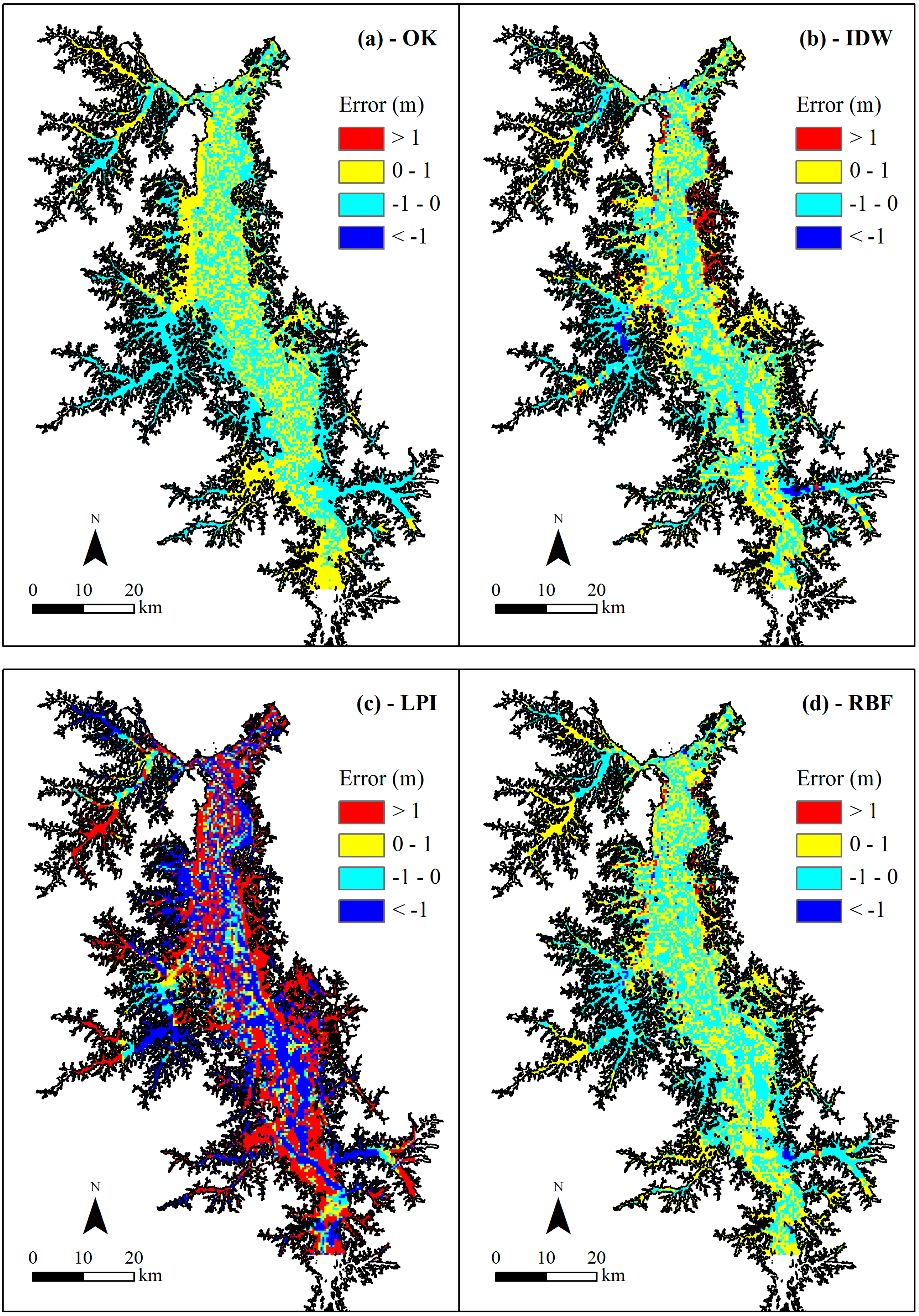
  • Qualitatively, all the four interpolation methods used in this work were able to map important bathymetric features in the THR, such as the Tucuruí River channel and the submerged island. Visually, all methods tested yielded similar results.
  • Quantitatively, and for this Amazonian reservoir case, the geostatistical method provided the best results, with the OK algorithm showing lower RMSE (0.92 m or 0.86% of range) and higher correlation coefficient (0.997) when compared to IDW, LPI and RBF algorithm. This may be due to the fact that the depth samples were irregularly spaced, where the OK method is better suited. Thus, choice of which method to use could be guided by the sample design.
  • The LPI algorithm has not been used very often in this context and showed a general tendency to overestimate the THR depths. The other three methods showed a slight tendency to underestimate the depth values.
  • From the spatial point view, the OK, IDW and RBF methods showed no clear pattern in the error distribution, although high error values (in absolute terms) occurred in the zones of the reservoir with low depth sample density (e.g., littoral and transition zones). In the zones of the reservoir with a high depth sample density, the OK, IDW and RBF methods showed a similar performance with low error values (in absolute terms).
  • The bathymetric grid obtained by the OK method was the most suitable for extract additional information about the THR. This information is crucial for reliable three-dimensional hydrodynamic and water quality modeling studies and for the operational monitoring of the Amazonian reservoir.
  • Future studies are required to determine whether these patterns are similar in other Amazonian reservoirs, i.e., whether a geostatistical approach provides the best solution for this problem domain.
  • Future studies should compare methods, which consider the anisotropic nature of riverbed and submerged relief, i.e., is the preferential direction of bathymetric data variability, during the interpolation procedure.

Acknowledgments

This work was supported by the “Instituto Nacional de Ciência e Tecnologia para Mudanças Climáticas” (INCT para Mudanças Climáticas, under grants CNPq 5737797/2008 and FAPESP 08/57719-9), the “Centrais Elétricas do Norte do Brasil S.A.” (ELETRONORTE, under grants ANEEL 4500075234) and Remote Sensing graduate program at the “Instituto Nacional de Pesquisas Espaciais” (DSR/INPE). The first author is grateful to the “Conselho Nacional de Desenvolvimento Científico e Tecnológico” (CNPq) for the doctorate scholarship (under grants 161233/2013-9). I.O. wishes to thank the “Coordenação de Aperfeiçoamento de Pessoal de Nível Superior” (CAPES) for the Masters scholarship. The authors are grateful to Mayko de Sousa Menezes for assisting with the bathymetric fieldwork and the Hidrosfera Research Group at DSR/INPE for the technical support.

Author Contributions

Marcelo Curtarelli is the main author who performed the analyses and wrote the paper with contributions from all the authors. Joaquim Leão and Marcelo Curtarelli collected the bathymetric data from the Tucuruí Reservoir. Igor Ogashawara and Joaquim Leão contributed to the spatial interpolation, the statistical tests and the Monte Carlo Simulation. João Lorenzzetti and José Stech designed the research as well as provided funding for the field trips.

Conflicts of Interest

The authors declare no conflict of interest.

References and Notes

  1. Imberger, J.; Hamblin, P.F. Dynamics of lakes, reservoirs, and cooling ponds. Ann. Rev. Fluid Mech. 1982, 14, 153–187. [Google Scholar] [CrossRef]
  2. Curtarelli, M.P.; Alcântara, E.H.; Rennó, C.D.; Assireu, A.T.; Bonnet, M.-P.; Stech, J.L. Modelling the surface circulation and thermal structure of a tropical reservoir using three-dimensional hydrodynamic lake model and remote-sensing data. Water Environ. J. 2013, 28, 516–525. [Google Scholar] [CrossRef]
  3. Bi, H.; Si, H. Numerical simulation of oil spill for the Three Gorges Reservoir in China. Water Environ. J. 2012, 28, 183–191. [Google Scholar] [CrossRef]
  4. Merwade, V. Effect of spatial trends on interpolation of river bathymetry. J. Hydrol. 2009, 371, 169–181. [Google Scholar] [CrossRef]
  5. Alcântara, E.; Novo, E.; Stech, J.; Assireu, A.; Nascimento, R.; Lorenzzetti, J.; Souza, A. Integrating historical topographic maps and SRTM data to derive the bathymetry of a tropical reservoir. J. Hydrol. 2010, 389, 311–316. [Google Scholar] [CrossRef]
  6. Gholamalifard, M.; Kutser, T.; Esmaili-Sari, A.; Abkar, A.A.; Naimi, B. Remotely sensed empirical modeling of bathymetry in the Southeastern Caspian Sea. Remote Sens. 2013, 5, 2746–2762. [Google Scholar] [CrossRef]
  7. Abileah, R.; Vignudelli, S. A completely remote sensing approach to monitoring reservoirs water volume. Int. Water Technol. J. 2011, 1, 63–77. [Google Scholar]
  8. Merwade, V.M.; Maidment, D.R.; Goff, J.A. Anisotropic considerations while interpolating river channel bathymetry. J. Hydrol. 2006, 331, 731–741. [Google Scholar] [CrossRef]
  9. Bello-Pineda, J.; Stefanoni-Hernández, J.L. Comparing the performance of two spatial interpolation methods for creating a digital bathymetric model of the Yucatan submerged platform. Pan-Am. J. Aquat. Sci. 2007, 2, 247–254. [Google Scholar]
  10. Li, J.; Heap, A.D. A Review of Spatial Interpolation Methods for Environmental Scientists; Geoscience Australia: Canberra, Australia, 2008. [Google Scholar]
  11. Azpurua, M.; dos Ramos, K. A comparison of spatial interpolation methods for estimation of average electromagnetic field magnitude. Prog. Electromagn. Res. M 2010, 14, 135–145. [Google Scholar] [CrossRef]
  12. Meng, Q.; Liu, Z.; Borders, B.E. Assessment of regression kriging for Spatial interpolation—Comparisons of seven GIS interpolation methods. Cartogr. Geogr. Inf. Sci. 2013, 40, 28–39. [Google Scholar] [CrossRef]
  13. Maciel, E.R. O Lago; Ética: Imperatriz, Brazil, 2012. (In Portuguese) [Google Scholar]
  14. Fearnside, P.M. Social impacts of Brazil’s Tucuruí dam. Environ. Manag. 1999, 24, 485–495. [Google Scholar] [CrossRef]
  15. Wilson, G.L.; Richards, J.M. Procedural Documentation and Accuracy Assessment of Bathymetric Maps and Area/Capacity Tables for Small Reservoirs; United States Geological Survey: Reston, VA, USA, 2006. [Google Scholar]
  16. Levec, F.; Skinner, A. Manual of Instructions: Bathymetric Surveys; Ministry of Natural Resources: Cochrane, ON, Canada, 2004. [Google Scholar]
  17. Irons, J.R.; Dwyer, J.L.; Barsi, J.A. The next Landsat satellite: The Landsat Data Continuity Mission. Remote Sens. Environ. 2012, 122, 11–21. [Google Scholar] [CrossRef]
  18. Google Earth. Available online: http://www.google.com/earth/ (accessed on 15 January 2014).
  19. Eletronorte—Tucuruí Operational Bulletin. Available online: http://www.eln.gov.br/opencms/opencms/pilares/geracao/estados/tucurui/ (accessed on 20 January 2014).
  20. Fotheringham, A.S.; Charlton, M. GIS and exploratory spatial data analysis: An overview of some research issues. Geogr. Syst. 1994, 1, 315–327. [Google Scholar]
  21. ArcGIS Geostatistical Analyst. Available online: http://www.esri.com/software/arcgis/extensions/geostatistical (accessed on 10 January 2014).
  22. Cressie, N.A.C. Statistics for Spatial Data; John Willey & Sons: New York, NY, USA, 1993. [Google Scholar]
  23. Liu, X.; Liu, Y.; Liu, H. Theory and Application of Monte Carlo Method; Springer: Heidelberg, Germany, 2012. [Google Scholar]
  24. R: A Language and Environment for Statistical Computing. Available online: http://www.r-project.org/ (accessed on 5 January 2014).
  25. ArcGIS 3D Analyst. Available online: http://www.esri.com/software/arcgis/extensions/3danalyst (accessed on 10 January 2014).

