Tracking 3D Moving Objects Based on GPS/IMU Navigation Solution, Laser Scanner Point Cloud and GIS Data

Abstract

Monitoring vehicular road traffic is a key component of any autonomous driving platform. Detecting moving objects, and tracking them, is crucial to navigating around objects and predicting their locations and trajectories. Laser sensors provide an excellent observation of the area around vehicles, but the point cloud of objects may be noisy, occluded, and prone to different errors. Consequently, object tracking is an open problem, especially for low-quality point clouds. This paper describes a pipeline to integrate various sensor data and prior information, such as a Geospatial Information System (GIS) map, to segment and track moving objects in a scene. We show that even a low-quality GIS map, such as OpenStreetMap (OSM), can improve the tracking accuracy, as well as decrease processing time. A bank of Kalman filters is used to track moving objects in a scene. In addition, we apply non-holonomic constraint to provide a better orientation estimation of moving objects. The results show that moving objects can be correctly detected, and accurately tracked, over time, based on modest quality Light Detection And Ranging (LiDAR) data, a coarse GIS map, and a fairly accurate Global Positioning System (GPS) and Inertial Measurement Unit (IMU) navigation solution.

1. Introduction

Rapidly developing sensor technologies provide increasingly rich data that can be processed by improving data fusion techniques, resulting in highly accurate multiple sensor integration that can effectively support high-level computer vision and robotics tasks, such as autonomous driving and scene understanding. Road traffic monitoring is a key component of autonomous driving and can be divided into subcategories, such as object segmentation, object tracking, and object recognition.

The progress in image and point cloud processing algorithms has resulted in stronger object tracking approaches. However, image and point cloud are prone to noise, clutter, and occlusion, and, thus, tracking still remains a challenging task in autonomous driving. In addition, a point cloud may be sparse, especially for inexpensive laser scanners, and motion of the platform may introduce a systematic error in the collected point cloud. This paper focuses on point cloud processing since image-processing algorithms are generally less reliable for autonomous vehicles.

Many papers, focused on the tracking of an object in the point cloud or image, ignore motion of the platform, which should be estimated to find/locate moving objects. There are some algorithms that discriminate moving objects and static objects in images [1], but these are not reliable for critical applications, such as traffic monitoring. Therefore, the motion of the platform should be measured using external sensors, such as the integration of Global Positioning System (GPS) and Inertial Measurement Unit (IMU) (also known as GPS/IMU), forming a navigation solution. The use of a GPS/IMU navigation solution enables the transfer of local laser scanner data to the global coordinate system and allows the use of prior information, such as Geospatial Information System (GIS) maps.

If an object is properly tracked and the pose of the object is estimated, an estimator, such as Kalman filter can be used to predict motion of the object and, consequently, proper actions can be taken to prevent potential risks. The success rate of the object tracking mainly depends on the accuracy of the pose estimation and the efficiency of the estimator. Since the pose estimation algorithms are sensitive to rigidity assumption of objects, and may deteriorate in the presence of noise and occlusion, the estimator may become unstable and diverge from the correct solution. Therefore, we propose a simple Kalman filter, which is more resilient to instability, and non-holonomic constraint, which is used to estimate the orientation of objects.

The paper is organized as follows: Previous works are addressed in Section 2. Section 3 describes prior information, which includes the lever-arm and boresight of sensors and GIS maps. The pipeline of point cloud processing is discussed in Section 4. The experiments are explained in Section 5, followed by results in Section 6, and conclusions in Section 7.

2. Literature Review

Tracking an object in images (also known as two-dimensional tracking) has been one of the most interesting research areas in computer vision. The widely known successful tracking approaches are face tracking [2,3] and histogram of gradient (HOG)-based pedestrian tracking [4]. However, 3D tracking has recently become a new focus of research. Three-dimensional (3D) tracking of objects became feasible using scene flow in images. Scene flow combines stereo matching and optical flow to estimate the 3D motion of the pixels in a scene [5,6,7]. However, scene flow is still not reliable for critical applications, and researchers continue working on improving the results of scene flow algorithms.

Three-dimensional tracking using a point cloud has recently attracted a great deal of research endeavors. Some of the approaches focus on better pose estimation, based on two consecutive epochs. The generalized Iterative Closest Point (ICP) is proposed to overcome the corresponding point assumptions of ICP [8]. If the color (or brightness) information is available, it can be used to improve point matching in two point clouds [9]. There are also many descriptors, developed to match the interest points in point clouds, which can be used to estimate the initial pose and refine the pose using ICP (or its variants) [10].

If the point cloud of an object is properly tracked over time and the points are accumulated, the point cloud becomes denser over time. This approach can be used to overcome the sparse point cloud problem, as well as the occlusion of an object. Newcombe et al. have implemented this approach for kinect data [11] and Held et al. have used this approach to track an object and accumulate points in a laser scanner point cloud [12,13].

The use of different estimators for 3D tracking has also been widely investigated. The Kalman filter is a popular estimator to track an object in robotics [14]. Ueda and his colleagues applied a particle filter to track an object. This approach is beneficial, especially for non-rigid objects, since the points are independently tracked [15]. Furthermore, different sensors can be integrated in order to improve the tracking. IMU data has been applied to improve pixel matching among images [16]. Radar, camera, and laser scanner data have been integrated in the Kalman filter to track moving objects in a scene [17]. A prototype of an autonomous vehicle, known as Google car, has been claimed to be fully operational [18]. However, this approach relies on high accuracy GIS maps, which are not affordable for most companies and institutions [19].

3. Prior Information

In this Section, required preprocessing steps are explained, including the coordinate system conversion and preparation of sensor information in the proper frames. In addition, GIS maps, such as OpenStreetMap (OSM), are described.

3.1. Geometric Model and Notation

For road traffic monitoring purposes, various sensors are mounted on the platform. GPS/IMU provides the position and orientation of the platform, independent from the objects in the scene, and then images and point cloud provide scene information, depending on the pose of the platform, and, finally, prior information (GIS maps) is used, which is independent from the traffic on the road.

All of these sensors and information sources have different frames (coordinate systems). The camera frame is located at the camera center and aligned in a way that the x and y coordinate axes are defined parallel to the image plane and the z coordinate axis is aligned along the principal axis of the camera toward the scene. The laser scanner frame is located at the center of its mirrors and its rotation axis defines its z-axis. The origin of IMU and its orientation depends on the IMU model. The origin of GPS is located at the phase center of the antenna and it does not have orientation. The GPS position is integrated with the IMU data, in order to obtain a near continuous and accurate navigation solution, and the GPS/IMU frame coincides with the IMU frame. GIS maps, retrieved from geospatial databases, have a global coordinate system.

In order to fuse multiple sensors, their individual frames should be transformed to a unified frame. The displacement vector and rotation matrix between sensor frames, independent from the pose of the platform, are called lever-arm and boresight, respectively. Here, we define a reference frame that is located at the IMU center at the first epoch of the data collection and it is aligned toward East, North, and Up (ENU), respectively. This frame has the orientation of the navigation frame, but unlike the navigation frame, it does not change with the platform motion. This in-house frame works fine locally, but should be redefined when the platform goes farther than a few hundred meters from the origin. The first epoch of data collection will be referred to as the reference epoch for the rest of this paper.

Each sensor’s data should be transformed to the reference frame. $C_{j,n}^{i,m}$ and $t_{j,n}^{i,m}$ are defined as the rotation matrix and displacement vector from frame i at time m into frame j at time n. The inertial frame is used to facilitate the transformation. The camera rotation from epoch k to the reference epoch, $C_{c,0}^{c,k}$ is given as follows:

$$C_{c,0}^{c,k}=C_{i,k}^{c,k}{C}_{inertial}^{i,k}{C}_{i,0}^{inertial}{C}_{c,0}^{i,0}$$

(1)

Superscripts and subscripts c and i stand for the camera and IMU frames and subscript 0 stands for the reference epoch. Obviously, $C_{i,k}^{c,k}= C_{i,0}^{c,0}$, and it is called boresight between the IMU and camera frames, assuming the platform is rigid and it should be estimated by calibration. $C_{inertial}^{i,k}$ and $C_{i,0}^{inertial}$ are the IMU measurements at epoch k and the reference epoch. The displacement vector between the camera frame at epoch k and the origin (IMU frame at the reference epoch) is given as follows:

$$t_{i,0}^{c,k}=C_{i,k}^{c,k}\left(t_{inertial}^{i,k}-t_{\text{i}nertial}^{i,0}\right)+C_{c,0}^{c,k}{t}_{i,0}^{c,0}$$

(2)

$t_{i,0}^{c,0}$ is lever-arm between the IMU and camera origins (camera position with respect to the IMU frame at the reference epoch) and is estimated from the calibration process. $t_{inertial}^{i,k}$ and $t_{inertial}^{i,0}$ are the displacement vector of the IMU frame at epoch k and the reference epoch with respect to the inertial frame and can be estimated from the GPS/IMU navigation solution. Obviously, the laser scanner frame and prior information can be transformed into the reference frame in the same way.

3.2. GIS Information

The advancements in satellite imagery, exploited by Internet mapping, such as Google Maps, resulted in easy production and access to map information worldwide. These maps are available in a rasterized format, contain the intensity or color information of pixels, and can be processed and converted into vector maps. Vector maps are stored in topological data structures that typically include point, line, and polygon features. We use vector maps since they are more flexible for spatial analysis and queries. These maps can be used as prior information and static objects in the scene may be located from the maps. From the road traffic monitoring and geospatial information perspective, roads, road signs, and traffic related information, such as crossings, are critical for our study.

OpenStreetMap (OSM) is a publicly available open source geospatial database under the Open Database License (ODbL) [20]. OSM’s data format follows Open Geospatial Consortium (OGC) standards [20]. Additionally, the geometric information of each feature is associated with some attributes, stored in a relational database. OSM data is accessible from OpenStreetMap or from various GIS softwares. Figure 1 shows the OSM road layer of the test area in ArcGIS.

Figure 1. The road centerlines retrieved from OSM and overlaid on the map. The roads are represented with the centerline (violet line).

Figure 1. The road centerlines retrieved from OSM and overlaid on the map. The roads are represented with the centerline (violet line).

GIS information content is always limited to a certain level of details, and the accuracy of its map is restricted to its registration. OSM road information, which is a line feature, contains only the centerline of the roads. In order to find whether an object is on the road, a buffer of the centerline is created and the road space is considered as the region of interest. The buffer size depends on the number of the lanes of a road, which is not stated in the database, and a certain number of lanes should be assumed. This assumption should be designed in the way that moving objects do not filter out.

4. Methodology

Road traffic monitoring can be divided into object segmentation, object tacking, and object recognition. In order to segment the objects, the point cloud should be refined and the outliers and the points that are not informative should be removed. The Euclidean clustering approach is used to segment the point cloud in a scene. The segmented point cloud includes static or moving objects. In order to understand road traffic, moving objects should be detected and the dynamics of their motion should be estimated over time. In order to accomplish moving objects discrimination, two segmented point clouds in two consecutive epochs are matched. The matching clusters are used to estimate the pose of objects between two epochs and an estimation filter is used to suppress noise in the estimated pose.

4.1. Object Segmentation

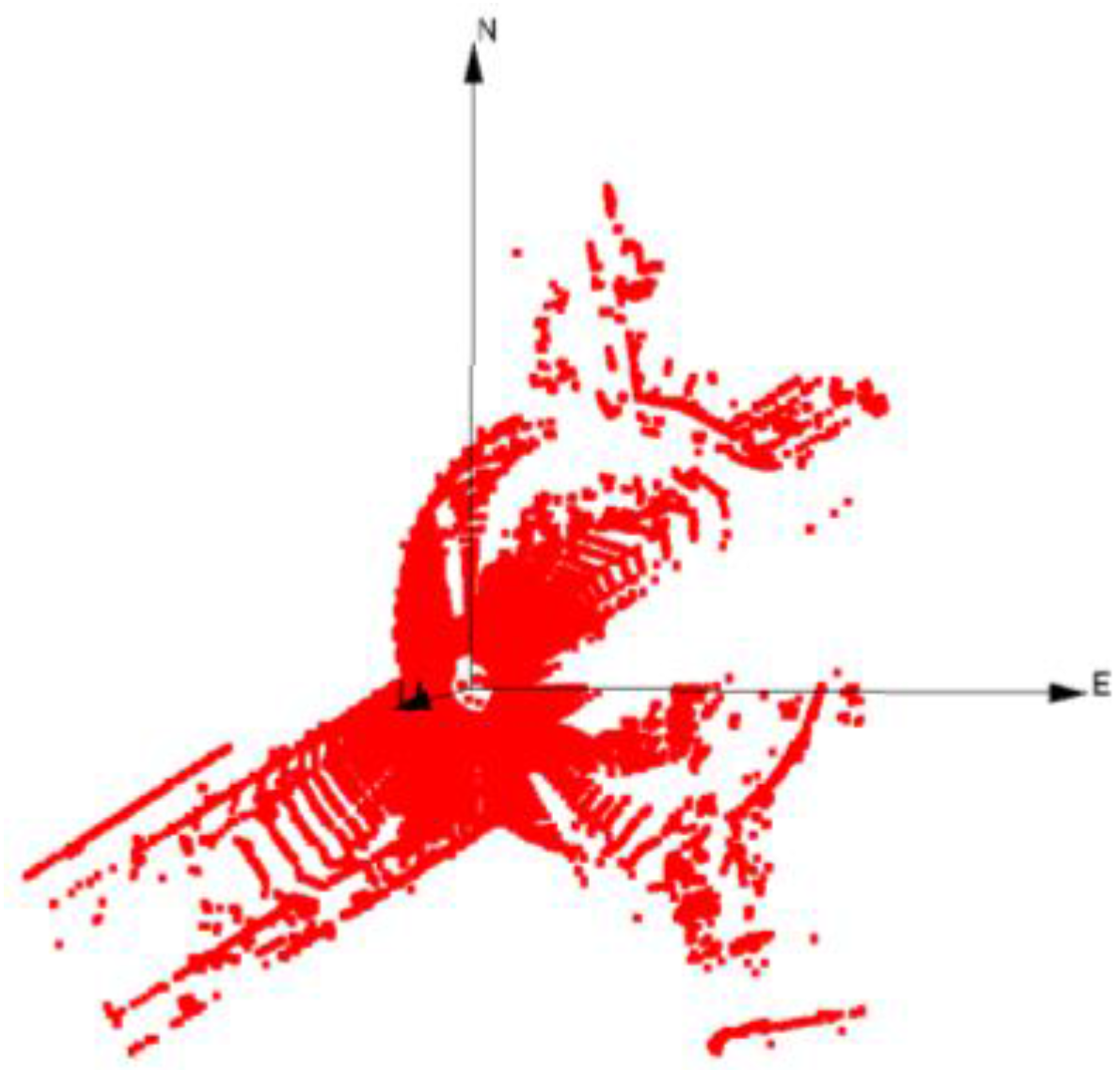
In order to track objects in a scene, it is necessary to detect objects in the point cloud. The point cloud, primary data source for our tracking method, is calculated based on time of flight of the laser beam emitted from the laser sensor, and detected at the laser scanner after reflected back from the surface of objects. Since a point cloud is a sampling of the surface of nearby objects from the laser scanner’s perspective, it is usually partially occluded. The measured 3D points should be transformed to the reference frame and should be independent from the pose of the platform. A point cloud collected from a laser scanner is shown in Figure 2. It should be noted that the motion of nearby objects and the platform might introduce a systematic error in the collected point cloud.

Figure 2. Laser scanner point cloud at one epoch in the reference frame (top view).

Figure 2. Laser scanner point cloud at one epoch in the reference frame (top view).

A point cloud contains 360° by 40° field of view (FOV) information, which is not needed in its entirety for road traffic monitoring and object tracking. Hence, we restrict our interest to the forward-looking points, as they provide the road traffic information ahead of the platform and overlap with forward-looking images. This overlap enables the coloring of a point cloud and the use of the color information in conjunction with the geometry information.

Many of the points in the point cloud fall on the ground and are less informative for our purposes. These points are eliminated from the point cloud using a plane fitting. Additionally, the points on the facade of buildings are not useful for object tracking and should be removed from the point cloud. The road space can be generated from geospatial database and is used to filter out the points off the road. After the filtering procedure, the point cloud has significantly fewer points and, therefore, considerably speeds up the point cloud processing. The three steps of point cloud filtering are shown in Figure 3.

Figure 3. Point cloud filtering: (a) The forward point cloud is kept and the rest is removed from point cloud; (b) the points on the ground are eliminated (grey); (c) the points off the road are excluded (dark green).

Figure 3. Point cloud filtering: (a) The forward point cloud is kept and the rest is removed from point cloud; (b) the points on the ground are eliminated (grey); (c) the points off the road are excluded (dark green).

There are many ways to segment objects in a filtered point cloud, including region growing [21], min-cut graph [22], difference of normal [23], and Euclidean distance based clustering. Here, we use the clustering based on the Euclidean distance, which clusters the connected components. The choice of threshold for the connected components is crucial. If the selected threshold is too high, it results in over-segmentation, if the threshold is too low, the opposite happens. Each cluster indicates an object and clustering can be considered as object segmentation. In Figure 4, each cluster is shown with a unique color.

Figure 4. Clusters in the scene are calculated based on Euclidean distance.

Figure 4. Clusters in the scene are calculated based on Euclidean distance.

Some of the segmented objects may not be interesting. For instance, the small objects may be road traffic signs and large objects may be buildings that have not been removed. Similarly, short objects may be vegetation and tall objects can be trees. Therefore, a filter is used to restrict the height and the footprint of objects.

4.2. Object Matching

If the laser scanner collects two point clouds in two consecutive epochs and each point cloud is filtered and segmented, there will be two sets of objects in a scene. If an object is observed in two epochs, the points in the clustered point cloud can be matched. Since the platform and objects are moving, the clustered point clouds of objects may not be identical in two epochs. The point clouds of an object in two consecutive epochs can be very different if an object is close to the sensor or not rigid, for example, different parts of the object may move independently.

In order to match the points of an object in two consecutive epochs, it can be assumed that the object does not move too fast and the location of the object in the previous epoch is close to its current location. While this assumption works fine in many cases, it may cause an error when there are multiple objects close to each other. We replace this assumption with the assumption that motion of the object is not abrupt and the predicted location of the object is close to its current measured location. Obviously, it needs an estimation filter to predict the position of the object, based on its dynamic model. While the use of an estimation filter improves the object matching, it does not guarantee that objects are matched correctly. Therefore, we allow an object to match to multiple objects in the previous epoch. In pose estimation, where the shape and color cues are used, we reject the objects that are not similar or have different colors.

4.3. Pose Estimation of Objects

When a corresponding object is found at two epochs, the displacement vector and rotation matrix of the object between two epochs can be estimated. The pose estimation is still a challenge since objects are (partially) self-occluded when they are seen from the laser scanner perspective. Additionally, point cloud may be noisy and cluttered and it may be prone to systematic errors. For instance, the platform motion may introduce a systematic error to the point clouds.

The most popular pose estimation algorithm is Iterative Closest Point (ICP), which minimizes the distance between the points of the matched objects. If $X_i\in o_m$ is the points on the surface of object $o_m$ and $X_j\in o_n$ are the points on the surface of object $o_n$ and these points are corresponding points in two consecutive epochs, then:

$$\underset{R,T}{\min }{\displaystyle \sum }_{X_i}\left|\left|\left(R{X}_i+T-X_j\right)n_i\right|\right|$$

(3)

where T and R are the translation vector and rotation matrix between two point sets and $n_i$ is the normal vector to the surface at point $X_i$. The solution to this minimization is calculated based on steepest descent in an iterative scheme. The assumption for ICP is the rigidity of the objects that may be violated if the objects are cyclist or pedestrian. When the occlusion is severe, ICP may fail to estimate the pose, even for rigid objects, such as cars. Additionally, the points are noisy and point $X_i$ and point $X_j$ may not be corresponding. Furthermore, ICP is prone to local minimum, and the approximate values of the rotation and translation between two point clouds should be known to converge to global minimum.

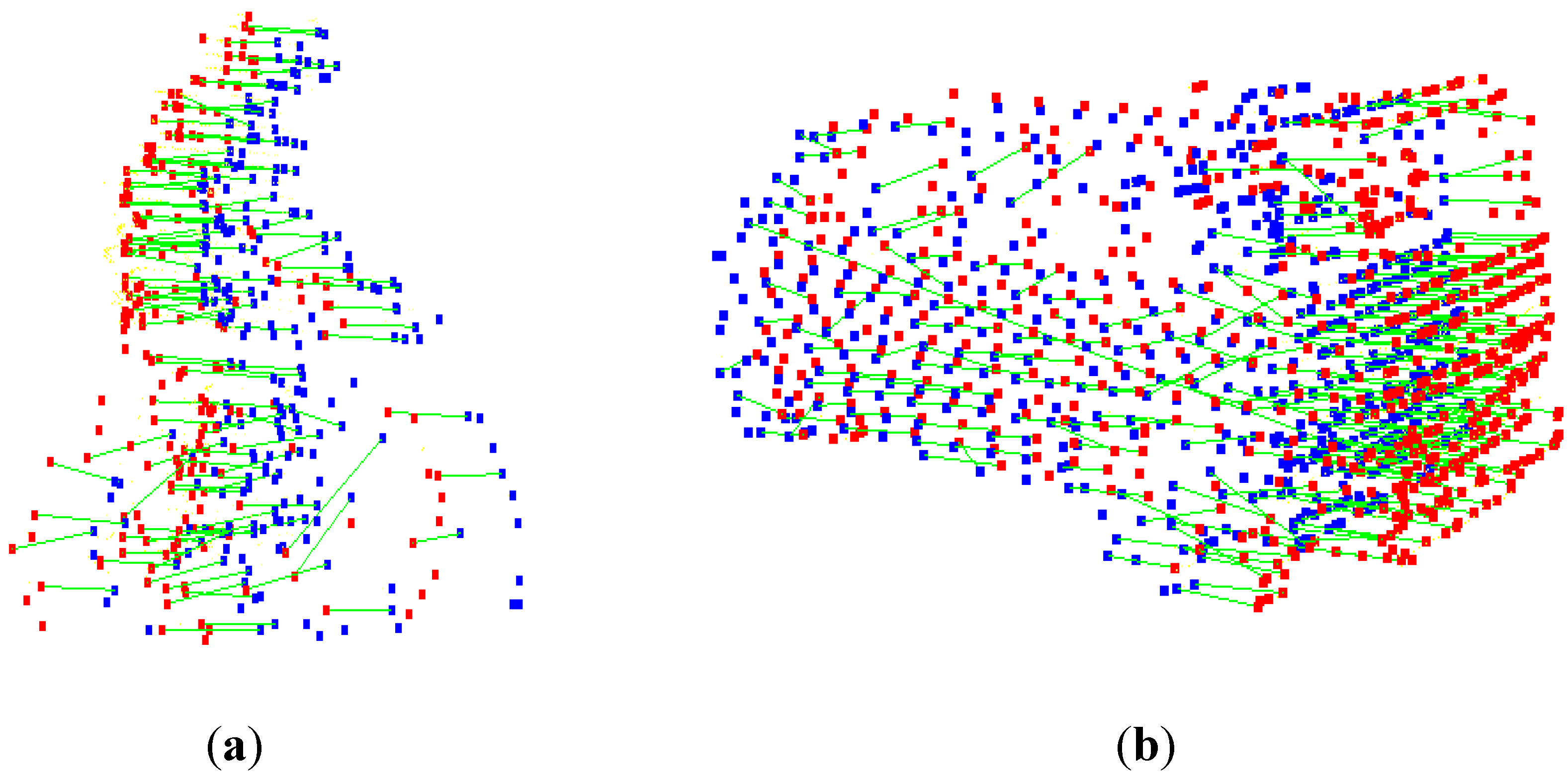
Another method, which is more resilient to the rigidity assumption, is feature matching. Like the salient points in images, and the salient points in point clouds are selected based on their uniqueness. These salient points are called features, and are described by the histogram of the curvature and surface, normal at that point, and its neighborhood, and is called the descriptor. If two descriptors are similar, the salient points are matched and the pose is estimated using matched points. Unfortunately, the object rigidity assumption is needed to define the descriptors, match them, and estimate the pose of the object. In addition to the rigidity assumption, the object may not have many salient points and the salient points may be incorrectly matched. Two examples of 3D feature matching are shown in Figure 5. It should be noted that the matching results are not always as good as of these examples.

There are some extensions to ICP that improve the results. Generalized ICP attempts to minimize the distance between two sets of points and their normal vectors. In contrast to ICP, which minimizes the distance between points, it is based on the minimization of the distance between planes [8]. Color supported generalized ICP uses the color consistency assumption between two epochs. In this method, the distance between two points in the point sets is replaced with a geometric and color distance, such that $d=\sqrt{{\left(X_i-X_j\right)}^T\left(X_i-X_j\right)+{\left(C_i-C_j\right)}^T\left(C_i-C_j\right)}$, where $C_i$ is color information [9]. In order to transfer the color to points, the projection matrix, $P$, is used. The point $X_i$ in point set is projected into image $x_i=P{X}_i$, where $x_i$ is the projected point into image space and the color content of the closest pixel in image is assigned to the point.

In a simplistic approach, the centroid of a matched object can be used to estimate the displacement vector between two epochs. However, it still suffers from the partially occluded geometry of the object. Since the centroid is used, the shape of the objects is neglected and the orientation cannot be estimated. Assumptions, such as non-holonomic assumption for the motion of the object, are required to estimate the orientation of the object between two epochs. It is obvious that this assumption fails when the object have lateral motion or make a sudden turn.

Figure 5. Feature matching: (a) A cyclist; (b) a car at two consecutive epochs (red and blue). Green lines represent the matched features.

Figure 5. Feature matching: (a) A cyclist; (b) a car at two consecutive epochs (red and blue). Green lines represent the matched features.

4.4. Object Tracking

In order to reduce noise in tracking and handle complete occlusions, we apply a bank of Kalman filters. Each Kalman filter estimates the pose of an object in a scene. If an object appears for the first time, a Kalman filter is added to the bank of Kalman filters, and its state vector is initialized. The position of the object is assumed at the centroid of the point set and its velocity is assumed to be zero. In other words, all of the objects in a scene are initially assumed to be static. The orientation of the object (yaw angle) is assumed to be in the direction of its velocity. Therefore, it is assumed that the object moves forward and the motion of the object in the scene is restricted to the motion on the ground plane.

We have applied Newton’s laws of motion to estimate the dynamics of the object’s motion. Based on these laws, the position can be estimated based on the velocity and acceleration, and velocity can be estimated based on acceleration. Therefore, Newton’s laws of motion can be written such that:

$$E_k=E_{k-1}+V_{E,k-1}\text{Δ}t+\frac{1}{2}{a}_{E,k-1}\text{Δ}{t}^2$$

(4)

$$N_k=N_{k-1}+V_{N,k-1}\text{Δ}t+\frac{1}{2}{a}_{N,k-1}\text{Δ}{t}^2$$

(5)

$$V_{E,k}=V_{E,k-1}+a_{E,k-1}\text{Δ}t$$

(6)

$$V_{N,k}=V_{N,k-1}+a_{N,k-1}\text{Δ}t$$

(7)

Additionally, azimuth can be estimated based on non-holonomic constraint.

$$Az=t{g}^{-1}\left(\frac{V_E}{V_N}\right)$$

(8)

Note that the Kalman filter can have more unknowns, but the more complicated dynamic model may diverge the results since the observations are highly noisy and unreliable. Here, the state vector is chosen such that:

$$x={\left[\begin{array}{ccc}E& N& \begin{array}{cc}{V}_E& V_N\end{array}\end{array}\right]}^T$$

(9)

The dynamic model of the Kalman filter is written such that:

$$x_k={\text{Φ}}_{k-1,k}{x}_{k-1}+G_k{\mu }_k$$

(10)

where ${\text{Φ}}_{k-1,k}$ is the state-transition matrix between epoch k-1 and epoch k, $G_k$ is a matrix relating system noise to the state vector and ${\mu }_k$ is system noise at epoch k. Here, we assume that the velocity is a random walk process, i.e., there is equal likelihood to increase or decrease the speed. The dynamic model of the object depends on its type. In other words, the dynamic model of pedestrian is different from the dynamic model of a vehicle, and the Kalman filter adaption is not trivial without knowing the object’s type.

$${\left[\begin{array}{c}E\\ N\\ V_E\\ V_N\end{array}\right]}_k=\left[\begin{array}{cccc}1& 0& \Delta t& 0\\ 0& 1& 0& \Delta t\\ 0& 0& 1& 0\\ 0& 0& 0& 1\end{array}\right]{\left[\begin{array}{c}E\\ N\\ V_E\\ V_N\end{array}\right]}_{k-1}+\left[\begin{array}{c}\frac{\Delta t^2}{2}\\ \frac{\Delta t^2}{2}\\ \Delta t\\ \Delta t\end{array}\right][w_a]$$

(11)

where $w_a$ is system noise assuming that velocity is the random walk process and $\text{Δ}t$ is the time span between two epochs. The observation model of Kalman filter is written such that:

$$z_{\text{k}}=H_k{x}_k+{\upsilon }_k$$

(12)

where $z_k$ is the observation vector, $H_k$ is the matrix relating the observation with the state vector and ${\upsilon }_k$ is noise of the observation at epoch k. Here, we use the centroid of the point set of an object ${\left[{\text{c}}_E,{\text{c}}_N\right]}^T$ to update the state vector such that:

$${\left[\begin{array}{c}{\text{c}}_E\\ {\text{c}}_N\end{array}\right]}_k=\left[\begin{array}{cccc}1& 0& 0& 0\\ 0& 1& 0& 0\end{array}\right]{\left[\begin{array}{c}E\\ \begin{array}{c}N\\ V_E\\ V_N\end{array}\end{array}\right]}_k+{\left[\begin{array}{c}{\epsilon }_{\text{E}}\\ \begin{array}{c}{\epsilon }_{\text{N}}\end{array}\end{array}\right]}_k$$

(13)

where ${\epsilon }_{\text{E}}$ and ${\epsilon }_{\text{N}}$ are noise of the observation. We have tested a more complex Kalman filters with more parameters in their state vector and used different pose estimation algorithms, but we found this simplistic approach the most efficient and reliable one.

4.5. Error Sources

The use of multiple sensors could provide a robust tracking solution, but the noise and systematic errors of each sensor may deteriorate the final results. Laser scanner data may be noisy, cluttered and prone to systematic errors. When the platform and objects are moving, the point cloud may be shifted. Additionally, the range error of the laser scanner can be significant. Since the laser does not exactly hit the same point in different epochs, porous objects, such as trees, can be very different in two epochs. The occlusion can cause incomplete perception of objects. Images are also prone to noise, systematic errors, and occlusion. The motion blur effect can be significant in moving platforms. In addition, most of image processing algorithms fail in the regions without texture.

GPS has a key role in our tracking pipeline. It provides the position of the platform with respect to the global coordinate system. The use of GIS maps depends on the position, which is estimated by GPS. In addition, in order to find moving objects, the motion of the platform should be observed by GPS and should be removed from observation. The accuracy of GPS positioning depends on the applied technology, as well as the signal reception in the area. If the carrier phase observation is used, its accuracy is within a few centimeters. If a standalone GPS technology is used, its accuracy may exceed a few meters. In addition, the signal blockage and multipath error may occur in an urban environment, which adversely affect the positioning accuracy. IMU sensors can be used to estimate the position and orientation of the platform in the absence of GPS. However, IMU is prone to noise, bias, and scale factor errors, and its accuracy quickly deteriorates over time, especially inexpensive IMUs. In the absence of GPS, static objects may be separated from moving objects in images and laser scanner data, and static objects may be used to estimate the position and orientation of the platform. The positioning of the platform in an urban environment during GPS signal blockage is an open problem.

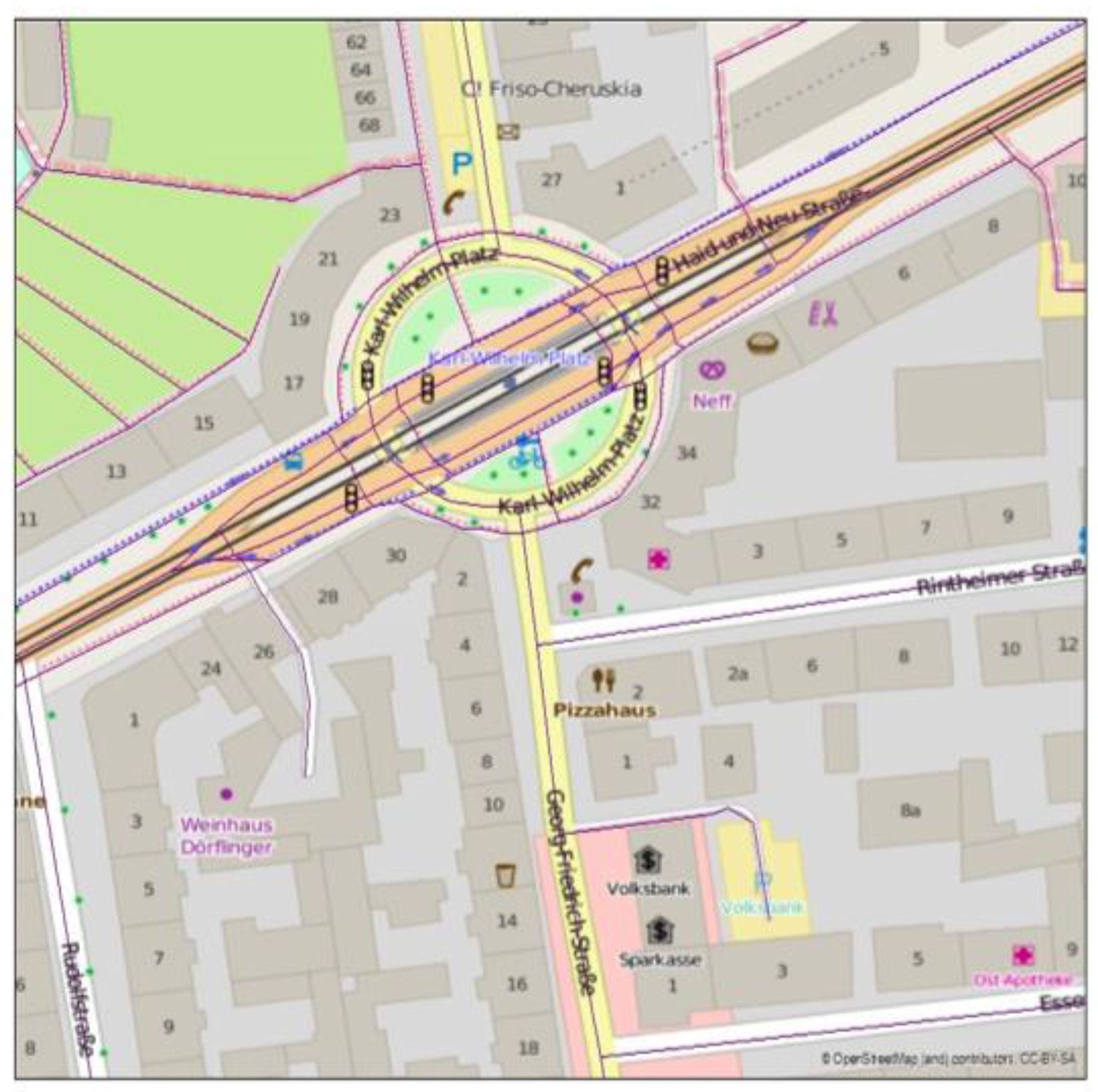
GIS information is also prone to errors; it may have been poorly registered, objects are not located correctly, etc. For instance, OSM has around a five meter registration error in the region of the experiment. Additionally, there are some features that are not properly collected or restored in GIS maps or they are incorrectly labeled. For example, there is a roundabout in the experiment area that is not stored in the GIS map. On-the-fly registration may be performed based on matching static objects from observations and GIS map. However, it is not trivial and we do not use on-the-fly registration here.

The point cloud may be noisy and systematic errors may be introduced to the point cloud as the results of the platform’s motion. The moving least squares (MLS) filter can be used to smooth the surface of objects and suppress the noise. MLS is based on fitting a polynomial surface to the points in the neighborhood [24]. Note that MLS may remove the local changes in the point cloud and could deteriorate the details of the surface. In addition, it may smooth the edges and corners of objects.

5. Experiments

In order to evaluate our algorithms, the KITTI benchmark [25,26] is used. The sensor data includes two monochromic and color image sequences, point cloud collected from the laser scanner, and GPS/IMU integrated navigation solution. During data acquisition, two PointGrey Flea2 gray scale cameras and two PointGrey Flea2 color cameras were mounted in a forward-looking orientation. The Velodyne HD-64E was installed with a rotating axis in the vertical direction. It has a two centimeter range error with 0.09° angular resolution. The OXTS RT 3003 integrated system provides the navigation solution with a two centimeter accuracy in position, and 0.1° in orientation [25,26]. It is mounted in a way that the x and z axes are directed toward the forward and vertical axes, respectively. The sensor configuration is shown in Figure 6.

Figure 6. The sensor configuration on the platform (courtesy of [25,26]).

Figure 6. The sensor configuration on the platform (courtesy of [25,26]).

Dataset #5, collected on 26 September 2011, is used to evaluate the tracking results. In dataset #5 the platform follows a cyclist and a car in an urban area. Buildings, road signs, and parked cars are static objects in the scene. Figure 7 shows images taken at two epochs of dataset #5.

Figure 7. Dataset #5 KITTI; (a) first epoch, (b) after 10 seconds.

Figure 7. Dataset #5 KITTI; (a) first epoch, (b) after 10 seconds.

6. Results

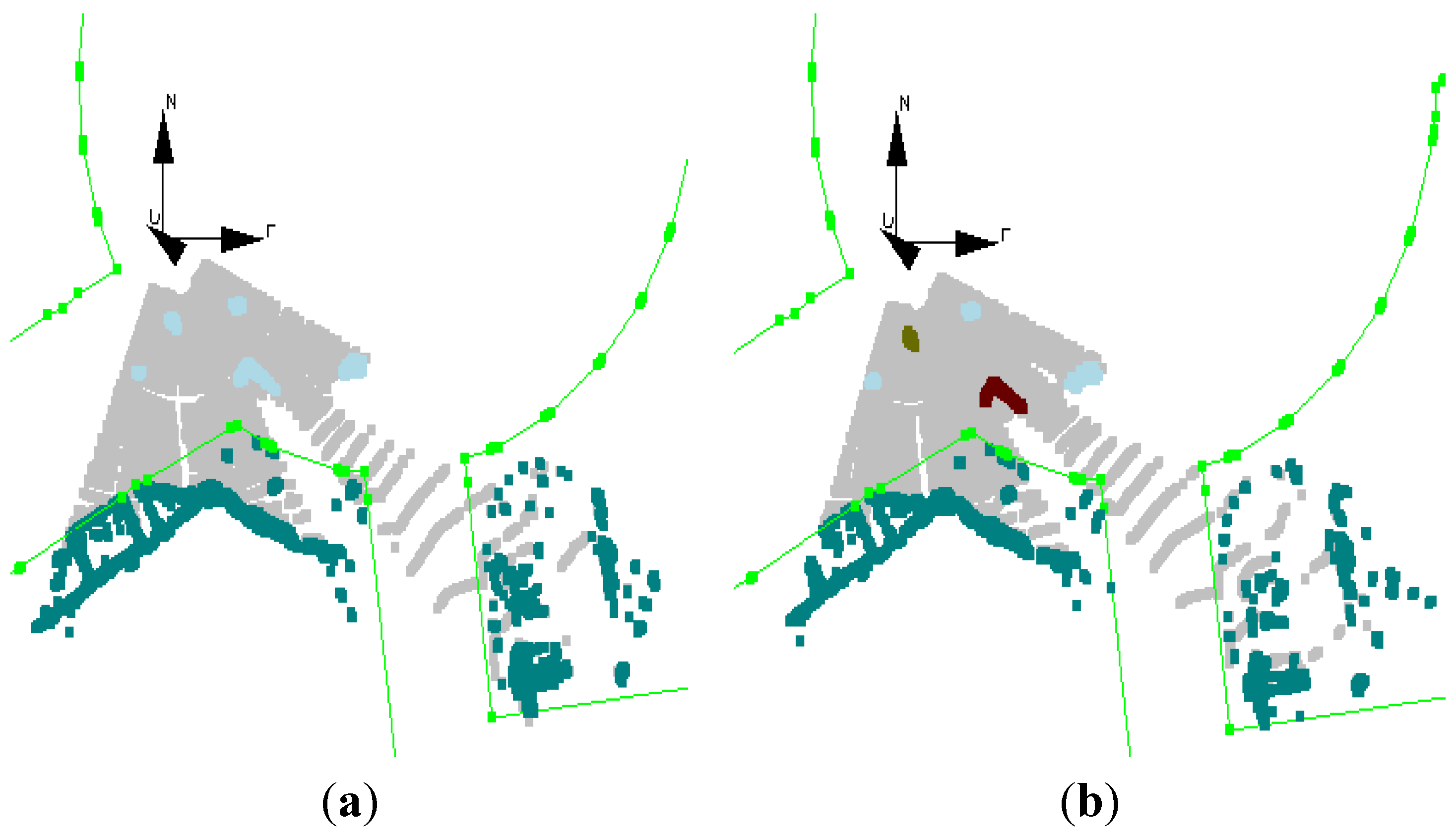
As mentioned before, the segmented objects are assumed to be static at the beginning. Figure 8a shows the static objects of dataset #5, marked light blue, at the first epoch. The moving objects, a cyclist and a car are detected shortly after (0.4 s), shown in Figure 8b. As can be seen in Figure 7a, there is a pedestrian in the scene (at the right side of the image), which is not detected as a moving object. There are two possible reasons: First, the motion of the pedestrian is not significant, and second, the pedestrian shortly goes invisible.

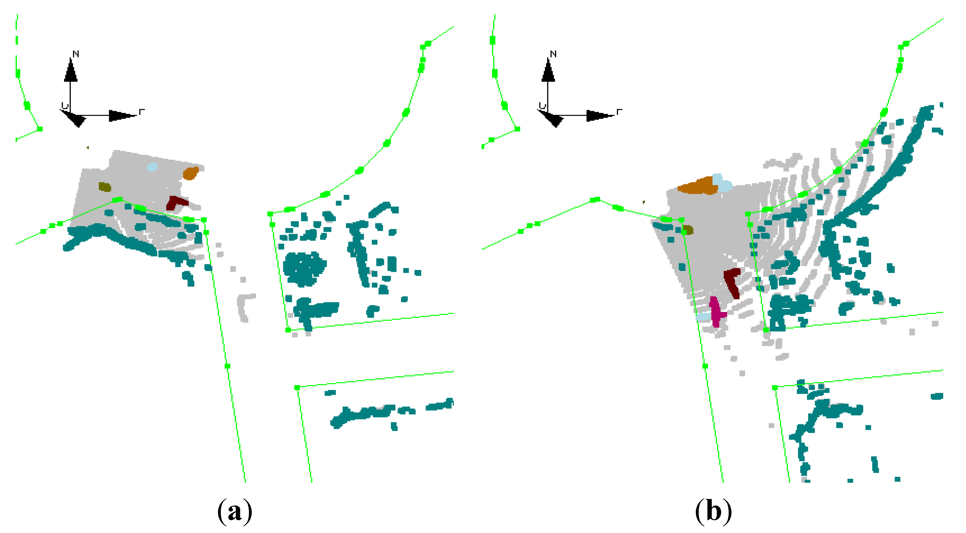
The color, shown in the figures, is randomly assigned to new objects. If an object is tracked, the color in the previous epoch is used for the current epoch. Therefore, if the color of an object remains unchanged the object is successfully tracked. In Figure 9a,b, the moving objects, the cyclist and the car, are tracked correctly and their colors are preserved, but some of static objects are incorrectly labeled as moving objects at a few epochs. Since this fictitious motion of static objects is random, the Kalman filter can filter it out.

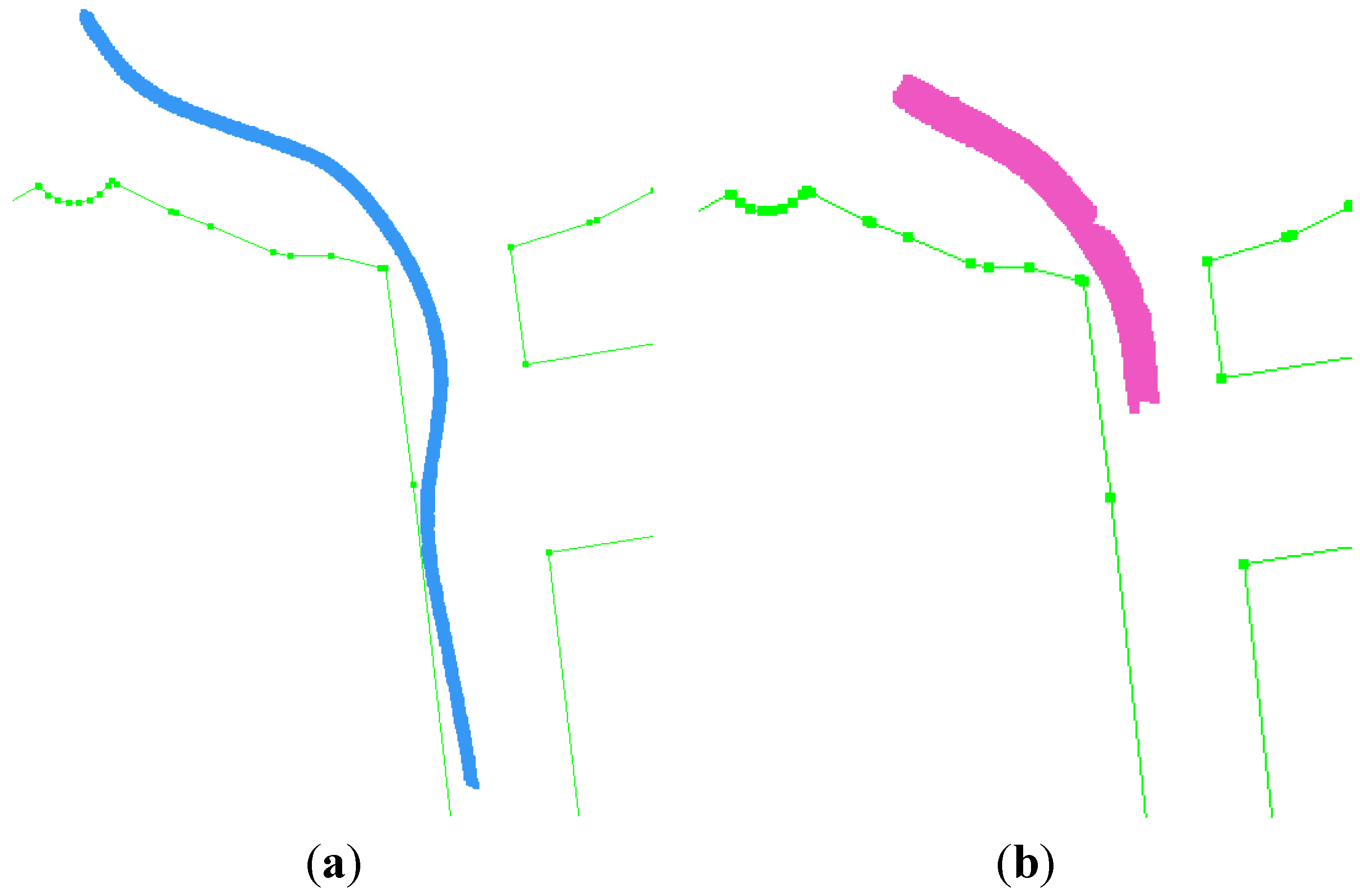
The tracked cyclist and car are shown in Figure 10a,b, respectively. The cyclist is in front of the platform during the experiment. The car is close to platform at the beginning of the experiment, but it speeds up eventually and goes farther. Since our approach focuses on moving objects close to the platform, we stop tracking the car when it goes too far.

The cyclist is closely followed by the platform during the experiment. This experiment has 154 epochs and the cyclist is visible in all epochs. Our tracking algorithm can detect and track the cyclist in 150 epochs. The car is in front of the platform, but it speeds up and it goes far from the platform and, thus, we do not follow it anymore. Therefore, we detect and track the vehicle only in 76 epochs.

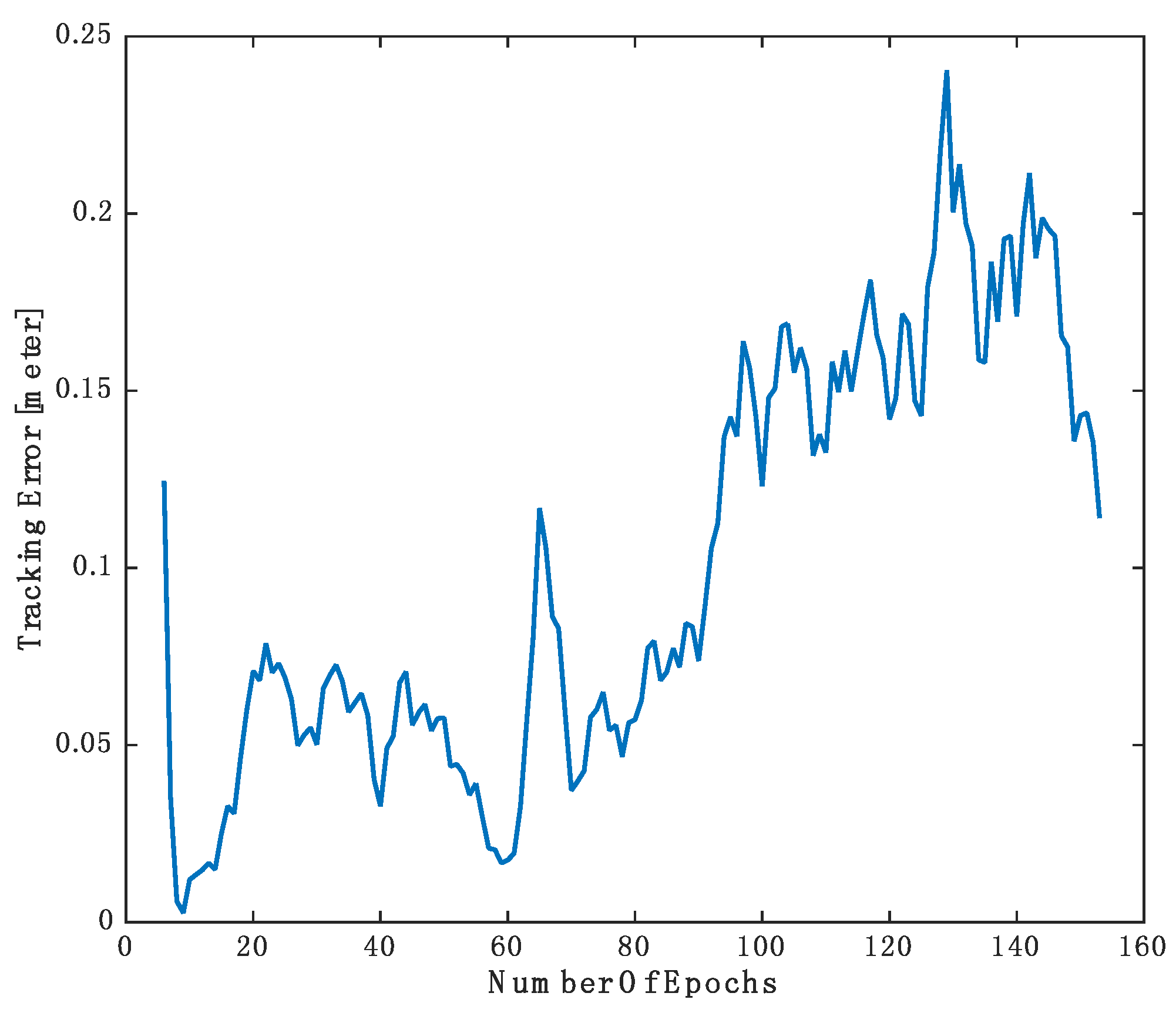
The ground truth position of the cyclist is provided in the KITTI dataset. We compared the tracking results of our approach with the ground truth and the results are shown in Figure 11. The tracking error is the Euclidean distance between the position of the tracked cyclist and the ground truth. Initially, the cyclist is assumed to be static object and the algorithm recognized it as moving object after four epochs. In the first epochs, the Kalman filter is converged and the tracking error drops significantly. After the Kalman filter is stabilized, the tracking error may fluctuate depending on the severity of the occlusion, the navigation solution accuracy, and the motion dynamic of the object. Video of the tracking of moving objects is provided in supplementary materials.

Figure 8. (a) Tracking results at first epoch (dataset #5); all objects labeled as static; (b) the car (brown L shape) and cyclist (green dot) are labeled as moving objects after 0.4 s.

Figure 8. (a) Tracking results at first epoch (dataset #5); all objects labeled as static; (b) the car (brown L shape) and cyclist (green dot) are labeled as moving objects after 0.4 s.

Figure 9. (a,b) Cyclist and car are correctly tracked. However, few static objects are incorrectly labeled as moving objects.

Figure 9. (a,b) Cyclist and car are correctly tracked. However, few static objects are incorrectly labeled as moving objects.

Figure 10. Tracking of (a) a cyclist and (b) a car over time. The car goes too far after a few seconds and it is not an object of interest anymore.

Figure 10. Tracking of (a) a cyclist and (b) a car over time. The car goes too far after a few seconds and it is not an object of interest anymore.

Figure 11. Tracking error of the cyclist.

Figure 11. Tracking error of the cyclist.

7. Conclusions

In this paper, multiple sensors are applied to track the moving objects around a platform in real life scenes, using GPS/IMU navigation solution, images, point cloud, and prior information (GIS maps). The reference frame for moving object tracking is defined based on the GPS/IMU navigation solution and calibrated lever-arms and boresights were used to obtain the imaging sensors’ pose. Prior information is retrieved from OpenStreetMap and used to filter unneeded points from the point clouds. Finally, a bank of Kalman filters is utilized in tracking every object in a scene.

The results show that objects can be tracked and labeled as moving object after a few epochs. Though noisy and cluttered static objects may be labeled as moving objects, they are likely to be filtered out by the Kalman filter after a few epochs. The tests using the KITTI dataset have shown that moving objects can be accurately tracked over time.