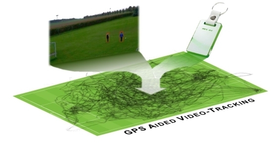
GPS-Aided Video Tracking

Abstract

Tracking moving objects is both challenging and important for a large variety of applications. Different technologies based on the global positioning system (GPS) and video or radio data are used to obtain the trajectories of the observed objects. However, in some use cases, they fail to provide sufficiently accurate, complete and correct data at the same time. In this work we present an approach for fusing GPS- and video-based tracking in order to exploit their individual advantages. In this way we aim to combine the reliability of GPS tracking with the high geometric accuracy of camera detection. For the fusion of the movement data provided by the different devices we use a hidden Markov model (HMM) formulation and the Viterbi algorithm to extract the most probable trajectories. In three experiments, we show that our approach is able to deal with challenging situations like occlusions or objects which are temporarily outside the monitored area. The results show the desired increase in terms of accuracy, completeness and correctness.

1. Introduction

In many research fields and applications, tracking moving objects plays an important role. This is especially true in situations where the objects’ positions and movements are analyzed to evaluate or to gain knowledge about their behavior. Typical application scenarios are the observation of persons moving through a city, a place or a building, or animals in their environment. Global navigation satellite system (GNSS) receivers as well as video- or radio-based tracking systems are technologies typically used for this purpose. Those observations can last for long time periods, often for several months, and therefore provide large datasets reflecting the movements of the objects. Often, the analysis is required in real time and the effort to analyze the resulting data is so extensive that it cannot be done manually; therefore, automatic approaches are necessary to analyze and interpret the trajectories.

An important application is the use of tracking systems in the sports domain, e.g., the goal line technologies in soccer or the “Hawk-Eye” [1] in tennis, which is able to determine the ball’s ground touching point and is consulted by a player or referee in unclear situations. In these applications object positions in the range of a few centimeters are required for each point in time. In other words: If during the observation, decisions have to be made which require centimeter-scale accuracy, neither missing data nor data with lower accuracy are acceptable. Further examples are the offside decision in soccer or any other decision that deals with the question of whether the ball has crossed a line or not. Besides the position of the ball, the exact position of all players is increasingly important for the tactical analysis of game situations.

Neither global positioning system (GPS) nor video tracking, which are the most prevalent technologies, are not suitable as standalone solutions, which is described in related studies. There are several investigations on the validity and reliability of GPS measurements in sports [2,3,4,5,6]. Most of them evaluate different devices based on their accuracy and compare the measured performance values to ground truth data. They conclude that the devices provide acceptable relative accuracies, e.g., in terms of the covered distance. However, if a high absolute accuracy is required, the usual non-differential GPS accuracy of only 3 meters at best is not sufficient. On the contrary, in video-based tracking the geometric accuracy is high, ranging between about 0.5 to a few centimeters [1]. An extensive review of vision-based motion analysis is given by Barris and Button [7]. They focus on the sports domain and discuss the limitations and the reliability of different tracking systems. Often, the video-tracks are evaluated manually or semi-automatically. When it comes to automated systems, Barris and Button point out problems of tracking objects in dynamic and crowded environments, leading to incomplete trajectories.

In summary, GPS tracking generally lacks the required absolute accuracy, and video-based tracking often suffers from a lower completeness induced by detection and tracking issues mainly caused by object occlusions.

Different approaches exist to tackle this problem. Most often, multiple cameras are used to get different perspectives on the objects [1,8,9,10]. However, such solutions require suitable installation locations for the cameras, a corresponding setup effort, and are usually expensive. For instance, professionally used camera tracking systems require from 6 to 8 high-end cameras. Other related work either focuses on using histograms of color components of RGB or HSV of the object detections [11], motion patterns [12] or rectangle features in addition to edge orientation histograms [13] to track and distinguish between multiple objects.

Approaching this problem by using differential GPS receivers which are able to localize with a very high accuracy (down to 1 cm) leads to the requirement that each of the observed objects has to be equipped with such a device. This is not practical, especially in the domain of sports.

Our approach is to combine both technologies and thereby to exploit their relative strengths and reduce their weaknesses. That is, GPS tracking provides continuous trajectories of single objects, which, however, are typically of low positional accuracy. Cameras, on the other hand, provide a higher geometric accuracy but are prone to object occlusions, which result in interrupted or incomplete trajectories. In our case, we improve the GPS trajectories using the high accurate positions received from the video tracking. In order to do so, we have to fuse data from both sources. This type of problem can be readily modeled as a dynamic Bayes network, where the state progresses in discrete time steps, the observations are the position measurements, and the unknown assignments between GPS and video observations are hidden states to be estimated. Since this form of a hidden Markov model (HMM) [14] is a linear network without cycles, it allows for an exact and efficient solution of the most likely object assignments using the well-known Viterbi algorithm [15]. Its suitability has also been shown in similar applications [16,17]. An advantage of using this algorithm in our approach is that if our tracking fails because of occluded or missing objects, it will be able to “recover” the objects after the situation has cleared up and trace back their most likely path, in contrast to purely video-based methods.

The remainder of this article is structured as follows. In the next section, the approach, including data acquisition and processing methods, is described in detail. Afterwards, an experiment is presented, followed by the presentation and discussion of the results. The article is closed by a conclusion and outlook.

2. Data Acquisition and Processing Methods

2.1. The Approach

Given a soccer scenario, the setup for the tracking task is as follows: We have one camera to observe the entire scene. Next, we equip each observed person with a GPS unit. Depending on the hardware used, our approach can be designed in a centralized or in a decentralized way [18]. The latter requires sensors which are able to perform computations as well as to communicate their aggregated results. Alternatively, if the sensors are not able to communicate, the recorded data can be transferred and processed afterwards. Since our GPS devices are only able to log data, we process all data (from GPS and camera) at a central processor. As shown in Figure 1, the sensors provide the data in the form of tracking points (tp, id of GPS unit) and camera detections (d_i, camera), which are information tuples containing at least the object position and the timestamp. The latter is necessary in cases where there is no temporal synchronization between camera and GPS devices.

The sections below describe the consecutive processes according to the scheme in Figure 1, from the input data to the final trajectories.

Figure 1. Overall structure of our approach.

Figure 1. Overall structure of our approach.

2.2. Input Data from Sensors

GPS data: Depending on their specification, the used GPS devices provide 3D position data with a rate of 1 to 10 Hz. In cases of quite fast movements with frequent turns, as occur in the sports domain, temporal resolutions with a 1 Hz update rate or lower can be too low to capture the movements in full detail [2,3]. In order to enable a reasonable use of the data for our approach, a rate of at least 5 Hz is required. A tracking point (tp), from one of the devices at one time step has the form tp_i = (position, timestamp, objected)_i.

Camera data: In our experiments, we update the state using GPS and camera data simultaneously. Therefore, we only need to receive position data from the camera at the same rate as the GPS sampling rate. The object positions are determined from the video stream using image processing algorithms, which are applied to the successive frames recorded by the camera. For this purpose several approaches exist to detect objects in images. In [19] an overview is given. Since we use a static camera setting without any camera movement or zoom, we are able to use a background subtraction algorithm [20] to detect changes (see Figure 2b) in front of a continuously learned background (see Figure 2a). The results are filtered using morphologic operations, as well as geometric and spatial constraints to eliminate most of the false signals. Subsequently, the changes are processed to lead to so-called potential objects in each time frame, mainly bounding boxes with additional information, which we call “detections” in the remainder of this paper.

A hypothesized object (here a person) is represented by a bounding box. The object position is determined by the bottom center of the bounding box (Figure 2c). In contrast to the GPS tracking points, which contain unique object IDs, camera detections are not assigned to objects. For the fusion process at a later stage, we add a feature vector to our observations, which is computed for each detected region in the camera image. We used a histogram, which captures the distribution of hue values inside the detection’s shape. Thus, the information received from the camera at one time step is the detections D = {d₁, d₂, …, d_m} with d_i = (position, timestamp, histogram)_i. This presupposes that detections represent individual objects, which, however, can be violated, when people are close to each other.

Figure 2. (a) The background image of the observed scene. (b) The detected changes. (c) The resulting object detections framed by red bounding boxes.

Figure 2. (a) The background image of the observed scene. (b) The detected changes. (c) The resulting object detections framed by red bounding boxes.

2.3. Preprocessing the Data

Due to the fact that we intend to merge the data of different data sources with different coordinate systems (GPS data and camera data), we have to temporally and “spatially” synchronize them. To this end we transform both into a common local coordinate system a using a precomputed homography for the camera data. The temporal synchronization is done with the help of the timestamps. The merged data is the input for the fusing method (see Figure 1).

2.4. Data Fusion

The fusion of the incoming tracking points of the camera with GPS trajectories is based on a HMM and the Viterbi algorithm, which determines the most likely trajectories of the observed objects. As schematically illustrated in Figure 3, the challenge is to identify corresponding data points between camera detections on the one hand and GPS trajectories on the other hand.

Figure 3. The data assignment task: The initial setting contains two continuous GPS trajectories (connected red and yellow dots) and unassigned camera detections (isolated blue boxes), both in the common local coordinate system. The time progression is indicated below.

Figure 3. The data assignment task: The initial setting contains two continuous GPS trajectories (connected red and yellow dots) and unassigned camera detections (isolated blue boxes), both in the common local coordinate system. The time progression is indicated below.

2.4.1. Hidden Markov Models

Since there are several descriptions and tutorials on HMMs [14,21,22], we only introduce them briefly and focus on our adaptations. HMMs are defined to be a quintuple of $\text{λ}=\left(S;V;A;B;\text{π}\right)$, where $S=\left\{S_{1 },S_{2 },\dots , S_{m },\right\}$ are the states and $V=\left\{V_{1 },V_{2 },\dots , V_{n },\right\}$ the observations. Furthermore,

A = {a_ij}, a_ij = P(S_j (t + 1)|S_i (t))

(1)

are the state transition probabilities, where t is the time step,

B = {b_jk}, b_jk = P(V_k (t)|S_j (t))

(2)

are the measurement probabilities under the condition the real state being S_j and

$$\text{π}=\left\{{\text{π}}_i\right\} {\text{π}}_i=P\left(S_i\left(t=0\right)\right)$$

(3)

are the initial state probabilities.

In our case, we intend to improve the objects’ GPS positions using more accurate positions obtained through video tracking. Therefore, representation in the form of a HMM is as follows. The current (hidden) state S includes the estimated position, the assignment to a detected region in the camera image, and the hue histogram. The observations V are given by the positions measured by the camera and GPS sensor. We have made a number of modifications to this model. First, since the standard deviations of the camera position measurements are much smaller than those of the GPS measurements, the best position estimate will be almost independent from the GPS position. Also, we have so far not included a kinematic model (e.g., acceleration, velocity, heading parameters) into the state and state transitions. Those two modifications lead to a simplified representation where the position component of the state is set to the camera position measurement derived from the assigned image region. Thus, given a state, the measurement probability B is only dependent on the distance between the state’s position component and the GPS position, which is in turn the distance between the camera and GPS position measurement.

The state transition probabilities B are calculated by comparing the feature vectors of successive states. In our case, we use histogram similarities and movement model restrictions. As histogram similarity measure we use the histogram intersection, which provides values in the range between 0 (no similarity) and 1 (equal) and is defined as

$$p\left(H_1, H_2\right)= {\displaystyle \sum }_I\min \left[H_1 \left(I\right), H_2 \left(I\right)\right]$$

(4)

where I indexes all hue values. Again, we simplify the model in that we do not filter the hue histogram in the current state. Thus, after an image region is assigned, the hue histogram in the state is replaced (and not updated) by the hue histogram obtained from the image region.

A second component of the transition probabilities is an indicator function, which is 1 if the subsequent position is within reach of the previous position. That is, we require the velocity v of the objects to be lower or equal to a maximum velocity

v ≤ v_max

(5)

where v_max is chosen depending on the scenario.

Another substantial modification concerns the simultaneous computation of multiple tracks. So far, we have described the HMM for a state consisting of a single position, assignment and hue histogram. However, we are interested in assigning multiple trajectories simultaneously, since one of the main purposes is to uncover the correct assignments for multiple trajectories, especially if they are close to each other. That is, we are interested in unique assignments of GPS positions to image regions. Similar to [23] we define our states to contain tuples of assignments instead of single assignments. These tuples are the variations of the current set of detections. As an example, given the set of l = 3 detections {F, G, H} as it occurs in time step 2 (Figure 3) and the observation of k = 2 objects, there are $m= \frac{l!}{\left(l-k\right)!}=6$ possible assignments without repetitions, namely {(F,G), (F,H), (G,F), (G,H), (H,F), (H,G)}. Thus, any state sequence will define a sequence of assignment tuples.

Further, we have to handle the problem of undetected objects that are either occluded or have left the field of view. For this purpose, we add dummy assignments, which represent the state of “not detected”. Since these “virtual detections” represent missing measurements, their effect is that the previous position and hue histogram (in the state) are left unmodified. In the previous example, the set of detections changes to {F, G, H, Ø} with Ø being the dummy detection. The assignment set increases to m = 12 + 1 = 13 elements. Note that there is an additional assignment (Ø, Ø) for the case that both objects are not detected. In Figure 4 the HMM is illustrated for the example given in Figure 3.

Figure 4. The HMM for multiple trajectories. On top, the dynamic Bayes network formed by the sequence of states (in white). The colored nodes below are the possible state values (the assignment tuples) for the state sequence S1 to S6. The colors encode the number of dummy assignments (green: only real; yellow: at least one dummy; red: only dummy assignments). The gray edges symbolize the transition possibilities between the corresponding states (shown for the transitions between t₀ and t₁).

Figure 4. The HMM for multiple trajectories. On top, the dynamic Bayes network formed by the sequence of states (in white). The colored nodes below are the possible state values (the assignment tuples) for the state sequence S1 to S6. The colors encode the number of dummy assignments (green: only real; yellow: at least one dummy; red: only dummy assignments). The gray edges symbolize the transition possibilities between the corresponding states (shown for the transitions between t₀ and t₁).

The initial states of our model are initialized with uniformly distributed probabilities:

$${\text{π}}_i= \frac{1}{m}$$

(6)

Effectively, this means that we use an uninformative prior, i.e., the most probable trajectories do not depend on an initial state.

Since the state now contains assignment tuples, we have to modify the state transition and measurement probabilities accordingly. As for the state transition, we treat the histogram similarities as probabilities of independent random variables so that their joint probability is given by the product of their marginal probabilities. Thus, if the tuples S₁ and S₂ are given with K being the number of objects and H_1,i and H_2,i being the ith histogram of the first and second tuple, respectively,

$$p\left(S_{1 }, S_{2 }\right)= {\displaystyle \prod }_{i=1, \dots , K}p\left(H_{1,i }, H_{2,i }\right)= {\displaystyle \prod }_{i=1, \dots , K}{\displaystyle \sum }_I\min \left[H_{1,i} \left(I\right), H_{2,i} \left(I\right)\right]$$

(7)

is the overall similarity, and since we impose in addition a maximum velocity constraint, we obtain the following state transition probabilities:

$$a_{ij}= \{\begin{array}{c}p\left(S_{i }, S_{j }\right),v \le v_{max} \\ 0, otherwise\end{array}$$

(8)

As for the measurements, we assume the GPS observations to be independent and identically normal distributed. Therefore, we model their probabilities according to the product of their densities, which is

$$b_{jk}= {\displaystyle \prod }_i\frac{1}{\sqrt{2\text{π}} {\sigma }_{GPS}}{e}^{-\frac{1}{2}\bullet \frac{d_i^2}{{\sigma }_{GPS}^2}}= {\frac{1}{\sqrt{2\text{π}} {\sigma }_{GPS}}}^K{e}^{-\frac{1}{2}{\Sigma }_i\frac{d_i^2}{{\sigma }_{GPS}^2}}$$

(9)

where d_i are the pairwise Euclidean distances between the positions in the state S and the positions from the assigned (GPS) observations V. The GPS inaccuracy is modeled using the standard deviation σ_GPS.

2.4.2. The Viterbi Algorithm

We tackle the problem of determining the most likely state sequence $S_{V }=\left(S_{1 },\dots , S_{T }\right)\in S$, given the sequence of observations $O=\left(o_{1 },\dots , o_{T }\right)\in V$ by applying the Viterbi algorithm [15]. It works recursively and is efficiently implemented using dynamic programming. The algorithm can be summarized by the following steps. While $S_{V_t}^{*}$ holds the most probable predecessor of the state at time step t, P_t is the probability of the most probable state sequence.

Initialization

$$P_{t=0} (S_i)={\text{π}}_i\bullet b_{0,i}, 1 \le i \le m$$

(10)

Recursion

$$P_t(S_i)=b_{t,i}\cdot \underset{1\le j\le m}{\text{max}}\left(a_{ji}\cdot P_{t-1}(S_j)\right) 1\le i\le m,1\le t\le T$$

(11)

$$S_{V,t}^{*}(S_i)=\underset{1\le j\le m}{argmax}\left(a_{ji}\cdot P_{t-1}(S_j)\right) 1\le i\le m,1\le t\le T$$

(12)

Backtracking

$$S_{V,t}=S_{V,t+1}^{*}(S_{V,t+1})$$

(13)

In Figure 5 the process and the most likely path (also termed the Viterbi path) for the example given in Figure 3 are visualized. The blue encircled nodes form the Viterbi path, which represents the sequence of assignments and positions for both object trajectories.

2.5. Output Trajectories

Having calculated the Viterbi path, we can generate the trajectories for each object. For this purpose we follow the path and simply output the positions in the state (which, in our case, correspond to the positions of the assigned image detections), together with their timestamps (see Figure 6).

Figure 5. The resulting Viterbi path (blue) for the given example.

Figure 5. The resulting Viterbi path (blue) for the given example.

Figure 6. The trajectories (red, orange) are generated from the assignment tuples contained in the nodes of the Viterbi path. Some detections have been discarded (isolated gray boxes).

Figure 6. The trajectories (red, orange) are generated from the assignment tuples contained in the nodes of the Viterbi path. Some detections have been discarded (isolated gray boxes).

2.6. Performance of the Algorithm

The performance of our algorithm depends on the number of observed objects and camera detections in each time step, which determine the number of possible states m. Then the complexity of the Viterbi algorithm is O(m²t), where t is the number of time steps. Therefore, it is important to use an efficient object detection algorithm, which minimizes the number of false detections.

3. Experimental Section

3.1. Experiments

Since we intend to create a tracking solution which provides accurate, complete and correct object trajectories, we have designed three experiments. In these experiments, data is generated which we use to analyze the performance of our algorithm. In the first experiment we analyze the localization accuracy of GPS tracking and camera-based tracking. In the second experiment we focus on the tracking quality, especially the completeness and correctness of the resulting trajectories. Through that experiment, we wanted to prove that our approach is able to handle situations in which objects are out of sight for some time. In the last experiment we wanted to demonstrate the ability to track multiple objects, even though they are very similar and sometimes occluded.

In all experiments we try to compare the results of our approach with those of a video-only version of our approach and the GPS traces. In order to obtain the results of a purely video-based method we ran our algorithm a second time without using the GPS information. The assignment is then exclusively based on the color histograms of the objects and the movement model restrictions.

3.2. Experimental Setup

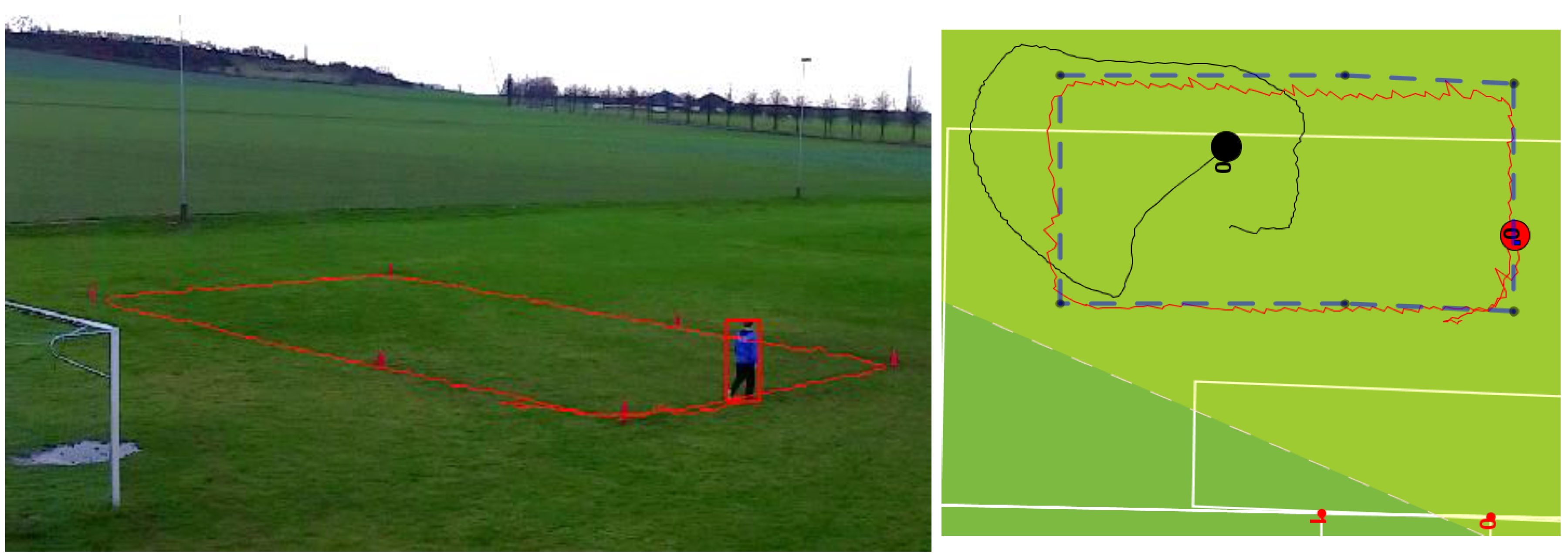
3.2.1. Experiment 1—Accuracy

In the first experiment we equipped the observed persons with GPS loggers which support 5 Hz logging. The manufacturer specifies their position accuracy with 3.0 m 2D-RMS without aid. A smartphone camera with a full-HD resolution (1920 × 1080 px) with disabled auto-focusing functionality was used. It was placed in a higher location to get a better viewing angle on the scene. The sketch-map in Figure 7 shows the setting in a top view.

For the determination of accuracy, a person moves several laps on a predefined rectangular track (see Figure 7). Further, the person is instructed to move with an increased velocity for each lap, walk, run and sprint. As ground truth data, we assume linear connections between the four corner points, for which the coordinates are known.

Figure 7. Overview of the setup for the first and second experiment: The four edge points waypoints for the first experiment are marked in red. The gray traces are the locations of the detections of the camera.

Figure 7. Overview of the setup for the first and second experiment: The four edge points waypoints for the first experiment are marked in red. The gray traces are the locations of the detections of the camera.

3.2.2. Experiment 2—Completeness and Correctness

In the second experiment we use the same technical and installation settings as in the previous experiment. We observe two persons for about 4 min (5 Hz sampling rate of camera and GPS units), who move randomly through the scene, cause occlusions by moving close to each other and even leave the field of view. This time, the ground truth data is generated by a manual assignment of the camera detection to the persons. We do not have any ground truth trajectories as a reference to compare to, because this experiment is meant to evaluate the assignments. Since we are using the same technical equipment and installation, we assume the accuracy to be the same as in the first experiment. However, with the help of the available ground truth data we can evaluate the correctness of the assignments, which is actually the purpose of this experiment. We used the following parameter settings: σ_GPS = 12 m, v_max = 8m/s.

3.2.3. Experiment 3—Multiple Object Tracking

The last experiment consists of tracking 4 out of 16 players during a soccer game. For this experiment we use a soccer dataset published by the Fraunhofer ISS in connection to a data challenge of the ACM DEBS 2013 [24]. It contains a video (1920 × 1080 px) as well as the trajectories of 16 players, a referee and the used balls. The trajectories have been recorded by their own radio-based tracking system with a high accuracy of few centimeters. Since this is slightly better than we expect from ours, we use them as reference trajectories. As no GPS information is contained in this dataset, we have generated it by adding noise to the highly accurate reference trajectories. To mimic the inaccuracies of GPS, we used a systematic shift of the whole trajectory in a random direction and normal distributed noise with a standard deviation of 5 meters. Further, it should be noted that the players of each team have similar clothes. For that reason the detections will also have similar color histograms. This is important, because our approach makes use of the histograms to distinguish between objects. In this experiment we therefore want to show that our approach is able to deal with similarly colored multiple objects. The parameter setting is: σ_GPS = 12 m, v_max = 8m/s.

4. Results

4.1. Experiment 1—Accuracy

In Figure 8, the results of the first experiment are visualized. As expected, the camera is significantly more accurate than the standalone GPS measurement. The camera trajectory’s error mainly depends on the object detection algorithm used. In our case the background subtraction algorithm provides detections with a standard deviation of about 0.25 m to the ground truth track. Please note that this error is also caused by the tracked person, who does not move exactly on the defined track. We evaluated the GPS trajectory using the trajectory obtained from the camera observations as ground truth and obtained a standard deviation of approximately 10 m. We do not compare the purely video-based methods to our combined approach in terms of accuracy, since both use the same camera detections and thus yield the same accuracy.

Figure 8. The resulting trajectories of the accuracy experiment: GPS (black) and result of our approach (red). The dots are the object current position determined by GPS (black) and our approach (red). The ground truth polygon is marked by a dashed blue line.

Figure 8. The resulting trajectories of the accuracy experiment: GPS (black) and result of our approach (red). The dots are the object current position determined by GPS (black) and our approach (red). The ground truth polygon is marked by a dashed blue line.

There are at least two further issues that influence the exact localization of persons with our current approach. First, it strongly depends on how the position is detected. For instance, we represent the detection as a bounding box, and use the bottom center of this box to define the person’s position, assuming that this is a sufficiently accurate representation of the (fictitious) body center projected to the ground. However, if a person stretches out an arm or leg, this point will not be a correct representation of this body center anymore. Second, the localization error is related to the object’s distance to the camera. Due to the image perspective, the error is not homogeneous in the observed area, but rather increases with increasing distance. In Figure 9b (region C), this effect can be clearly observed in the lower left part of the soccer field where the trajectories appear to be strongly jagged.

4.2. Experiment 2—Correctness of Assignments

The results of our second experiment with two persons are shown in Figure 9a,b. Due to the fact that the GPS tracking cannot lead to false assignments, we only compare our combined solution to the generated ground truth data. In order to do so, we calculated the number of correct and false assignments, as shown in Table 1. We obtained a recall ratio of 94.2% and 5.8% misses, for a total number of 2238 detections. Please note that detections containing merged image regions of both persons, caused by partial occlusion, have been marked as erroneous in the ground truth data, because we were unable to label them unambiguously. Thus, we will expect an even better recall ratio and lower number of false detections if we improve our handling of merged blobs. Also, errors in the detections are still included, such as false detections caused by moving objects in the background. Thus the error rate of about 10% can still be decreased by adjusting the detection algorithm, e.g., by specifiying a region of interest. In Figure 9c the trajectories are shown which result when using no GPS information. In this setting, in which the persons are not similarly clothed, the trajectories look fine, too, except for some incorrect assignments, which can be identified as jumps in the traces (long straight lines). The performance values are accordingly lower.

Table 1. Performance of our tracking algorithm.

	With GPS	Without GPS
Total (objects/unassignable)	2238 (2030/208)	2238 (2030/208)
Recall (%)	2109 (94.2%)	2013 (89.9%)
Misses (%)	129 (5.8%)	225 (10.1%)

Table 1. Performance of our tracking algorithm.

	With GPS	Without GPS
Total (objects/unassignable)	2238 (2030/208)	2238 (2030/208)
Recall (%)	2109 (94.2%)	2013 (89.9%)
Misses (%)	129 (5.8%)	225 (10.1%)

Moreover, we had a closer look at situations which seem to be an issue in many video-based tracking solutions. This approach is also able to handle situations where an object leaves and reenters the scene. For instance, in region A of Figure 9b, the red-colored trajectory leaves the right border of the image and appears again at a later point in time (see Figure 10). Furthermore, there are several frames in which a person is occluded by another person or by an obstacle like the flagpole on the left. For example, we show one of those in region B of Figure 9b and in Figure 11, respectively. In those cases, the algorithm succeeds in keeping the correct assignment until the situation clears up.

Figure 9. The results of the second experiment: (a) the scene containing both tracked objects and their trajectories; (b) top view of the complete dataset including the trajectories generated by GPS (both in black) and by our approach (red, green). Furthermore, three regions A, B and C (blue) are marked which contain situations being referred to in the text. (c) The result when GPS information is not used.

Figure 9. The results of the second experiment: (a) the scene containing both tracked objects and their trajectories; (b) top view of the complete dataset including the trajectories generated by GPS (both in black) and by our approach (red, green). Furthermore, three regions A, B and C (blue) are marked which contain situations being referred to in the text. (c) The result when GPS information is not used.

Figure 10. Situation in which a person leaves the field of view for about 8 s. The algorithm manages to keep the correct assignment (sequence from top left to bottom right).

Figure 10. Situation in which a person leaves the field of view for about 8 s. The algorithm manages to keep the correct assignment (sequence from top left to bottom right).

Figure 11. Another situation where the person marked green is occluded for about 1.5 s (8 frames). The assignment is continued correctly after the situation has cleared up.

Figure 11. Another situation where the person marked green is occluded for about 1.5 s (8 frames). The assignment is continued correctly after the situation has cleared up.

In the case that an assignment fails, the Viterbi algorithm has the ability to change the assignments retroactively, in contrast to other tracking algorithms that are only able to decide for the current time step. This is due to the fact that the Viterbi algorithm uses all observations to compute the most likely path, whereas sequential tracking algorithms compute the most likely (current) state, given all previous observations. In Figure 12 an example for such a retroactive assignment correction is shown. While in Figure 12a the last parts of the trajectories are interchanged (the correct assignment would be the blue dressed person to the red trajectory), the assignments have been corrected in Figure 12b, a few time steps later. Of course, these assignment corrections would not be suitable if real-time movement analysis is required (unless a time lag would be tolerable).

4.3. Experiment 3—Multiple Object Tracking

In Figure 13 and Figure 14 the results of our third experiment are given. The experiment shows that our approach is able to track multiple objects which are often occluded and similarly clothed. When comparing the resulting trajectories to their reference traces (black) in Figure 14 (left) we observe a lower accuracy (which is mainly a problem of the object detection algorithm) but we also notice a correct player assignment. This can be recognized by the very similar shape of the corresponding trajectories. However, sometimes players are not tracked correctly, but are successfully recovered when the situation has cleared up. As shown in the example, the green player is merged with another player in Figure 13 (1) and totally lost in (2) (symbolized by a gray colored bounding box), has been recovered in (3) and successfully tracked until (4). The situation is similar when looking at the red player who is confused with another player in (3) and recovered in (4). This basically can be traced back to the incorporation of GPS information. If we do not use the GPS locations, the result looks like in Figure 14 (right). This is not surprising, as the identically dressed players cannot be distinguished based on color histograms. In this case adding and/or replacing features (like those proposed in [11] or [12]) would improve the distinguishability of the objects.

Figure 12. An example for the “retroactive” assignment correction: (a) the last trajectory parts (yellow box) are assigned wrongly; (b) the assignment has been corrected a few time steps later.

Figure 12. An example for the “retroactive” assignment correction: (a) the last trajectory parts (yellow box) are assigned wrongly; (b) the assignment has been corrected a few time steps later.

The performance values determined in the previous experiments and the described ability to handle difficult tracking issues show that we basically achieved our goal to obtain camera measurement accuracy combined with GPS labeling reliability.

Figure 13. The resulting trajectories of our approach showing the ability to deal with occlusions.

Figure 13. The resulting trajectories of our approach showing the ability to deal with occlusions.

Figure 14. The generated colored trajectories of the tracked players are close to their reference traces (black) (left). The colored dots represent the current player positions determined by our approach. The gray ones are the reference positions. The trajectories obtained from the video-only version of our approach (right). Significantly, the red and the green players are often mixed up with other players.

Figure 14. The generated colored trajectories of the tracked players are close to their reference traces (black) (left). The colored dots represent the current player positions determined by our approach. The gray ones are the reference positions. The trajectories obtained from the video-only version of our approach (right). Significantly, the red and the green players are often mixed up with other players.

5. Conclusions and Outlook

In this work we have presented a method to track objects by integrating two different tracking technologies. Using an HMM model and the Viterbi algorithm, we were able to fuse the data of the different devices and to calculate the objects’ trajectories. The evaluation results show that our approach is able to combine the correct assignment of GPS tracking with the geometric accuracy of video-based tracking.

The general requirements of the presented approach are as follows: First of all, the observed objects have to be equipped with GPS sensors which have to provide their location data. In addition, the objects also have to be detectable by the camera, i.e., they need to be inside the field of view of the camera most of the time. For our experiments, we used a low-cost system which consists of a smartphone and low-cost GPS receivers. The GPS positions were recorded and the trajectory fusion was computed in post-processing on a PC.

If the GPS sensors are able to transmit the current location to a data processor in real-time (this can be the camera itself if it is a smart camera), an online object tracking is be possible, i.e., a real-time solution. This is due to the algorithmic complexity of O (m²) for each frame where m is the number of possible states, which is mainly determined by the number of detections. Although we have shown that the approach works well, there are several open issues for future work. First, the presented approach can be refined and extended. For instance, we could integrate a kinematic movement model for the objects, as well as a more rigorous modeling of the observations, basically leading to a full-fledged Kalman filter step for the continuous state variables. This would ease the integration of other types of observations, at different measurement frequencies, e.g., GPS and radio tracking, camera and radio tracking or multiple camera tracking. Regarding our image processing approach, there are several possible improvements. The image detection could be made more robust if prior information about the expected position were available, such as the position predicted by a kinematic movement model. The computed feature similarities, so far the similarities of the hue histograms, could be extended by image correlation or tracking approaches, which are expected to work better if the persons wear similarly colored clothing. Also, the features derived from the image observations should be part of the state so that they are updated instead of replaced in every time step.

Furthermore, the approach can be transferred to other use cases outside the sports domain. One example is the surveillance of traffic scenarios, like observation of crossing areas or crowded places which can be used by pedestrians as well as other road users. This certainly can also be done by standalone GPS or camera tracking, but in cases where either a higher accuracy, e.g., for movement prediction and collision detection, or a higher reliability, e.g., object tracking in crowded scenes, is required, this approach can be useful. For instance, shared location data of smartphones or car GPS data provided by navigation systems can be combined with video sequences from existing traffic cameras to obtain highly accurate car trajectories.

References

1. Home: Hawk-Eye. Available online: http://www.hawkeyeinnovations.co.uk/?page_id=1011 (accessed on 9 January 2015).
2. Coutts, A.J.; Duffield, R. Validity and reliability of GPS devices for measuring movement demands of team sports. J. Sci. Med. Sport 2010, 13, 133–135. [Google Scholar] [CrossRef] [PubMed]
3. Gray, A.J.; Jenkins, D.; Andrews, M.H.; Taaffe, D.R.; Glover, M.L. Validity and reliability of GPS for measuring distance travelled in field-based team sports. J. Sports Sci. 2010, 28, 1319–1325. [Google Scholar] [CrossRef] [PubMed]
4. Johnston, R.J.; Watsford, M.L.; Kelly, S.J.; Pine, M.J.; Spurrs, R.W. The Validity and reliability of 10 Hz and 15 Hz GPS units for assessing athlete movement demands. J. Strength Cond. Res. 2013. [CrossRef] [PubMed]
5. Randers, M.B.; Mujika, I.; Hewitt, A.; Santisteban, J.; Bischoff, R.; Solano, R.; Zubillaga, A.; Peltola, E.; Krustrup, P.; Mohr, M. Application of four different football match analysis systems: A comparative study. J. Sports Sci. 2010, 28, 171–182. [Google Scholar] [CrossRef] [PubMed]
6. Varley, M.C.; Fairweather, I.H.; Aughey, R.J. Validity and reliability of GPS for measuring instantaneous velocity during acceleration, deceleration, and constant motion. J. Sports Sci. 2012, 30, 121–127. [Google Scholar] [CrossRef] [PubMed]
7. Barris, S.; Button, C. A review of vision-based motion analysis in sport. Sports Med. 2008, 38, 1025–1043. [Google Scholar] [CrossRef] [PubMed]
8. Xing, J.; Ai, H.; Liu, L.; Lao, S. Multiple player tracking in sports video: A dual-mode two-way bayesian inference approach with progressive observation modeling. IEEE Trans. Image Process. 2011, 20, 1652–1667. [Google Scholar] [CrossRef] [PubMed]
9. Iwase, S.; Saito, H. Parallel tracking of all soccer players by integrating detected positions in multiple view images. In Proceedings of the 17th International Conference on Pattern Recognition, Cambridge, UK, 26 August 2004.
10. Barros, R.M.L.; Misuta, M.S.; Menezes, R.P.; Figueroa, P.J.; Moura, F.A.; Cunha, S.A.; Anido, R.; Leite, N.J. Analysis of the distances covered by first division brazilian soccer players obtained with an automatic tracking method. J. Sports Sci. Med. 2007, 6, 233–242. [Google Scholar] [PubMed]
11. Yang, T.; Pan, Q.; Li, J.; Li, S.Z. Real-time multiple objects tracking with occlusion handling in dynamic scenes. In Proceedings of the IEEE Computer Society Conference on Computer Vision and Pattern Recognition, San Diego, CA, USA, 20–26 June 2005.
12. Sugimura, D.; Kitani, K.M.; Okabe, T.; Sato, Y.; Sugimoto, A. Using individuality to track individuals: Clustering individual trajectories in crowds using local appearance and frequency trait. In Proceedings of the IEEE 12th International Conference on Computer Vision, Kyoto, Japan, 27 September–4 October 2009.
13. Yang, C.; Duraiswami, R.; Davis, L. Fast multiple object tracking via a hierarchical particle filter. In Proceedings of the Tenth IEEE International Conference on Computer Vision, Beijing, China, 17–21 October 2005.
14. Rabiner, L.; Juang, B.H. An introduction to hidden Markov models. IEEE ASSP Mag. 1986, 3, 4–16. [Google Scholar] [CrossRef]
15. Forney, J.G.D. The viterbi algorithm. IEEE Proc. 1973, 61, 268–278. [Google Scholar] [CrossRef]
16. Martinerie, F. Data fusion and tracking using HMMs in a distributed sensor network. IEEE Trans. Aerosp. Electron. Syst. 1997, 33, 11–28. [Google Scholar] [CrossRef]
17. Zen, H.; Tokuda, K.; Kitamura, T. A Viterbi algorithm for a trajectory model derived from HMM with explicit relationship between static and dynamic features. In Proceedings of the IEEE International Conference on Acoustics, Speech, and Signal Processing, Montreal, QC, Canada, 17–21 May 2004.
18. Duckham, M. Decentralized Spatial Computing: Foundations of Geosensor Networks; Springer: Berlin, Germany, 2012. [Google Scholar]
19. Yilmaz, A.; Javed, O.; Shah, M. Object tracking: A survey. ACM Comput. Surv. 2006, 38, 1–45. [Google Scholar] [CrossRef]
20. Zivkovic, Z. Improved adaptive Gaussian mixture model for background subtraction. In Proceedings of the 17th International Conference on Pattern Recognition, Cambridge, UK, 23–26 August 2004.
21. Rabiner, L. A tutorial on hidden Markov models and selected applications in speech recognition. IEEE Proc. 1989, 77, 257–286. [Google Scholar] [CrossRef]
22. Dugad, R.; Desai, U.B. A Tutorial on Hidden Markov Models; Signal Processing and Artificial Neural Networks Laboratory Department of Electrical Engineering Indian Institute of Technology: Bombay, India, 1996. [Google Scholar]
23. Xie, X.; Evans, R. Multiple target tracking using hidden Markov models. In Proceedings of the Record of the IEEE 1990 International Radar Conference, Arlington, VA, USA, 7–10 May 1990.
24. DEBS 2013. Available online: http://www.orgs.ttu.edu/debs2013/index.php?goto=cfchallengedetails (accessed on 4 July 2015).