Point Cluster Analysis Using a 3D Voronoi Diagram with Applications in Point Cloud Segmentation

Abstract

Three-dimensional (3D) point analysis and visualization is one of the most effective methods of point cluster detection and segmentation in geospatial datasets. However, serious scattering and clotting characteristics interfere with the visual detection of 3D point clusters. To overcome this problem, this study proposes the use of 3D Voronoi diagrams to analyze and visualize 3D points instead of the original data item. The proposed algorithm computes the cluster of 3D points by applying a set of 3D Voronoi cells to describe and quantify 3D points. The decompositions of point cloud of 3D models are guided by the 3D Voronoi cell parameters. The parameter values are mapped from the Voronoi cells to 3D points to show the spatial pattern and relationships; thus, a 3D point cluster pattern can be highlighted and easily recognized. To capture different cluster patterns, continuous progressive clusters and segmentations are tested. The 3D spatial relationship is shown to facilitate cluster detection. Furthermore, the generated segmentations of real 3D data cases are exploited to demonstrate the feasibility of our approach in detecting different spatial clusters for continuous point cloud segmentation.

1. Introduction and Literature Review

Three-dimensional (3D) point clouds are widely used in various applications, such as real-time surveying and 3D modeling, as the raw data was collected and stored in this form. Decomposing 3D models into meaningful parts has been an increasingly important topic in the shape analysis community. Point clouds are typically divided into two types: strip surfaces, e.g., laser scans, and 3D scatter points, e.g., the stars in the sky. For the former, there is only one point in one direction (similar to digital elevation models (DEMs)); however, for the latter, there can be more points in one direction at different locations, for example, a ray intersecting a 3D sculpture model would generate at least two points. This case is more complex for point analysis than that in the former situation.

Spatial point analysis in a 3D environment is a powerful technique applied to spatial particles (the 3D generating point is called a particle in this study) with spatial locations observed within a certain region. It has been used across many disciplines to study the spatial distribution of objects, such as those in galaxies [1,2,3], protein molecules [4,5], geographical epidemiology [6], geosciences [7,8,9], cell biology [10], surface clusters [11] and crystallographic structures, bioluminescent plankton [12] and architectures [13]. These studies highlight the ability of the Voronoi theory to capture the subdivision and modularity of certain configurations and to provide important insights into the function of these networks at a global level. Yan and Weibel [14] used the Voronoi method to determine spatial density and number using statistical, thematic, topological, and metric information and to select points in map generalization. Jeanne Pellerin et al. [9] analyzed 3D structural models using the 3D Voronoi diagram to measure the models’ connectivity and geometry.

The analysis of spatial points has recently been simplified with the development of computer recognition programs and visualization methods that can identify spatial points based on their spatial and temporal characteristics [15,16,17,18,19]. The resulting dataset, which is a set of points distributed in space, is known as a spatial point pattern. There are well-established procedures for the statistical analysis of spatial point patterns [13] as well as for visualization [20]. Known as 3D Voronoi analysis technique, this procedure not only provides a new perspective on the nature of the macroscopic geographic and astronomical fields [1,2,3,6,7], but also provides information about the microscopic internal organization of protein molecules and microorganisms [4,5,8,10,12,21].

Clustering is inherently a density-estimation problem that collects and groups instances with similarity. Cluster detection is the process of grouping a set of objects into clusters so that objects within a cluster have high similarity but are dissimilar to objects in other clusters [22]. In 3D space, distances or similarities between points become more uniform, making clustering more difficult. In addition, the similarities between 3D points can be misleading because a point can be more similar or closer to another point that “actually” belongs to a different cluster. A suitable solution for this problem can be the utilization of spatial neighborhood relationships to calculate the similarity of the 3D points. A 3D Voronoi diagram/tessellation provides a reasonable description for the spatial topological neighborhood relationships and spatial locations.

In contrast to mesh decomposition or surface segmentation based on the surface model [11,23,24,25,26,27,28], the approach in this  study decomposes 3D models into meaningful parts of source point clouds. This study presents a novel application of the Voronoi theory to represent and quantify the spatial structure of 3D points to segment a 3D point cloud. All of the points used to create the Voronoi cell are homogeneous and equal, and they cluster according to a certain importance value of each point or according to parameters of their respective Voronoi cells. The primary goal of this study is to present 3D Voronoi partitions of stationary 3D points and to derive (in some sense) different clustering representations and segmentations under the different importance values of the points in a 3D Voronoi diagram. Using this method, it is possible to study the computation of 3D Voronoi parameters in a 3D environment and to determine the impact factor each parameter has on the others. In the planar case, the importance is calculated by area or distance, whereas the three-dimensional case requires additional analytical considerations and advanced numerical methods for the impact factors of 3D points. This study does not focus on spatial statistics to cluster spatial points, and related works can be referred to for the existing mathematical approaches. In addition, for algorithms related to the construction of the 3D Voronoi diagram, several references can be found [13,29,30,31,32].

Prior to further discussion, the following points must be clarified: (1) 3D scatter points constitute the point cloud, which have more spatial scatter stereoscopic relationships than point cloud strips (e.g., LiDAR point clouds); and (2) we focus on the holistic distribution of the point cloud as well as its clusters and segmentations, not on the individual point. The paper is organized as follows. After the introductory Section 1, which contains studies related to 3D Voronoi diagram and spatial point patterns in the Voronoi diagram, we provide a basic definition of concepts in 3D Voronoi diagram in Section 2, as well as describe spatial relationships in the 3D Voronoi diagram and list the importance parameters of 3D Voronoi cell. Section 3 presents the main processes of spatial cluster analysis based on 3D Voronoi diagram, and various 3D models and random stationary points are tested to show their clusters and segmentations; this section also includes a discussion. Finally, conclusions are drawn in Section 4.

2. Three-Dimensional Voronoi-Based Analysis

The Voronoi diagram in computational geometry has emerged as a method to characterize the structure of spatial points, leading to a better understanding of spatial partition and the interactions that exist between their components. The Voronoi diagram is a mathematical structure that represents the relationships between members of a given point set and is depicted as a convex polygon or polyhedron, called a Voronoi cell, connected by shared edges in 2D and facets in 3D. The Voronoi theory approach permits users to test hypotheses that define the characteristics of points’ spatial occupancies and influence ranges, regardless of whether the relationships between points are explicitly defined. However, different results and patterns that depend on relationships with neighbor should be produced when the spatial points are clustered or aggregated together.

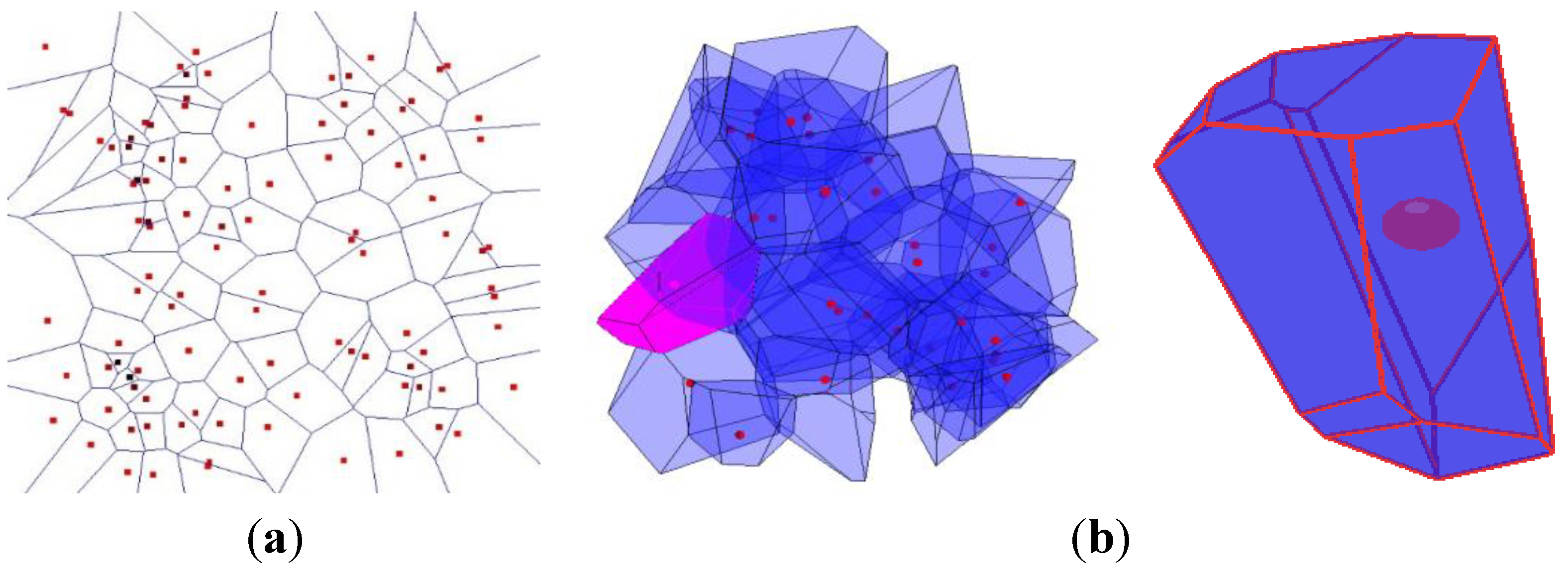
2.1. Definition and Description of 3D Voronoi Diagram

A three-dimensional Voronoi diagram divides the 3D points into convex polyhedrons such that each polyhedron contains exactly one particle (the generating 3D point), and every point in a given Voronoi cell is much closer to the generating point than to any other generating points in the space.

Let the expression P = {p₁, p₂, p₃…}$\subset R^3$ represent a locally finite point set with C(P) = $R^3$, where C(P) denotes the convex hull of the family P. Then, the Voronoi diagram V induced by P is defined by the nearest–neighbor principle, i.e., the cells $\left\{VCel{l}_i\right\}$ of VD are given by the following expression:

$$VCel{l}_i=\left\{p\in R^3:\left|p-p_i\right|\le \left|p-p_j\right|\right\} \text{for all} \text{i}\ne \text{j}$$

(1)

Notably, $VCel{l}_i$ can be represented as a convex polyhedron that is bound and locally finite in a 3D space or in an intersection of half-planes in a 2D space. Because P is locally finite, it is clear that the cells have a non–empty interior. Moreover, their union covers $R^3$, and two different cells can only touch at their boundaries. Thus, the family $C\left(P\right)=\left\{VCel{l}_i\right\}$ constructed in this manner is a diagram. A 2D Voronoi diagram and the voxel shape of a single 3D Voronoi cell from a 3D Voronoi diagram along with the generating points are displayed in Figure 1.

Figure 1. Two-dimensional Voronoi diagram (a) and 3D Voronoi diagram/cell (b).

Figure 1. Two-dimensional Voronoi diagram (a) and 3D Voronoi diagram/cell (b).

Many parameters can describe an individual 3D Voronoi cell. This study uses the following parameters, as depicted in Table 1: the particle’s coordinate, identifier, facet #, surface area, volume of the 3D Voronoi cell, 1-order neighbors of a certain cell and global depth of a certain cell in the Voronoi diagram. The former five parameters (i.e., particle’s coordinate, identifier, facet # and surface area, and volume of the 3D Voronoi cell) describe the individual characteristics of the Voronoi cell, and the latter two parameters (i.e., 1-order neighbors and depth), which are explained in Section 2.2, depict the spatial relationships of a given Voronoi cell in Voronoi diagram. These parameters of a Voronoi cell consider both the cell itself and its context in Voronoi diagram. Additionally, before the 3D Voronoi diagram is constructed, we should determine the outer box of the domain and consider the edge effects of the Voronoi cell near the box’s boundary.

Each stationary random Diagram C(P) in $R^3$ induces stationary random lower-dimensional manifold processes. The 3D Voronoi cell is related to the point process of facets. Every particle’s birth or death results in a change in the local structure for a 3D Voronoi diagram. This local change and update can facilitate the local clustering and segmentation of points within a Voronoi diagram to reduce the computations. Figure 2 shows the birth and death processes of one particle, represented by a 3D sphere in a certain radius (Figure 2a), along with the corresponding 3D Voronoi diagram (Figure 2b).

Table 1. Description of the 3D Voronoi cell parameters.

Parameter	Description	Note
Particle	The generating point	3D coordinate
ID	Identifier of the Voronoi cell	Integral number
Facet #	The number of facets of the given Voronoi cell	Degree that indicates the number of spatial neighbors
Surface area	Surface area of the given Voronoi cell	Related to tension and density
Volume	Volume of the given Voronoi cell	Related to tension and density
1-order neighbors	Direct neighbors of the given cell	The cells share facets with the given cell
Depth	Depth of N-order neighbors of the given cell	Globe depth of multiple order neighbors in 3D Voronoi diagram or within a cluster

Table 1. Description of the 3D Voronoi cell parameters.

Parameter	Description	Note
Particle	The generating point	3D coordinate
ID	Identifier of the Voronoi cell	Integral number
Facet #	The number of facets of the given Voronoi cell	Degree that indicates the number of spatial neighbors
Surface area	Surface area of the given Voronoi cell	Related to tension and density
Volume	Volume of the given Voronoi cell	Related to tension and density
1-order neighbors	Direct neighbors of the given cell	The cells share facets with the given cell
Depth	Depth of N-order neighbors of the given cell	Globe depth of multiple order neighbors in 3D Voronoi diagram or within a cluster

Figure 2. Spatial birth-and-death processes: (a) 3D points; (b) the corresponding 3D Voronoi cells.

Figure 2. Spatial birth-and-death processes: (a) 3D points; (b) the corresponding 3D Voronoi cells.

2.2. Spatial Neighborhood Relationships of 3D Voronoi Cells

A three-dimensional Voronoi diagram is an efficient method for describing spatial distributions using the spatial neighbor relationships among spatial points [16,33]. The topological neighbors of 3D Voronoi cells provide candidates that interact with the given cell and exert vital influence on the spatial pattern during the clustering process. The multiple order (N-order) neighbor property is an important feature of a Voronoi diagram. All of the neighbor cells that share facets are recorded through the construction process of the Voronoi diagram. With topological representation of the Voronoi cell, the direct neighbor cells of each Voronoi cell can be conveniently extracted. Voronoi cells that directly share facets with the cell of given particles are denoted by 1-order neighbors, and 2-order neighbors refer to the cell/particles that are 1-order neighbors of the prior 1-order sets of particles (the previous neighbor cells are exclude in the new neighbors), and so on. The depth of spatial order indicates how deep the order of one certain cell could be in the overall Voronoi diagram. Thus, the gradual cumulative near neighbors of a certain particle can be extracted according to the n-order neighbor relationships.

Within a set of 100 particles (Figure 3a), the boundary face in a red Voronoi cell represents the spatial partition of a certain selected particle (Figure 3b) with ID 33 at the corner of the cube. This Voronoi cell has 10 facets, indicating that it has ten 1-order neighbor cells in the Voronoi diagram, as shown in Figure 3a and Table 2, including three boundary faces without neighbors. This Voronoi cell has a total depth of 4-order in this diagram, and more cumulative 4-order neighbors with identifiers are displayed in Table 2 and shown in Figure 3a, which for illustration purposes, uses different colors, from red to blue, to dye the particles and Voronoi cells and to show the 4-order neighborhood relationships in the three-dimensional spatial point patterns. A slicing profile crossing the selected cell illustrates the gradual neighbor in different colors in Figure 3c.

Figure 3. 4-order neighbors in the 3D Voronoi diagram of 100 particles (a) with the highlighted one at the corner (b) and a slicing profile crossing the highlighted one to show the gradual neighbor relationships in 2D (c).

Figure 3. 4-order neighbors in the 3D Voronoi diagram of 100 particles (a) with the highlighted one at the corner (b) and a slicing profile crossing the highlighted one to show the gradual neighbor relationships in 2D (c).

Table 2. N-order neighbors of a certain particle in a 3D Voronoi Diagram.

n-order	Particle ID	Number of Neighbors
1	94,88,46,23,16,45,72,4,50,61	10
2	7,92,84,68,82,80,30,8,93,57,18,81,90,9,12,19,59,13,98,79,75,3,99,41,2,44,65,97,55,91,62,32,87	34
3	70,67,52,64,11,53,36,0,96,73,21,27,5,40,95,39,25,35,34,17,14,56,49,51,28,38,31,10,6,24,78,76,85,63,1,89,69,29,77,20	40
4	26,37,42,58,74,22,60,71,83,43,66,15,48,86,54,47	10

Table 2. N-order neighbors of a certain particle in a 3D Voronoi Diagram.

n-order	Particle ID	Number of Neighbors
1	94,88,46,23,16,45,72,4,50,61	10
2	7,92,84,68,82,80,30,8,93,57,18,81,90,9,12,19,59,13,98,79,75,3,99,41,2,44,65,97,55,91,62,32,87	34
3	70,67,52,64,11,53,36,0,96,73,21,27,5,40,95,39,25,35,34,17,14,56,49,51,28,38,31,10,6,24,78,76,85,63,1,89,69,29,77,20	40
4	26,37,42,58,74,22,60,71,83,43,66,15,48,86,54,47	10

Gradual cumulative neighbors resulting from one certain particle can be used as a model of complete candidate particles that can be compared with the importance value during the clustering process.

The definition of a point neighbor is used in our method with the following advantages: (1) it is scale-independent and can be adapted to the scale and spatial density so that we can address the point cloud regardless of the point number and point range; (2) in contrast to other parameters with specific values, a spatial neighbor only indicates the spatial order of the neighborhood, and the neighbor relationships are symmetric with each other, which can support the holistic spatial distribution analysis of the point cloud; (3) a 3D scatter point cluster based on a 3D Voronoi diagram can also segment the point cloud with the same effects as surface convex decomposition (e.g., [23]).

2.3. Measurements in the Voronoi Method

Importance Value

To implement point clustering and point cloud segmentation, each particle should have an importance value to indicate its power in the context of the 3D Voronoi diagram. The clustering method in this study is based on a hierarchical cluster of the similarity (for related contents, refer to the cited literature), but the importance is not merely delimited by a normal Euclidean distance. As stated in Section 2.2, a 3D Voronoi diagram can provide the spatial partition of particles, and many parameters can be used to describe the 3D Voronoi cell. The principle of clustering depends on the definition of spatial relationships and the importance on each particle. In addition to the Euclidean distance, simple definitions of importance can be employed by the volume and the surface area or its reciprocals of a 3D Voronoi cell, which contains the source point. Additionally, in this study, the multiple importance values are defined based on the above parameters. The importance of a Voronoi cell can be the combination of these parameters, for example, the 3D density of a Voronoi diagram can be described by Equation (2). These parameters can reflect the density importance of each point. The importance value can be calculated using a relative reference, as in Equations (2) and (3). From Equation (3), it can be indicated that the relative importance values are directed and not symmetric with each other.

$$r_i=d_k\left(i\right)/{{\displaystyle \sum }}_{i=1}^{n}d\left(i\right)$$

(2)

where $d_k$ refers to the parameters (by the volume and the surface area or its reciprocals of a 3D Voronoi cell).

$$wr\left(i,j\right)=r\left(i\right)/\left(r\left(i\right)+r\left(j\right)\right)$$

(3)

Classical cluster theory reveals that the 3D spatial distributions of homogeneous particles/cells, assuming coalescence or cell growth, follow the clustering process. The conventional cluster is based on a point-to-point distance to group the nearest particles/cells. Using the parameters of the 3D Voronoi cell, each particle can be assigned a certain importance according to its volume, surface area or their reciprocal and their combination (Equations (2) and (3)). In actual applications, a certain density or tension can be imposed on the 3D Voronoi cell to control these parameters [18].

Spatial Neighborhood Relationship

More importantly, spatial neighborhood relationships of 3D Voronoi cells support the point cluster during computation. A higher number of neighbors and the closer the points are, the more likely the points are clustered and segmented together. The spatial neighborhood relationship is stated in Section 2.2.

The 1-order cell aggregation of the particle i can be formulated by the following equation:

$$C^1\left(p_i\right)=\underset{j:j\in neibr\left(i\right)}{{\displaystyle \cup }}{C}_j{\cup }^{\text{}}C\left(p_i\right)$$

(4)

Therefore, $C_j$ is the spatial neighbor of the Voronoi cell of particle i.

When this neighborhood relationship is considered, the similarity between the 3D points can be confirmed by the neighborhood relationships. Clustering only occurs on the neighbor cells and passes on to them. Apparently, the operation of particle aggregations is sequentially associative; thus, we can perform this operation gradually according to the neighborhood relationships to determine the different spatial patterns of the particles. Thus, the resultant Voronoi cell clusters include all of the close 3D points and their neighbors.

Particle Statistics

The number of points that are aggregated together as a cluster are calculated to indicate the segmentation of the point cloud.

Depth of the Cluster

The maximal order of the neighborhood in a cluster is the depth of the cluster, which indicates how deep the points are clustered together through topologic neighbor relationships.

3. Point Cluster Analysis Using the 3D Voronoi Diagram and Applications in Point Cloud Segmentation

The quantitative features of 3D Voronoi cells that aid in the measurement of both the local structure of the individual cell and the global topology the 3D Voronoi diagram are extracted, as described in Section 2.1 and Section 2.2. Moreover, the trends of these features can be controlled by manipulating the point clusters through the cell density according to their parameters. As described previously, the 3D Voronoi cell responsible for the particle recorded in each importance value is identified based on the spatial properties of the parameters, and the interactions are confirmed by the correlation among the individual particles. These characteristics can be utilized to implement and analyze the point cloud clusters and segmentations of 3D models, which are discussed in this section. This section describes the clustering process with the aid of different importance values based on the 3D models and stationary scatter point sets. During the clustering process, the particles remain stationary and are divided into different classes and then clustered together.

3.1. Method Procedures

To illustrate the feasibility of our method, different 3D point clouds are tested to cluster and segment the 3D Voronoi diagram by cluster. Clustering procedures include the following steps:

(1)

Construct the 3D Voronoi diagram of a 3D point cloud;

(2)

Compute the parameters of each 3D Voronoi cell and its neighbor cells; and

(3)

Cluster 3D points with a given number of clusters by hierarchical cluster and Voronoi parameters (Section 3.2).

The distance between 3D points is calculated within point $p_0$ and its 1-order neighbor set; thus, the minimum distance is as shown in Equation (5):

$$D_0=d\left(C^1\left(p_0\right),p_0\right)=\underset{1<j<m}{\min }(p_j,p_0)$$

(5)

Using the hierarchical cluster, the distance between the p cluster class and the q cluster class is calculated with the following formula, and the further recursion formula for the k cluster class compared with the (p + q) cluster class is given in Equations (6) and (7):

$$D_{pq}^2=\frac{1}{n_p{n}_q}{\displaystyle \sum }_{i\in G_p}{\displaystyle \sum }_{i\in G_q}{d}_{ij}^2$$

(6)

$$D_{pq}^2=\frac{n_p}{n_p+n_q}{D}_{kp}^2+\frac{n_q}{n_p+n_q}{D}_{kp}^2$$

(7)

Through these formulas, the cluster proceedings are performed, and the results are listed in the following applications and tests.

3.2. Random Point Cluster Analysis Based on 3D Voronoi Diagrams

In this section, the Euclidean distance, importance value and spatial neighborhood relationship between the particles are calculated with case studies such that the farthest particles can be included in the neighborhoods, and the difference from random scattering diminishes.

To test the cluster differences and the universality of the results regarding this approach using the different parameters, we establish a 3D Voronoi cell to show the structure and spatial pattern of the random spatial 3D points, and clustering methods are based on the interactions among the particles corresponding to their neighbor relationships. Spatial clusters and their distributions of particles with the same cluster number are different according to different parameters, as indicated in Section 2.1 and Section 2.3. Suppose that 1000 particles should be classified into 100 clusters in the test; represented by the colors of the particles’ spheres, the result in Figure 4a shows that the scattering of the spatial distributions is only according to the density related to the volume of the 3D Voronoi cells, while Figure 4b displays the grouping and assembly of spatial distributions under the consideration of neighborhoods of 3D Voronoi cells for the same cluster number.

Figure 4. Different clusters and their distributions of particles for the same cluster number: (a) scattering without neighbor relationships; (b) clustering with neighbor relationships.

Figure 4. Different clusters and their distributions of particles for the same cluster number: (a) scattering without neighbor relationships; (b) clustering with neighbor relationships.

Additional cases are tested to examine the spatial pattern of random points’ clustering with different importance values based on the 3D Voronoi diagram. Sample stationary points include 1000 particles, and four different importance values are used in cluster processes within 10 cluster classes. Figure 5 gives the point patterns of different spatial distributions according to the different importance values, and the differences of the numbers of the Voronoi cells of each class in the cluster pattern are listed in Figure 6.

Figure 5. Different patterns according to different importance values: (a) surface area. (b) neighborhood and distance; (c) neighborhood + distance + volume; (d) neighborhood + distance + surface area.

Figure 5. Different patterns according to different importance values: (a) surface area. (b) neighborhood and distance; (c) neighborhood + distance + volume; (d) neighborhood + distance + surface area.

The tested particles were classified into 10 classes based only on the surface area of the corresponding Voronoi cells, as shown in Figure 5a, and it can be found that the particles of each cluster class disperse and do not aggregate in the cube. Compared with this scatter characteristic of clustering without neighborhood relationships, as shown in Figure 5a, the results of the other three cluster analyses illustrate the characteristics of spatial group distributions under the neighbor relationships separately with the addition of normal distance (Figure 5b), distance and volume of the Voronoi cell (Figure 5c), and distance and surface of the Voronoi cell (Figure 5d). To highlight the visual effects of the spatial distribution of the particles, only the particles with different colors, which indicate their different classes, are depicted in Figure 5a–d, and the corresponding Voronoi cells are hidden to facilitate visualization.

Figure 6. Statistics of the number of particles in 10 classes with different importance values.

Figure 6. Statistics of the number of particles in 10 classes with different importance values.

In Figure 6, three curves indicate the similar number of particles in each cluster class among the three clustering processes in which all are based on neighborhood relationships along with other parameters, which is different from the process based on the individual parameter of the surface area of the particles, depicted in blue. It can be indicated that among the clusters with neighborhood relationships (i.e., Neighborhood + Distance cluster, Neighborhood + Distance + Volume cluster and Neighborhood + Distance + Surface area cluster), the difference in particle number in the same cluster class is small because of the Voronoi neighborhood results in the balance of spatial point distributions between the different cluster classes; this difference is large between the cluster with “surface area” and the other three clusters because without spatial neighborhood relationships, the centrality of the spatial point distribution within one cluster class is very weak, and randomness increases. Tens of tests on random point sets show similar consequences in which the spatial neighbor relationships play a vital role in 3D point clustering.

Figure 6 and Figure 7 show the clustering results with different thresholds for the distance. “Close” and “neighbor” are not mutually equal. The tests show that the neighborhood relationship has a direct effect on the cluster results, especially the distribution of clustering points. The spatial neighborhood relationship leads to continuous clusters that are reliable for segmenting the parts of the 3D body in Section 3.3.

Figure 7. Simulation of continuous clustering progression in different cluster numbers based on Euclidean distance and neighbor relationship: (a) 1000; (b) 500; (c) 250; (d) 125; (e) 60; (f) 30; (g) 10; and (h) 5.

Figure 7. Simulation of continuous clustering progression in different cluster numbers based on Euclidean distance and neighbor relationship: (a) 1000; (b) 500; (c) 250; (d) 125; (e) 60; (f) 30; (g) 10; and (h) 5.

The clusters selected for analysis have some interactive importance value of influence between them. Each particle interacts with its spatial neighbor particles to attempt to polymerize them when the cluster process among the particles begins. Because every 3D Voronoi cell is surrounded by its nearest (1-order) neighbor cells iteratively, the interactions among the particles appear as a continuous changing process. During this process, all of the particles are independent of and homogenous with each other; their parameters, importance values and neighborhood per iteration are updated, and the number of clusters is checked to implement the cluster.

Interactive visualization of 3D spatial points based on the 3D Voronoi diagram can simulate and explain the processes of some phenomena [34], including blood [19], galaxies [1,3,35], and porous materials [36], among others. We can also present the spatial and temporal analysis of the evolution of spatial 3D particles with the stationary mode. The progression of the process is dependent on the parameters or importance values of the spatial particles and represents direct, cell-based changes that can be simulated through time and space. Here, we simulate the progress of the cluster. The cluster manner shown in Figure 7 visualizes the continuous hierarchical clusters of spatial particles, based on the Euclidean distance and neighbor relationship, according to the different cluster class numbers and the corresponding spatial distribution patterns.

By comparing the clustering based on one parameter (e.g., surface area in Figure 5a), the neighborhood and their combination (see Figure 4b and Figure 5), as well as the progressive cluster of 3D particles with regard to spatial neighborhood relationships (Figure 7), the effects of the spatial cluster based on the Voronoi diagram can be directly visualized. Using the multiple order (N-order) neighborhood approach based on the 3D Voronoi diagram, the intensity of the spatial 3D point clustering could strengthen with regard to the spatial neighbors. Because the cluster reflects the local spatial configuration of the particles in 3D space, it is relatively insensitive to variations in density and the dimensionality of the space, which promotes the clustering stability.

We utilize the spatial neighborhood relationship to define the cluster, to reveal that the significant features of a spatial pattern do exist in the process of clustering and to show that these features represent the connectivity and modularity of the spatial distribution. These characteristics are utilized to segment 3D point clouds with the tests described in Section 3.2.

3.3. Applications in Point Cloud Segmentation of 3D Models

The clustering and segmentation of a 3D point cloud aim to divide the 3D points into several coherent and consecutive subsets, and after the segmentation, the subsets of the 3D points have a certain similarity, function, or spatial distribution, which is the foundation of the segmentations of a 3D point cloud.

Test 3D point cloud data are from the Stanford 3D Scanning Repository (http://graphics.stanford.edu/data/3Dscanrep). These data include point clouds for 3D models of a Horse, Cow, Armadillo, Deer, Camel, Horse, Elephant and Hand.

Their point clouds describe the 3D surfaces of their body shapes, and the configurations of the 3D points show a certain regular distribution. It is difficult to cluster 3D points and to segment them based on the normal distance parameter. We construct 3D Voronoi diagrams for them and calculate the parameters of each Voronoi cell. The spatial neighborhood relationship, distance, and density are used to cluster the 3D homogeneous points and form the segmentation of the 3D body components/parts of the 3D models. To clearly visualize the 3D points, the points in the point cloud, for example, the 3D horse with 2483 particles in Figure 8a, are enlarged into a ball to the show distinct 3D body shape, and the 3D Voronoi cells about the 3D particles of the horse are illustrated in Figure 8b.

Clusters and segmentations of the horse with cluster numbers of 2, 3, 4, 5, 6 and 8 are shown in Figure 9, and Table 3 lists the body components and point number in each cluster class. It is easy to identify the horse’s body components with different cluster numbers. For example, for three clusters, the horse is segmented into head, front legs and half rear body, and further, for 8 clusters, front feet, rear feet, horseback and withers are clearly recognized.

Figure 8. 3D point cloud of the Horse (a) and its 3D Voronoi diagram (b).

Figure 8. 3D point cloud of the Horse (a) and its 3D Voronoi diagram (b).

Figure 9. Illustrations of clustering and segmentation of the Horse point cloud with different cluster numbers: (a) 2; (b) 3; (c) 4; (d) 5; (e) 6 and (f) 8.

Figure 9. Illustrations of clustering and segmentation of the Horse point cloud with different cluster numbers: (a) 2; (b) 3; (c) 4; (d) 5; (e) 6 and (f) 8.

The results in Table 3 indicate that the maximal holistic depth of the horse point clouds is 12, and the depths of the clusters are nearly as close. It can be concluded that from the segmentations and depth of the Voronoi neighborhood in 5 clusters and 8 clusters, each cluster has strong centrality and convergency to cluster the neighbors together. In addition, the spatial point distributions of each component of the Horse include a different number of points but a similar depth of the spatial neighborhood.

Table 3. Horse clustering and segmentation.

Number of Clusters	Number of 3D Points	Max. Depth of Cluster	Body Components
1	2483	12	Body
2	1234	12	Half front body
	1249	11	Half rear body
3	683	10	Head and neck
	566	10	Front leg
	1234	12	Half rear body
4	683	10	Head and neck
	566	10	Front leg
	226	8	Rear feet
	1008	9	Half rear body
5	279	8	Withers
	566	9	Front leg
	226	8	Rear feet
	1008	9	Half rear body
	404	8	Head
6	279	8	Withers
	566	9	Front leg
	226	8	Rear feet
	676	9	Crupper
	332	9	Horseback
	404	8	Head
8	279	8	Withers
	169	8	Front feet
	226	8	Rear feet
	397	9	Front leg
	676	9	Crupper
	160	8	Horseback
	172	8	Belly
	404	8	Head

Table 3. Horse clustering and segmentation.

Number of Clusters	Number of 3D Points	Max. Depth of Cluster	Body Components
1	2483	12	Body
2	1234	12	Half front body
	1249	11	Half rear body
3	683	10	Head and neck
	566	10	Front leg
	1234	12	Half rear body
4	683	10	Head and neck
	566	10	Front leg
	226	8	Rear feet
	1008	9	Half rear body
5	279	8	Withers
	566	9	Front leg
	226	8	Rear feet
	1008	9	Half rear body
	404	8	Head
6	279	8	Withers
	566	9	Front leg
	226	8	Rear feet
	676	9	Crupper
	332	9	Horseback
	404	8	Head
8	279	8	Withers
	169	8	Front feet
	226	8	Rear feet
	397	9	Front leg
	676	9	Crupper
	160	8	Horseback
	172	8	Belly
	404	8	Head

To demonstrate the approach’s feasibility, additional point clouds of the 3D models (i.e., Cow, Armadillo, Deer, Camel, Horse, Elephant and Hand) are tested. Table 4 presents the segmentation results generated by our approach for different 3D models. It can be concluded that the approach effectively clusters the 3D point clouds and successfully decomposes concrete body components. Our experiments on various 3D models demonstrate that our algorithm possesses the desirable properties of stability, reliability, and robustness.

Table 4. Segmentation results with different cluster class numbers.

3D Model (# Point)	Cluster Number (Parts of 3D Models)
	2	3	4	5	6
Fish 2366
Armadillo 2742
Deer 3033
Camel 2443
Elephant 2775
Hand 1055

Table 4. Segmentation results with different cluster class numbers.

3D Model (# Point)	Cluster Number (Parts of 3D Models)
	2	3	4	5	6
Fish 2366
Armadillo 2742
Deer 3033
Camel 2443
Elephant 2775
Hand 1055

3.4. Discussion

The parameters exert different influences on the point clusters based on the 3D Voronoi diagram. The segmentation results from different models show that the segmentations using our approach are reliable for 3D point clouds. It is also apparent that the segmentations depend on the clustering of 3D point distributions, which is determined by three parameters: distance, importance value and spatial neighborhood relationship. The spatial neighborhood relationship is responsible for selecting the candidate clustering points. The distance is determined by the span of the points, along with certain importance values, and is responsible for the cluster.

The method does not depend on the point itself or on plane features but on the 3D distribution and the spatial 3D neighborhood relationships to group other 3D points, which improves the segmentation of the point cloud and overcomes the disadvantage of clustering based on normal distance in which it is difficult to select the closest point to a group. The proposed method is also applicable for segmenting other 3D models with 3D scattering points. The limitation of our method is that for 2D or 2.5D point clouds (e.g., terrain), our method may overlook the computation and cause inaccurate results due to the full 3D computation. Another limitation of our method is the over-segmentation of some components because of their self-touch or neighbor relationships between different components, which may produce inconsistent results. For example, the hand in Table 4 with 4 clusters can be consistent with joint of the figures; which in 5 and 6 clusters, but the segmentations are not consistent with each figure or joint of the figure. A possible solution is to further constrain surface clustering during segmentation; there is no surface in our method, and only 3D points are considered. The performance of the algorithm depends on the number of the 3D points and the different parameters, that is, different parameter has different computations and different complexity.

There are several advantages of our 3D Voronoi cell approach for analyzing point patterns. First, the 3D Voronoi diagram is not restricted to 2D planar points, which can provide a precise mathematical representation and simulate their 3D spatial structure, and it is insensitive to the scale and range of point clouds. Furthermore, 3D Voronoi cells enable us to benefit from different parameters and their variations and provide a flexible method to describe the importance values of each particle in the cluster process, which extends and facilitates its applications, such as for proteins and galaxies. Third, each 3D Voronoi cell has several facets, indicating many spatial neighbor cells and N-order neighbors; thus, spatial clusters can be implemented according to spatial neighborhood relationships to approach the actual situations. The proposed method reaches the segmentations of the point clouds of 3D models, which is completely different from most of the mesh decompositions or surface decompositions of 3D models. The results can be further used as surface decompositions with additional surface modeling.

4. Conclusion

3D point pattern analysis and its clustering focus on the spatial analysis of points corresponding to Voronoi cells in our case, whereas to define the “spatial structure”, one must model cell-cell (point-to-point) relationships. The 3D Voronoi diagram provides an efficient method to determine the potential spatial distribution and neighborhood relationships, constituting an approach to evaluate the similarity of point sets and to enhance point clusters and point cloud segmentation. 3D Voronoi cells allow for the existence of facets between adjacent cells such that only the spatial neighbor particles can be clustered into one class during the clustering model. These analyses integrate the normal parameters (distance, surface area and volume) with spatial neighbor relationships to enhance the inherent relationships among individual Voronoi cells. The experiments showed that the proposed method is robust regarding the shape and distribution of 3D points, which provide the foundation of surface structure, point cloud compression and feature detection and extraction.

References

1. Panko, E.; Flin, P. Application of the Voronoi tessellation technique for galaxy cluster search in the Münster Red Sky Survey. Proc. Int. Astron. Union Colloq. 2004, 2004, 245–247. [Google Scholar] [CrossRef]
2. Ramella, M.; Boschin, W.; Fadda, D.; Nonino, M. Finding galaxy clusters using Voronoi tessellations. Astron. Astrophys. 2001, 368, 776–786. [Google Scholar] [CrossRef]
3. Elyiv, A.; Melnyk, O.; Vavilova, I. High-order 3D Voronoi tessellation for identifying isolated galaxies, pairs and triplets. Mon. Not. R. Astron. Soc. 2009, 394, 1409–1418. [Google Scholar] [CrossRef]
4. Dupuis, F.; Sadoc, J.F.; Mornon, J.P. Protein secondary structure assignment through Voronoi tessellation. Proteins. 2004, 55, 519–528. [Google Scholar] [CrossRef] [PubMed]
5. Dupuis, F.; Sadoc, J.F.; Jullien, R.; Angelov, B.; Mornon, J.P. Voro3D: 3D Voronoi tessellations applied to protein structures. Bioinform. 2005, 21, 1715–1716. [Google Scholar] [CrossRef] [PubMed]
6. Gatrell, A.C.; Bailey, T.C.; Diggle, P.J.; Rowlingson, B.S. Spatial point pattern analysis and its application in geographical epidemiology. T. I. Brit. Geogr. 1996, 21, 256–274. [Google Scholar] [CrossRef]
7. Ledoux, H.; Gold, C.M. Modelling three-dimensional geoscientific Fields with the Voronoi diagram and its Dual. Int. J. Geogr. Inf. Sci. 2008, 22, 547–574. [Google Scholar] [CrossRef]
8. Van der Putte, T.; Ledoux, H. Modelling three-dimensional geoscientific datasets with the discrete Voronoi Diagram. In Advances in 3D Geo-Information Sciences, Lecture Notes in Geoinformation and Cartography; Kolbe, T.H., Köning, G., Nagel, C., Eds.; Springer-Verlag: Berlin, Germany, 2011; pp. 227–242. [Google Scholar]
9. Pellerin, J.; Caumon, G.; Julio, C.; Mejia-Herrera, P.; Botella, A. Elements for measuring the complexity of 3D structural models: Connectivity and geometry. Comput. Geosci. 2015, 76, 130–140. [Google Scholar] [CrossRef] [Green Version]
10. Lopreore, C.L.; Bartol, T.M.; Coggan, J.S.; Keller, D.X.; Sosinsky, G.E.; Ellisman, M.H.; Sejnowski, T.J. Computational modeling of three-dimensional electrodiffusion in biological systems: application to the node of ranvier. Biophys. J. 2008, 95, 2624–2635. [Google Scholar] [CrossRef] [PubMed]
11. Jiang, W.; Xu, K.; Cheng, Z.Q.; Martin, R.R.; Dang, G. Curve skeleton extraction by coupled graph contraction and surface clustering. Graph. Models. 2013, 75, 137–148. [Google Scholar] [CrossRef]
12. Widder, E.A.; Johnsen, S. 3D Spatial point patterns of bioluminescent plankton: A map of the “minefield”. J. Plankton. Res. 2000, 22, 409–420. [Google Scholar] [CrossRef]
13. Friedrich, E. The Voronoi Diagram in Structural Optimisation. Master’s thesis, University College London, 2008. [Google Scholar]
14. Yan, H.W.; Weibel, R. An algorithm for point cluster generalization based on the Voronoi diagram. Comput Geosci 2008, 34, 939–954. [Google Scholar] [CrossRef]
15. Mandal, D.A.; Treas, H.E. Parallel processing a three-dimensional free-Lagrange code: A case history. Int. J. High. Perform. C. 1989, 3, 92–99. [Google Scholar] [CrossRef]
16. Ledoux, H. Modelling Three-Dimensional Fields in Geoscience with the Voronoi Diagram and its Dual. Ph.D. Thesis, University of Glamorgan, 2006. [Google Scholar]
17. Dong, P. Lacunarity analysis of raster datasets and 1D, 2D and 3D point patterns. Comput Geosci. 2009, 35, 2100–2110. [Google Scholar] [CrossRef]
18. Hashemi Beni, L.; Mostafavi, M.A.; Pouliot, J.; Gavrilova, M. Toward 3D spatial dynamic field simulation within GIS using kinetic Voronoi diagram and Delaunay tetrahedralization. Int. J. Geogr. Inf. Sci. 2011, 25, 25–50. [Google Scholar] [CrossRef]
19. Wei, Y.; Cotin, S.; Allard, J.; Fang, L.; Pan, C.; Ma, S. Interactive blood-coil simulation in real-time during aneurysm embolization. Comput. Graph. 2011, 35, 422–430. [Google Scholar] [CrossRef] [Green Version]
20. Rosenthal, P.; Linsen, L. Enclosing surfaces for point clusters using 3D discrete Voronoi Diagrams. Comput. Graph. Forum. 2009, 28, 999–1006. [Google Scholar] [CrossRef]
21. Mongrain, J.; Larsen, J. Spatial point pattern analysis applied to bubble nucleation in silicate melts. Comput. Geosci. 2009, 35, 1917–1924. [Google Scholar] [CrossRef]
22. Han, J.; Kamber, M.; Tung, A. Spatial clustering methods in data mining: A survey. Geogr. Data Min. Knowl. Discov. Taylor Fr. 2001, 188–217. [Google Scholar]
23. Mamou, K.; Ghorbel, F. A simple and efficient approach for 3D mesh approximate convex decomposition. In IEEE International Conference on Image Processing, Cairo, Egypt, 7–10 November 2009; pp. 3501–3504.
24. Yang, B.S.; Zhang, Y.F. Automated registration of dense terrestrial laser-scanning point clouds using curves. ISPRS. J. Photogramm. Remote Sens. 2014, 95, 109–121. [Google Scholar] [CrossRef]
25. Shamir, A. A survey on mesh segmentation techniques. Comput. Graph. Forum. 2008, 27, 1539–1556. [Google Scholar] [CrossRef]
26. Hu, R.Z.; Fan, L.B.; Liu, L.G. Co-segmentation of 3D shapes via subspace clustering. Comput. Graph. Forum. 2012, 31, 1703–1713. [Google Scholar] [CrossRef]
27. Liu, Z.B.; Tang, S.C.; Bu, S.H.; Zhang, H. New evaluation metrics for mesh segmentation. Comput. Graph. 2013, 37, 553–564. [Google Scholar] [CrossRef]
28. Liu, X.P.; Zhang, J.; Liu, R.S.; Li, B.; Wang, J.; Gao, J.J. Low-rank 3D mesh segmentation and labeling with structure guiding. Comput. Graph. 2015, 46, 99–109. [Google Scholar] [CrossRef]
29. Boada, I.; Coll, N.; Madern, N.; Sellares, J.A. Approximations of 2D and 3D generalized Voronoi diagrams. Int. J. Comput. Math. 2008, 85, 1003–1022. [Google Scholar] [CrossRef]
30. Okabe, A.; Boots, B.; Sugihara, K.; Chiu, S. Spatial Tessellations: Concepts and Applications of Voronoi Diagrams; John Wiley & Sons: Hoboken, NJ, USA, 2009. [Google Scholar]
31. Ryu, J.; Kim, D.; Cho, Y.; Park, R.; Kim, D.S. Computation of molecular surface using Euclidean Voronoi Diagram. Comput. Des. Appl. 2005, 2, 439–448. [Google Scholar]
32. Hsieh, H.; Tai, W. A simple GPU-based approach for 3D Voronoi diagram construction and visualization. Simul. Model. Pract. Th. 2005, 13, 681–692. [Google Scholar] [CrossRef]
33. Costa, L.F. Voronoi and fractal complex networks and their characterization. Int. J. Mod. Phys. C 2004, 15, 175–183. [Google Scholar] [CrossRef]
34. Borovkov, K.; Odell, D. Simulation studies of some Voronoi point processes. Acta. Appl. Math. 2007, 96, 87–97. [Google Scholar] [CrossRef]
35. Pizarro, D.; Campusano, L.E.; Clowes, R.G.; Virgili, P. Clustering of 3D spatial points using a maximum likelihood estimator over Voronoi Tessellations: Study of the galaxy distribution in redshift space. In Proceedings of the 3rd International Symposium on Voronoi Diagrams in Science and Engineering (ISVD’06), IEEE Computer Society, Banff, AB, Canada, 2–5 July 2006; pp. 112–121.
36. Grau, S.; Verges, E.; Tost, D.; Ayala, D. Exploration of porous structures with illustrative visualizations. Comput. Geosci. 2011, 34, 398–408. [Google Scholar] [CrossRef]