Abstract
Mainland China has become one of the most important markets for international fast-food chains over the past decade. To study the regional spread of KFC and McDonald’s outlets in Chinese cities, the correlation of their distributions and degree of market expansion were explored and compared to analyze both the local and the global spatial autocorrelations. A geographically weighted Poisson regression model was also used to examine the influence of demographic, economic, and geographic factors on their spatial distributions. The findings of this comparative study reveal the site selection criteria at the city level by studying the differences and similarities in outlet distributions for KFC and McDonald’s. The presented results can guide other chains to enhance business location planning and formulate regional development policy.
1. Introduction
Over the past thirty years, retail sales in Mainland China have risen at a steady double-digit growth rate, far surpassing the country’s GDP growth. The boom in the food industry, including the rapid growth in fast-food chains, has also fueled domestic economic growth and expanded employment channels [1,2]. The various favorable factors for investment in China, such as its large population, remarkable socioeconomic development, huge potential market, and good investment environment, have attracted many global fast-food chains, among which KFC and McDonald’s are the most successful in terms of the rate of market expansion. By the end of 2012, the number of KFC outlets in Mainland China had surpassed 4000, and this number has continued to grow by as many as 500 new ones yearly in the past two years. Meanwhile, McDonald’s has opened more than 1700 outlets in Mainland China and is planning to open 600 more over the next two years.
The overseas expansion of the food industry necessitates a comprehensive consideration of many factors such as investment risk, food quality, management strategy, eating habits, and cultural differences [3], which means site selection is vital for success [4,5]. Studies of the distribution of existing chain stores show that traffic network [6], proximity and ethnicity [7,8], household income [9,10,11], and culinary culture [12] all play important roles in the spatial layout of food outlets. Methodologically, multiple regression models are typically used to analyze the locational differences of food stores. Moore et al. [13] used Poisson regression to investigate the relevance of restaurant locations on customers’ racial composition and income, pointing out the decisive impact of ethnic composition and socioeconomic structure on selecting the site of a food store. Powell et al. [14] studied the relations among the racial, ethnic, and income characteristics of customers and the accessibility of fast-food restaurants in the United States using multi-factor regression analysis. They concluded that higher proportions of fast-food restaurants in predominantly black neighborhoods may contribute to racial differences in obesity rates. By adopting a snowball sampling strategy, Larson et al. [15] also examined the relevance of the locational disparities of grocery stores and fast-food restaurants in the United States for low-income earners, ethnic minorities, and the rural communities. Black et al. [16] used multivariate regression method to estimate the associations between the spatial distribution of food stores and the urban planning and socio-demographic variables in British Columbia. The results indicated that neighborhoods with higher household income had decreased access to food stores.
Despite these findings on the implications of the distribution of food stores, the analyses in previous studies have tended to focus on socioeconomic factors, somewhat overlooking the importance of spatiality. Technically, spatial autocorrelation examines the relationship between similarities and distance [17,18,19]. The phenomenon that near things are more related than distant things is universal. If the relationship is spatially non-stationary, geographically weighted Poisson regression (GWPR) can be used to investigate distributions that are not constant across space [20,21,22,23]. Further, most previous studies have focused on food store distribution within a specific city at the neighborhood level, and few researchers have attempted to investigate the locational differences in the spatial distribution of food stores (especially different international fast-food chains) at the national level, especially in Mainland China. As KFC and McDonald’s, two of the most successful international fast-food chains, compete in all large Chinese cities, it is unclear how they are distributed nationwide and whether there are differences in their layout characteristics. The spatial autocorrelation and spatial non-stationarity of their outlet distributions is worth studying to find out their locational differences and similarities and to understand why they are distributed in this way. These results would benefit the commercial planning processes of other retail chains.
2. Study Area and Data Sources
2.1. Study Area
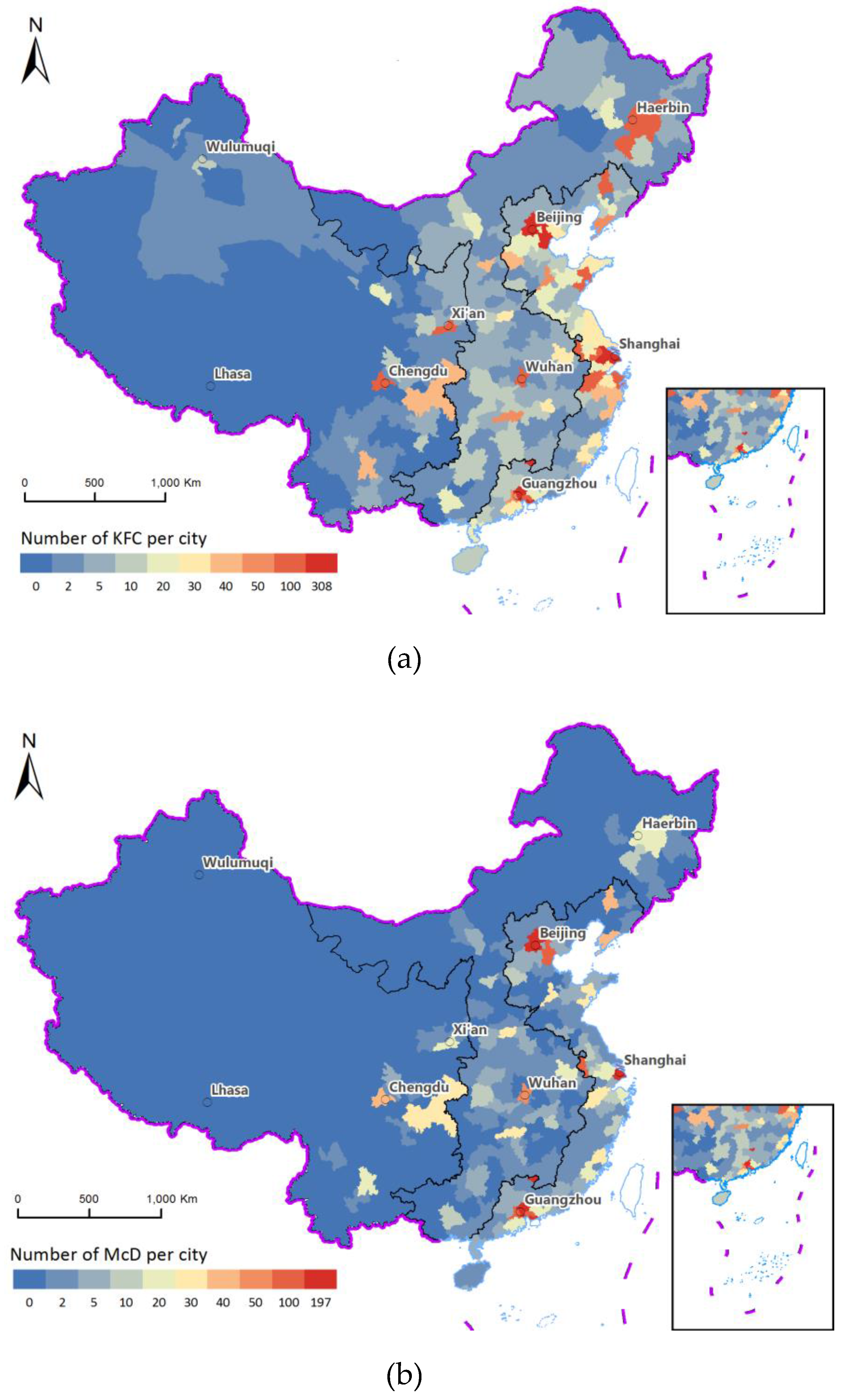
The study area of the present research is restricted to Mainland China only, excluding Hong Kong, Macao, and Taiwan. At the level of prefecture administrative unit, it consists of 337 administrative units at the prefecture level and above. Most KFC and McDonald’s outlets in Mainland China are located in cities. Based on its degree of economic development, Mainland China is traditionally divided into three large regions, namely eastern, central, and western (Figure 1). The eastern region consists of developed coastal provinces, which possess superior natural conditions, convenient transportation links, and remarkable socioeconomic achievement. The central region includes less developed landlocked provinces with large populations and rich natural resources. This is China’s economic hinterland and an important market. The remaining remote undeveloped provinces comprise the western region, which is characterized by harsh natural conditions, high rates of poverty, and narrow markets. In particular, the socioeconomic resources are highly concentrated in the provincial capitals in this region.

Figure 1.
General distribution maps of (a) KFC and (b) McDonald’s outlets.
2.2. Data Sources
The data in this study mainly consist of two types: geographic spatial data and socioeconomic data. The former include the maps of all administrative units in the study area (taken from the National Fundamental Geographic Information System) with the specific locations of KFC and McDonald’s outlets in 2011. The locations of these outlets were collected from the websites of the two fast-food chains and the specifics of the outlets in Mainland China’s major cities were obtained from the corresponding e-maps on the Internet. The latter include the number of permanent residents in the major cities, per capita GDP, and per capita disposable income of urban residents in 2011, which were collected from the China Statistical Yearbook (2012).
3. Spatial Distribution
3.1. General Distribution
The distribution of McDonald’s and KFC outlets decreases from eastern to western China, with a noticeable gap in between, as shown in Figure 1. Approximately 74.1% of KFC outlets (2894) are located in the 12 eastern coastal provinces of Mainland China. Similarly, 80% of McDonald’s outlets (1376) are in these 12 eastern coastal provinces. Large numbers of outlets are concentrated in the Pearl River Delta (centered on Guangzhou), Yangtze River Delta (centered on Shanghai), and Bohai Economic Rim (centered on Beijing). The proportion of KFC and McDonald’s outlets in central China is 17.8% (684) and 14% (236), respectively. Very few outlets are in the western region (KFC 8.1%, 314 outlets; and McDonald’s 6%, 100 outlets). Indeed, McDonald’s has almost no outlets in cities below the level of provincial capital in western China.
As the provincial capital is usually the political and cultural center of a province, the number of KFC outlets in capitals relative to that in ordinary cities reflects the degree of outlet clustering. Table 1 shows the number and percentage of KFC and McDonald’s outlets in the capitals of the three regions. Approximately 71% of KFC outlets in the western region are in capitals compared with 51.6% in central China. Furthermore, while the eastern provinces boast the largest number of KFC outlets, the proportion in capitals is only about 25.8%, far below the average level.

Table 1.
The total number and percentage of KFC and McDonald’s outlets in provincial capitals in the three regions.
With regard to the spatial distribution of outlets for both chains, similarities and differences can be found. In both cases, outlets tend to be concentrated in provincial capitals, while the proportion of outlets in capitals decreases from the west to the east. However, KFC puts more efforts into exploring markets outside capitals, including prefecture-level and county-level cities; its concentration of outlets in capitals is about 10% lower than that of McDonald’s in each region.
3.2. Correlation in Major Cities
The study compared the numbers of KFC and McDonald’s outlets in major cities (provincial capitals and four municipalities). As shown in Figure 2, the regional overlap between KFC and McDonald’s outlets is clear. Beijing, Shanghai, and Guangzhou stand out in the plot as having the largest numbers of outlets. R2 is 0.8774, indicating that cities that have many outlets of one chain also have many outlets of the other. The Spearman’s rho correlation coefficient also reaches 0.907 [24]. Specifically, compared with KFC, the number of McDonald’s outlets in Guangzhou is far above the average level, whereas the number of McDonald’s outlets in Shanghai, Hangzhou, and Harbin is not commensurate with the number of KFC outlets.
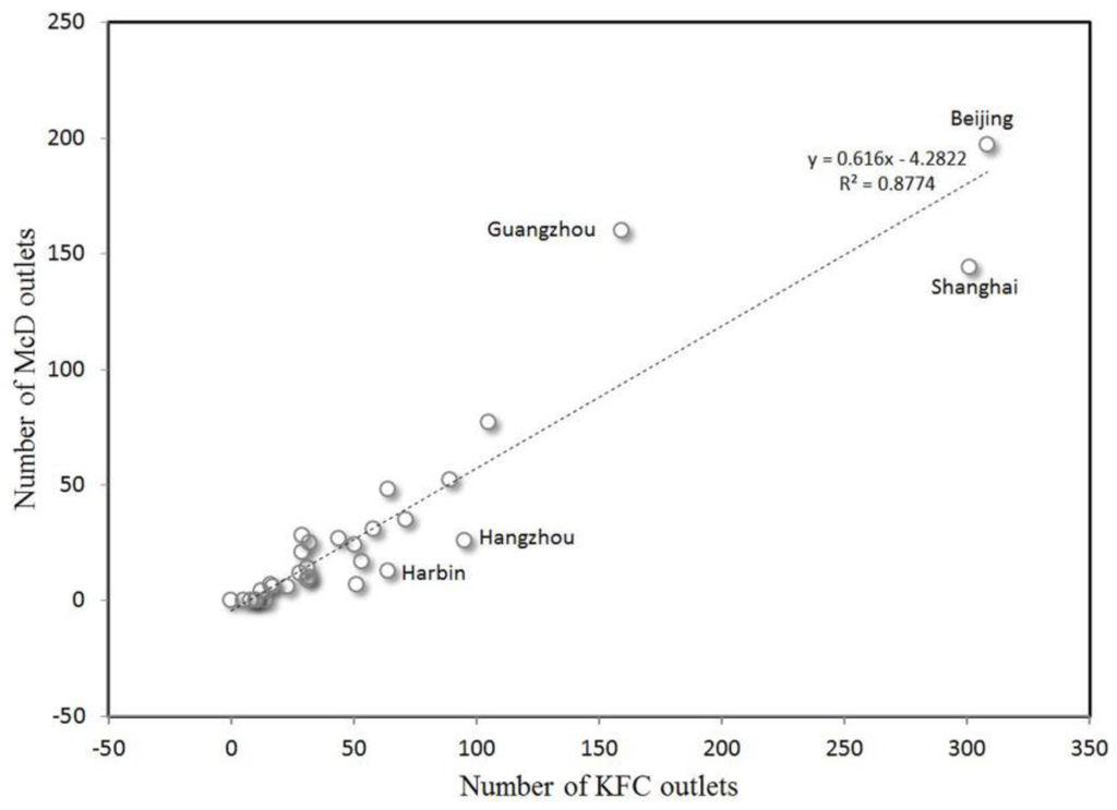
Figure 2.
The comparative plot of KFC and McDonald’s outlets in Mainland China’s major cities.
3.3. Market Expansion
The analysis of market expansion is based on urban grading, which usually grades cities as megacities, extra-large cities, large cities, medium-sized cities, and small cities based on their population size in China. We thus divided the 337 cities above the prefecture level into five tiers, and each tier had a different political status, economic strength, urban scale, and regional attractiveness. The numbers of cities in each tier from top to bottom are 5, 14, 21, 107, and 190, respectively.
The total numbers and average numbers per city of KFC and McDonald’s outlets in each tier of cities are shown in Table 2. The declining trend in the average number of both chains’ outlets in each tier indicates that the degree of the market expansion of their outlets is positively related to urban size. This positive correlation is particularly clear in the case of McDonald’s. In Figure 3, the outlet number at each level of city is divided into several ranges on the x-axis and then the number of cities with outlet numbers included in each range is counted on the y-axis to make the frequency distribution histogram.
Table 2.
The number of KFC and McDonald’s outlets in cities.
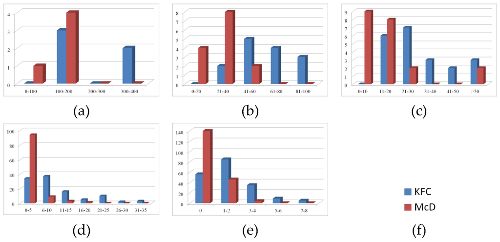
Figure 3.
Frequency distributions of KFC and McDonald’s outlets at the urban grading level for the (a) 1st-tier cities; (b) the2nd-tier cities; (c) the 3rd-tier cities; (d) the 4th-tier cities; and (e) the 5th-tier cities.
Figure 3 shows that KFC covers most cities above the 4th-tier level and 70% of 5th-tier cities. As shown in Figure 3a,b, the number of cities in each range has a relatively small difference, indicating full market expansion by KFC in 1st- and 2nd-tier cities. Inordinately high values, however, appear in Figure 3c,d, showing the great potential for KFC expand to 3rd- and 4th-tier cities despite its widespread coverage there already. This finding accords with the remarkable recent expansion of KFC outlets in 3rd- and 4th-tier cities. By contrast, 5th-tier cities show relatively weak socioeconomic development and consequently they are less capable of attracting investment by international fast-food chains. KFC is known for innovation and adventure in its market expansion strategy (i.e., franchising) in Mainland China, especially in medium-sized and small cities. Further, by grasping the important role of diet culture in China, KFC has applied various localization strategies, such as changing products to adapt to the taste preferences of Chinese consumers, to claim a market-leading position.
The market expansion of McDonald’s lags far behind that of KFC in China. The distribution of McDonald’s outlets covers most 3rd-tier cities and above. However, at the lower level (accounting for 88% of the cities in Mainland China), its market expansion decreases from three quarters (4th-tier) to one quarter (5th-tier) of cities. Figure 3d,e show most cities with 0 or a few outlets, indicating that its market expansion is still in an infancy stage in low-tier cities. In line with its downsizing globally, McDonald’s has shifted its emphasis to 1st- and 2nd-tier cities, thereby broadening the gap between these markets and those in 3rd- to 5th-tier cities. In summary, the different priorities towards market expansion by KFC and McDonald’s have led to their different strategies in this regard.
4. Spatial Autocorrelation Analysis
Spatial autocorrelation aims to detect the degree of correlation between a certain property value or a geographic phenomenon and the corresponding property value or geographic phenomenon of its adjacent locational position on the surface of a geographic area. It can be divided into global spatial autocorrelation and local spatial autocorrelation based on the range of analysis.
Global spatial autocorrelation estimates the spatial distribution of a property value or geographic phenomenon in the overall study area to check whether it is clustering in space. One of the statistics used to evaluate global spatial autocorrelation is Moran’s I index, which measures the correlation of property values in neighboring spatial locations. Local indicators of spatial association (LISA) evaluate the correlation between a property value in a local spatial unit and the corresponding property value in the adjacent area. LISA can be measured by using the local Moran’s I [25]. This can provide more detailed insights into the location of spatial dependence [26]. In addition, a Moran scatter diagram is depicted to visualize the local instability of the property values in the study area. The Moran scatter diagram illustrates the spatial lag factors through a two-dimensional picture and detects the four spatial correlation types in local spatial distribution: high–high (HH), low–high (LH), high–low (HL), and low–low (LL).
4.1. Global Spatial Autocorrelation Analysis
The study used KFC outlets per capita (per million people in this case) to measure the Moran’s I index of global spatial autocorrelation, which is 0.3530. The p value is 0.001, indicating significant global spatial autocorrelation within confidence. Similarly, exploratory spatial data analysis and global spatial autocorrelation were applied to per capita McDonald’s outlets to obtain a Moran’s I of 0.2385 with a p value of 0.001. Each density of the chains’ distribution in different cities thus shows significant positive spatial autocorrelation, which indicates that the spatial distribution does not have a stochastic condition, but rather tends to be adjacent to cities with a higher distribution or lower distribution density.
4.2. Local Spatial Autocorrelation Analysis
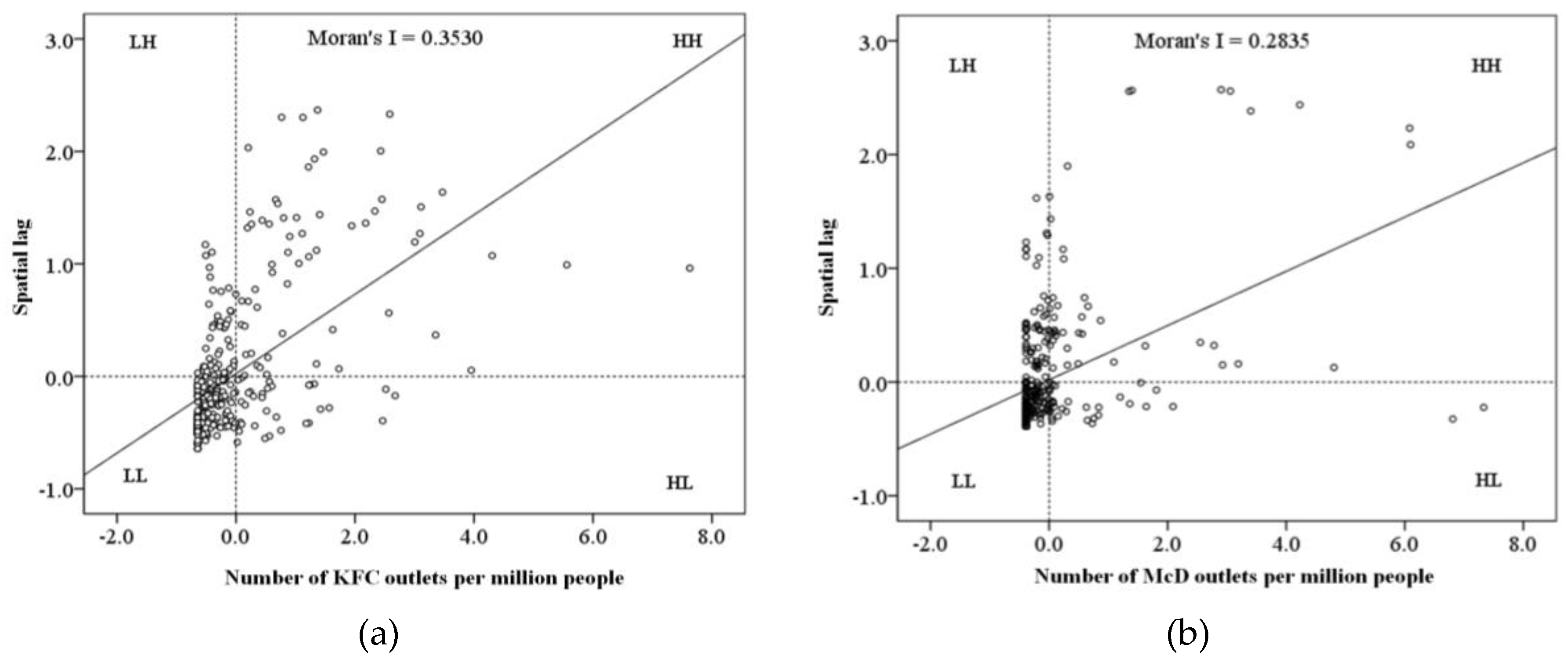
The shortcoming of global spatial autocorrelation is that it often overlooks unusual local conditions or small-scale local instability. Therefore, local spatial autocorrelation is needed to analyze the distribution density of KFC and McDonald’s outlets to reveal their local characteristics (e.g., spatial dependency and heterogeneity). Again, a Moran scatter diagram can be used to evaluate spatial instability within a local range by turning two-dimensional variables into a visualized form. With the normalized average density of the distributions of KFC and McDonald’s outlets as abscissa and spatial lag factors as ordinate, Figure 4 constructs the Moran scatter diagrams for the per capita number of KFC and McDonald’s outlets over the 337 cities in Mainland China.

Figure 4.
Moran scatter diagrams of (a) KFC and (b) McDonald’s outlets.
Figure 4a shows that 256 of the 337 cities are in quadrant 1 (type HH) and quadrant 3 (type LL), indicating that the spatial distribution of KFC does not have stochastic or discrete manner, but rather shows significant positive spatial correlation in the geographic space. This result is consistent with that of the global spatial autocorrelation analysis. The numerous and dense points in quadrant 3 imply that: (i) more cities have a low per capita of KFC outlets compared with a high per capita; and (ii) the low values are closer. The small number of large cities means that the points in quadrant 1 are few and scattered with obvious outliers indicating the disparity of high density values between cities. The distribution of points in quadrants 2 and 4 shows the difference between the cities and their surrounding cities. In quadrant 2 (type LH), 50 atypical cities have a low per capita number of KFC outlets but a high per capita number in their surrounding cities. Moreover, the 31 cities in quadrant 4 (type HL) are unusual in that they have a high per capita number of KFC outlets but a low per capita number in their surrounding cities.
There are 250 points in quadrants 1 and 3 of Figure 4b, indicating significant global spatial correlation in the geospatial distribution of McDonald’s outlets. Compared with KFC, quadrant 1 in the Moran scatter diagram for McDonald’s has fewer, more scattered points; on the contrary, quadrant 3 has more points with a higher density. The scattering of points in the HH zone confirms that the difference in McDonald’s outlets per capita between cities is as considerate as the per capita is high in these cities. The greater number of points in quadrant 3 implies that the market expansion of McDonald’s in Mainland China lags behind that of KFC. In addition, the imbalanced distribution of points in quadrants 2 (59 points) and 4 (28 points) shows a higher number of outliers, indicating the regional disparity caused by McDonald’s insufficient market expansion.
However, while these scatter diagrams display local spatial differences, they provide no index to indicate their significance levels. The measurement of LISA can thus reveal further distribution differences between KFC and McDonald’s. Figure 5 shows the combination of LISA cluster diagrams and Moran scatter diagrams to highlight their differences in spatial distribution.
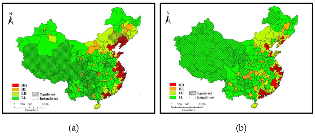
Figure 5.
Local spatial autocorrelation analysis of (a) KFC and (b) McDonald’s outlets.
Significant clustering can be found in the KFC distribution of 139 cities and their neighboring cities at the 5% significance level. Figure 5a shows that fewer cities are characterized with significant HH clustering and these are mainly distributed in the Bohai Economic Rim, Yangtze River Delta, Pearl River Delta, and coastal area in the east of Fujian province. Although Beijing has a high per capita number of KFC outlets, it shows no significant HH clustering because the surrounding cities have a low per capita number. Cities with HL clustering are located mainly in the capitals and well-developed cities in central and western China. Only nine cities have significant HL clustering and these are located in western China. Cities with LH clustering are mainly distributed in the surrounding areas of HH clustering, including the northeast and northwest of the Bohai Economic Rim, the west of the Yangtze River Delta, the west of Fujian, and the northwest of Guangdong. The remaining cities all display LL clustering, with significant clustering in the west.
Although the number of McDonald’s outlets lags far behind that of KFC outlets in Mainland China, its market expansion in Beijing, Shanghai, and Guangdong is comparable with that of KFC. Given that the per capita numbers of both chains are low in western China, the major difference lies in the eastern provinces and central China. Figure 5b shows the different clustering types of McDonald’s outlets. The HH clustering area of McDonald’s covers fewer cities (43) than that of KFC and this difference is particularly marked in the Bohai Economic Rim and the Yangtze River Delta areas. Further, the HH clustering of McDonald’s outlets in eastern coastal areas is not as significant as that of KFC, and some cities here even display HL clustering. By contrast, their adjacent cities in central China show no significant HL clustering, and LH clustering also appears in the surrounding areas. More western areas are characterized with the most significant LL clustering.
5. GWPR Analysis
Regression models are typically built when two or more interdependent quantitative correlations between the independent and dependent variables need to be decided. The geographically weighted regression (GWR) model is an extension of the ordinary linear regression model and this embeds the data locations into the regression parameters [20,27,28]. The regression parameters of certain spatial units used to carry out local regression analysis are no longer arbitrary constants obtained from global information; rather, they come from the measured data of adjacent data and thus vary by spatial location. The main advantage of GWR lies in the use of a distance-weighted data sample to make a point-to-point assessment in the local linear regression analysis. In the case of modeling count responses, Poisson regression models are popular. As a natural extension of GWR, the geographically weighted Poisson regression (GWPR) is thus derived theoretically with geographically varying coefficients using the framework of geographically weighted generalized linear modeling [29].
The spatial statistical analysis with the Moran’s I index and Moran scatter diagram proved the significant spatial autocorrelation in the distributions of the two international fast-food chains. In this section, the GWPR model further explores the driving factors behind the difference in these distributions. We applied the GWR4 software developed by the GWR4 Development Team and a global regression model was executed simultaneously for the comparison [29]. An adaptive Gaussian function was used for kernel type. The Golden Section Search method was chosen to identify the optimal bandwidth size and the AICc was set as the selection criterion. AICc empirically provides better results for Poisson regression [29]. The total number of KFC or McDonald’s outlets was set as the dependent variable in the GWR model, and GDP (G), the per capita disposable income of urban residents (I), and urban population (P) in each city were the independent variables, since these are the most typical and important factors when analyzing the distribution of fast-food chains from a macroscopic perspective.
Table 3 shows the statistical performance of the global regression model and GWPR model for KFC and McDonald’s outlets. Clearly, the GWPR model performs better. To test the spatial heterogeneity of each variable, a semiparametric GWPR model was set, in which one variable was global while the other two variables were local. For KFC outlets, the G, I, and P variables were set as the global term in the semiparametric GWPR #1 (s1), semiparametric GWPR #2 (s2), and semiparametric GWPR #3 (s3) models, respectively. For McDonald’s outlets, the G, I, and P variables were set as the global term in the semiparametric GWPR #4 (s4), semiparametric GWPR #5 (s5), and semiparametric GWPR #6 (s6) models, respectively. The GWPR model has the lowest AICc value for both cases, suggesting that it fits the data the best and there is a spatial non-stationary feature for each variable being examined. We also calculated the spatial autocorrelation of the residual in the two GWPR models. The Moran’s I is 0.073 and 0.048 (p value is 0.001) for the GWPR models of KFC and McDonald’s, respectively, showing that little spatial autocorrelation remains.
Table 3.
Analysis of deviance in models.
In GWPR, the local percent deviance explained (local_pdev) measures the local goodness of fit. The higher the value is, the better the model fits the data. The local_pdev in the KFC GWPR model ranges from 0.758 to 0.903. The mean value is 0.844. The local_pdev in the McDonald’s GWPR model ranges from 0.722 to 0.898. The mean value is 0.814. Therefore, the local goodness of fit is generally good in both GWPR models.
The coefficient of each factor was then calculated in these GWPR models with the minimum, lower quartile, median, upper quartile, maximum, and mean values. The statistical results of the variables G, I, and P are shown in Table 4. The coefficient range of G is (−0.2958, 0.6154), of I is (0.2774, 0.6854), and of P is (−0.1969, 0.6261) in the KFC GWPR model. These three in the McDonald’s GWPR model are (−0.1028, 1.1300), (0.0346, 0.7359), and (−0.4892, 0.5362), respectively. Hence, the coefficient mean values of these three variables tend to be positive. The varying coefficients of G and P indicate the possible existence of both positive and negative correlations in the different areas in the local regression analysis, while the variable I has all positive values in both the KFC and the McDonald’s GWPR models.
Table 4.
Statistics for varying the (local) coefficients.
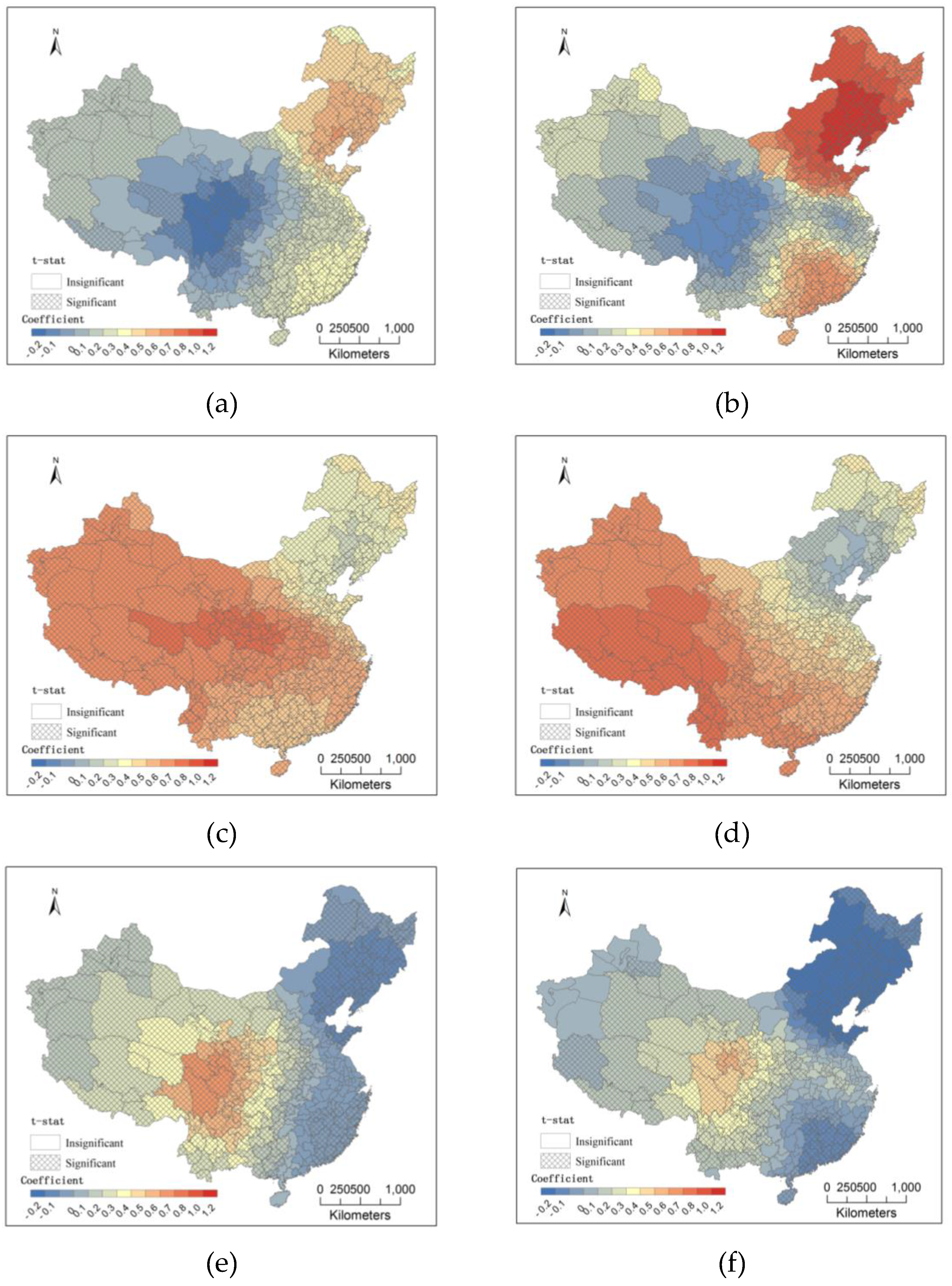
Based on the coefficients of G, I and P in the GWPR models, Figure 6 shows the local correlations between the distribution of outlets and three variables marked with the t-statistical significance. (i) G shows a significant positive correlation in the northeast and a significant negative correlation in the Sichuan Basin in the KFC GWPR model in Figure 6a. Because the rate of urbanization is high and household income gap between cities is low in the northeast, economic size becomes a positive factor driving fast-food chains to open new outlets. One significant difference in distributions between Figure 6a,b is that the southeast area also shows a high value in the McDonald’s GWPR model, which is consistent with the fact that economic development in the Pearl River Delta has quickly grown with the number of McDonald’s outlets; (ii) The coefficients of I decrease from the west to the east (all with positive correlations). Western areas show the largest values, where household income plays an influential role in deciding outlet number by representing consumption capacity. In central China, income is more important to KFC’s decision than to McDonald’s decision, as shown in Figure 6c,d; (iii) P shows a slight impact on deciding outlet location as the mean value is close to zero. However, the positive high values in the Sichuan Basin suggest that the urban population in these areas is a major driving force for fast-food chains opening new markets.

Figure 6.
Regression coefficients of G in (a) KFC and (b) McDonald’s GWPR models; Regression coefficients of I in (c) KFC and (d) McDonald’s GWPR models; Regression coefficients of P in (e) KFC and (f) McDonald’s GWPR models.
6. Conclusions
By taking KFC and McDonald’s as case examples, the paper analyzes the spatial distributions of two international fast-food chains in Mainland China. The spatial distributions of the outlets of both KFC and McDonald’s are generally uneven, decreasing from the eastern to the western regions and expanding from 1st- to 5th-tier cities. Both distributions also display significant clustering. The local Moran scatter plot and LISA analysis indicate that significant HH clustering is distributed in eastern coastal areas for both. LL clustering mostly occurs in the west.
Nonetheless, the distributions of KFC and McDonald’s outlets do differ in some respects. Compared with KFC outlets, McDonald’s outlets are more concentrated in capital cities and they expand more slowly, especially in 3rd- to 5th-tier cities. Further, the LISA analysis indicates that McDonald’s HH clustering includes fewer cities in the eastern region, while LL clustering covers larger areas in central and western China. The relations among the driving factors (i.e., urban population, GDP, and household income) and number of outlets are explored through the construction of the GWPR model. The regression coefficients of the different factors show that the influence on the distributions of KFC and McDonald’s outlets varies at the city level.
The target customers and markets between KFC and McDonald’s overlap since both companies tend to open more outlets in cities with large populations, high household incomes and developed economies. Meanwhile, KFC focuses on developing new markets and McDonald’s on attracting urban youth in large cities. The outlet layouts of the two companies are therefore not the same. The results of the comparative analysis could thus help explain the major driving forces behind the market expansion and site selection criteria of the two companies. Because KFC and McDonald’s are role models from the perspective of business management and location choice of new outlets for other young, ambitious fast-food chains in China, the analysis results can contribute to guide these other chains to enhance business location planning and formulate regional development policy based on their own specific target customers.
Acknowledgments
The authors thank reviewers for their valuable comments and constructive suggestions on this paper. The work was funded by the National Natural Science Foundation of China (41571377), the National Natural Science Foundation of China (41401450), and the General Financial Grant from the China Postdoctoral Science Foundation (2015M571731).
Author Contributions
Yikang Rui and Jiechen Wang conceived and designed the study objective and analysis methods; Huang Huang, Min Lu, and Bao Wang processed the raw data and analyzed the data; and Yikang Rui and Bao Wang wrote the manuscript.
Conflicts of Interest
The authors declare no conflicts of interest.
References
- Luo, D.; Gao, C. An empirical study on the relationship between china’s food trade and economic growth in food industry. In Education and Management; Zhou, M., Ed.; Springer: Berlin, Germany, 2011; pp. 254–259. [Google Scholar]
- Yu, K.; Xin, X.; Guo, P.; Liu, X. Foreign direct investment and china's regional income inequality. Econ. Model. 2011, 28, 1348–1353. [Google Scholar] [CrossRef]
- Bhutta, K.S.; Huq, F.; Frazier, G.; Mohamed, Z. An integrated location, production, distribution and investment model for a multinational corporation. Int. J. Prod. Econ. 2003, 86, 201–216. [Google Scholar] [CrossRef]
- Thomadsen, R. Product positioning and competition: The role of location in the fast food industry. Mark. Sci. 2007, 26, 792–804. [Google Scholar] [CrossRef]
- Nieh, F.-P.; Pong, C.-Y. Key success factors in catering industry management. Actual Probl. Econ. 2012, 130, 423–430. [Google Scholar]
- Ritter, W. Hotel location in big cities. In Big City Tourism; Reimer Verlag: Berlin, Germany, 1986; pp. 355–364. [Google Scholar]
- Eckert, J.; Shetty, S. Food systems, planning and quantifying access: Using GIS to plan for food retail. Appl. Geogr. 2011, 31, 1216–1223. [Google Scholar] [CrossRef]
- Morland, K.; Wing, S.; Roux, A.D.; Poole, C. Neighborhood characteristics associated with the location of food stores and food service places. Am. J. Prev. Med. 2002, 22, 23–29. [Google Scholar] [CrossRef]
- Cummins, S.C.; McKay, L.; MacIntyre, S. Mcdonald’s restaurants and neighborhood deprivation in scotland and england. Am. J. Prev. Med. 2005, 29, 308–310. [Google Scholar] [CrossRef] [PubMed]
- Walker, R.E.; Block, J.; Kawachi, I. The spatial accessibility of fast food restaurants and convenience stores in relation to neighborhood schools. Appl. Spat. Anal. Policy 2014, 7, 169–182. [Google Scholar] [CrossRef]
- Yang, N. March of the Chains: Herding in Restaurant Locations. Available online: https://www.k-state.edu/economics/seminars/retailclusters.pdf (accessed on 12 January 2015).
- Zhang, M.; Wu, W.; Yao, L.; Bai, Y.; Xiong, G. Transnational practices in urban china: Spatiality and localization of western fast food chains. Habitat Int. 2014, 43, 22–31. [Google Scholar] [CrossRef]
- Moore, L.V.; Diez Roux, A.V. Associations of neighborhood characteristics with the location and type of food stores. Am. J. Public Health 2006, 96, 325–331. [Google Scholar] [CrossRef] [PubMed]
- Powell, L.M.; Chaloupka, F.J.; Bao, Y. The availability of fast-food and full-service restaurants in the United States: Associations with neighborhood characteristics. Am. J. Prev. Med. 2007, 33, S240–S245. [Google Scholar] [CrossRef] [PubMed]
- Larson, N.I.; Story, M.T.; Nelson, M.C. Neighborhood environments: Disparities in access to healthy foods in the US. Am. J. Prev. Med. 2009, 36, 74–81. [Google Scholar] [CrossRef] [PubMed]
- Black, J.L.; Carpiano, R.M.; Fleming, S.; Lauster, N. Exploring the distribution of food stores in British Columbia: Associations with neighbourhood socio-demographic factors and urban form. Health Place 2011, 17, 961–970. [Google Scholar] [CrossRef] [PubMed]
- Lopes, S.B.; Brondino, N.C.M.; Rodrigues da Silva, A.N. GIS-based analytical tools for transport planning: Spatial regression models for transportation demand forecast. ISPRS Int. J. Geo-Inf. 2014, 3, 565–583. [Google Scholar] [CrossRef]
- Holloway, P.; Miller, J.A. Exploring spatial scale, autocorrelation and nonstationarity of bird species richness patterns. I ISPRS Int. J. Geo-Inf. 2015, 4, 783–798. [Google Scholar] [CrossRef]
- Cliff, A.D.; Ord, J.K. Spatial Autocorrelation; Pion: London, UK, 1973; p. 178. [Google Scholar]
- Brunsdon, C.; Fotheringham, A.S.; Charlton, M.E. Geographically weighted regression: A method for exploring spatial nonstationarity. Geogr. Anal. 1996, 28, 281–298. [Google Scholar] [CrossRef]
- Yu, D.; Peterson, N.A.; Reid, R.J. Exploring the impact of non-normality on spatial non-stationarity in geographically weighted regression analyses: Tobacco outlet density in New Jersey. GISci. Remote Sens. 2009, 46, 329–346. [Google Scholar] [CrossRef]
- Lu, B.; Charlton, M.; Harris, P.; Fotheringham, A.S. Geographically weighted regression with a non-euclidean distance metric: A case study using hedonic house price data. Int. J. Geogr. Inf. Sci. 2014, 28, 660–681. [Google Scholar] [CrossRef]
- Suárez-Vega, R.; Gutiérrez-Acuña, J.L.; Rodríguez-Díaz, M. Locating a supermarket using a locally calibrated huff model. Int. J. Geogr. Inf. Sci. 2015, 29, 217–233. [Google Scholar] [CrossRef]
- Rui, Y.; Ban, Y. Exploring the relationship between street centrality and land use in stockholm. Int. J. Geogr. Inf. Sci. 2014, 28, 1425–1438. [Google Scholar] [CrossRef]
- Anselin, L. Local indicators of spatial association-lisa. Geogr. Anal. 1995, 27, 93–115. [Google Scholar] [CrossRef]
- Rey, S.J. Spatial empirics for economic growth and convergence. Geogr. Anal. 2001, 33, 195–214. [Google Scholar] [CrossRef]
- Fotheringham, A.S.; Brunsdon, C.; Charlton, M. Geographically Weighted Regression: The Analysis of Spatially Varying Relationships; John Wiley & Sons: Hoboken, NJ, USA, 2003. [Google Scholar]
- Xu, Y.; Wang, L. Gis-based analysis of obesity and the built environment in the US. Cartogr. Geogr. Inf. Sci. 2015, 42, 9–21. [Google Scholar] [CrossRef]
- Nakaya, T. Gwr4 User Manual. WWW Document. Available online: http://www.st-andrews.ac.uk/geoinformatics/wp-content/uploads/GWR4manual_201311.pdf (accessed on 4 November 2013).


© 2016 by the authors; licensee MDPI, Basel, Switzerland. This article is an open access article distributed under the terms and conditions of the Creative Commons by Attribution (CC-BY) license (http://creativecommons.org/licenses/by/4.0/).