Abstract
Conventional ice navigation in the sea is manually operated by well-trained navigators, whose experiences are heavily relied upon to guarantee the ship’s safety. Despite the increasingly available ice data and information, little has been done to develop an automatic ice navigation support system to better guide ships in the sea. In this study, using the vector-formatted ice data and navigation codes in northern regions, we calculate ice numeral and divide sea area into two parts: continuous navigable area and the counterpart numerous separate unnavigable area. We generate Voronoi Diagrams for the obstacle areas and build a road network-like graph for connections in the sea. Based on such a network, we design and develop a geographic information system (GIS) package to automatically compute the safest-and-shortest routes for different types of ships between origin and destination (OD) pairs. A visibility tool, Isovist, is also implemented to help automatically identify safe navigable areas in emergency situations. The developed GIS package is shared online as an open source project called NavSpace, available for validation and extension, e.g., indoor navigation service. This work would promote the development of ice navigation support system and potentially enhance the safety of ice navigation in the Arctic sea.
1. Introduction
Navigation in the sea is quite different from the way we navigate on land through road networks. A road network includes fixed walkable or drivable connections to navigate with the help of navigation system and service. On the contrary, a navigable sea area is continuous and always changing due to variations of sea ice coverage over time. As a result, ice navigation requires great patience. Conventionally, navigation in the sea requires well-trained ice navigators to plan and handle ship routes between origin and destination (OD) in such areas where navigable conditions are constantly changing [1], whose experiences are heavily relied upon to guarantee the ship’s safety. According to Transport Canada (1998) [2], at least one experienced ice navigator must be on-board while a polar ship navigates in the sea. The navigators consider many factors (e.g., ice condition and ship movement) and sometimes needs to change ship route and speed under unexpected situations [3]. However, the required skills of ice navigators are not expected to fully guarantee the safety of ships in that area. According to the statistics from [4], shipping accidents have occurred in the last decades. Despite advances in information and communications technology (ICT) to facilitate navigation, conventional ice navigation is somehow manually operated, especially for ship route planning. To provide safer ice navigation and better guide ships in the sea, an automatic ice navigation support system is desirable. Clearly, sea ice information plays a key role in the design and development of such a system.
Researchers and practitioners have long realized the direct connection between spatio-temporal ice database models and ice information systems and services. Related ice studies in the past decades have fallen into three groups: the first is to design spatio-temporal database models for storing and manipulating large-scale sea ice data for related studies [5,6,7,8,9]. The second focuses on using GIS and web tools to deliver ice information services such as online visualization and data access to end users (e.g., [10,11,12,13]). Meanwhile, a number of government agencies and research centers also provide online sea ice services and interoperable web services (e.g., [14,15,16,17,18,19]). The third is dedicated to sea ice related environmental issues such as identification of sea ice patterns (e.g., [20,21,22]).
Despite numerous studies in ice database models and ice information system, policy-makers and ice navigators do not have tools to adequately visualize navigable sea areas and assist automatic ship navigation in real time, even if such ice data is available. The few studies that do consider sea ice navigation (e.g., [3,23,24]) are limited to the assessment and visualization of ice conditions and variation, not a practical and automatic ice navigation support system. Some existing marine navigation software tools (e.g., [25]) only focus on GIS visualization by overlaying multiple information layers such as seafloor, tide and ship location.
This study fills that research gap by proposing a novel GIS methodology that aims to develop an automatic ice navigation support system. We propose a virtual road-like-graph in the sea that is built based on the delineation of navigable sea areas and unnavigable sea ice regimes or obstacles. We apply the Dijkstra shortest path algorithm and adopt the visual analytical Isovist method, and then we develop an integrated analytical GIS package, which we call NavSpace. NavSpace is an open source GIS project that is available for extension and validation in related ice studies. By applying the NavSpace to GIS vector-formatted ice data from the Canadian Ice Service, we demonstrate how the GIS-based ice navigation support system allows us to: (1) assist automatic ship route planning; (2) automatically identify navigable sea areas in case that emergency situations may begin to occur; and (3) interactively map for the purpose of higher visual and analytical navigation services. As a result, an automatic ice navigation support system may be achieved in real time at an operational level.
The study is organized as follows. Section 2 presents our proposed GIS-based methodology, including the delineation of navigable sea areas and generation of Voronoi Diagrams for unnavigable ice regimes, followed by the description of the ship routing algorithm and the visualization method Isovist. Section 3 presents some implementation results using digital sea ice charts from the Canadian Ice Service. Section 4 offers some concluding remarks.
2. Methodology
The main objective of this study is to develop integrated analytical GIS-based tools to support ship route planning, visualization and navigation services, so that the potential for improving sea ice navigation safety may be achieved. This section illustrates in detail our proposed GIS-based methodology by using artificial data for the sake of convenience.
2.1. A GIS-Based Two-Stage Solution
A GIS-based two-stage solution is proposed to this problem (Figure 1). First, it is straightforward to divide navigable sea areas and unnavigable sea areas based on the calculation of ice numeral (IN) of vector-formatted digital sea ice data. The IN serves as an indicator of whether or not it is safe for a type of ship to enter a sea ice area, which means we are able to divide sea areas into two parts: navigable sea areas and unnavigable sea areas. The calculation of IN will be discussed in detail in Section 2.2. Second, the generation of skeleton for navigable sea areas is a process that discretizes a continuous open space into many individual lines or segments. The skeleton lines can be used to create a road-network-like graph, based on which we can apply any route planning algorithm to assist navigation in the sea. The generation of Voronoi Diagrams for ship routing will be discussed in Section 2.3. We implement this GIS-based two-stage solution as a GIS package and prove that the generated ship routes are not only in consistent with the recommended routes, but also the shortest-and-safest routes. The main advantage of this method is that such a simple and elegant ship routing method can provide the safest option.
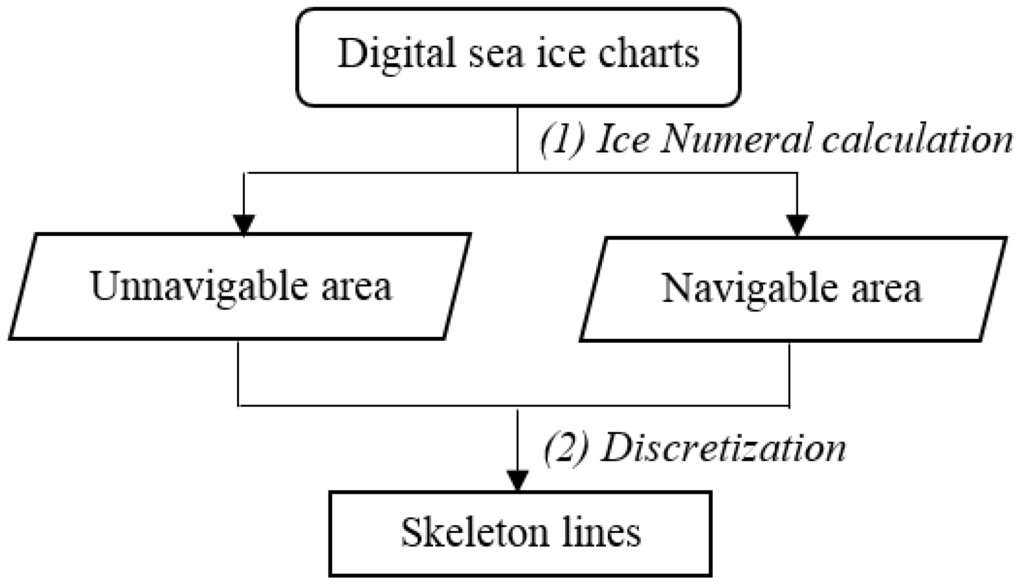
Figure 1.
A two-stage solution to automatic ice navigation.
2.2. Delineating Navigable Sea Area
Sea areas can be divided into two parts: navigable sea areas and unnavigable sea area, from navigation perspective. While both types of areas are constantly changing due to variation in ice coverage over time, the first part is continuous and the second part is consisted of numerous separated pieces. To determine whether or not it is safe to enter an ice regime, [2] introduced Ice Numeral (IN) method as the indicator and [23] proposed a GIS method to calculate IN. We follow the same method to delineate navigable sea areas from ice regimes. For the sake of convenience, we simply introduce the method [2,23] using artificial data. For more details, please refer to the above two papers.
Sea ice can be classified by its stage of development and concentration. Concentration is the “ratio expressed in tenths describing the area of the water surface covered by ice as a fraction of the whole area” [26]. An ice regime (colored polygons in Figure 2a) could consist of a mixture of ice types with varying concentrations and thicknesses [23] and can be digitally represented as egg code (Figure 2b) with “concentrations, stages of development (age) and form (floe size) of ice” in a simple oval form [26].
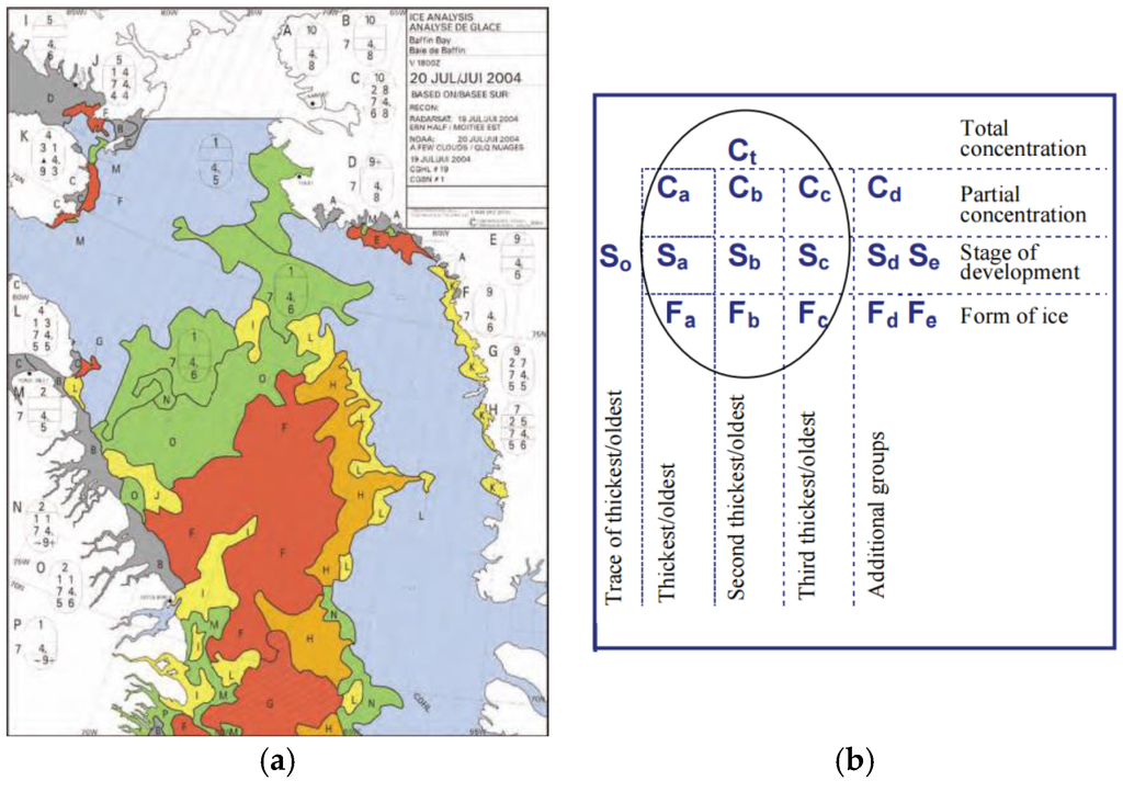
Figure 2.
The color-coded daily ice chart example (a) and Egg Code (b) of ice regime. The colored areas are ice regimes; Ca, Cb, and Cc and Fa, Fb, and Fc correspond to Sa, Sb, and Sc, respectively. (Source: [26], where two figures are directly cited without copyright issue).
Ice numeral (IN) was designed by [2] to measure the ability of a type of ship to navigate through this ice regime. IN can be calculated by using Equation (1):
where Ca is the concentration in tenths of ice type a, and IMa is the ice multiplier (IM) for ice type a, and the rest can be done in the same manner. IMs are used to indicate how much weight can be given to an ice type for a type of ship (see Table 1).
IN = (Ca * IMa) +(Cb * IMb) + … + (Cn * IMn)

Table 1.
Ice Multiplier (IM) based on ship types (Source: [27]).
If the ice numeral calculated for a type of ship is zero or positive, the ship can navigate through that ice regime. Conversely, if the ice numeral is negative, this type of ship cannot navigate through that ice regime unless an alternative plan such as using ice breaker to assist the ship is to be adopted. For example, suppose that an ice regime consists of 8/10ths total ice concentration, of which 1/10th is old ice and 7/10ths is thick first-year ice. While doing the calculation, remember to incorporate the 2/10ths open water [27]:
Type A ship: (1 × −4) + (7 × −1) + (2 × 2) = −7 (Negative regime)
CAC 4 ship: (1 × −3) + (7 × +1) + (2 × 2) = +8 (Positive regime)
The calculated INs reflect how they fluctuate for the same ice with structurally different ships. In the above example, Type A ship cannot navigate through the ice regime, while Type CAC4 ship can navigate it through safely. In this way, we are able to delineate navigable sea areas for different types of ships by using GIS vector-formatted digital ice charts.
2.3. Generating Voronoi Diagrams for Ship Route Planning
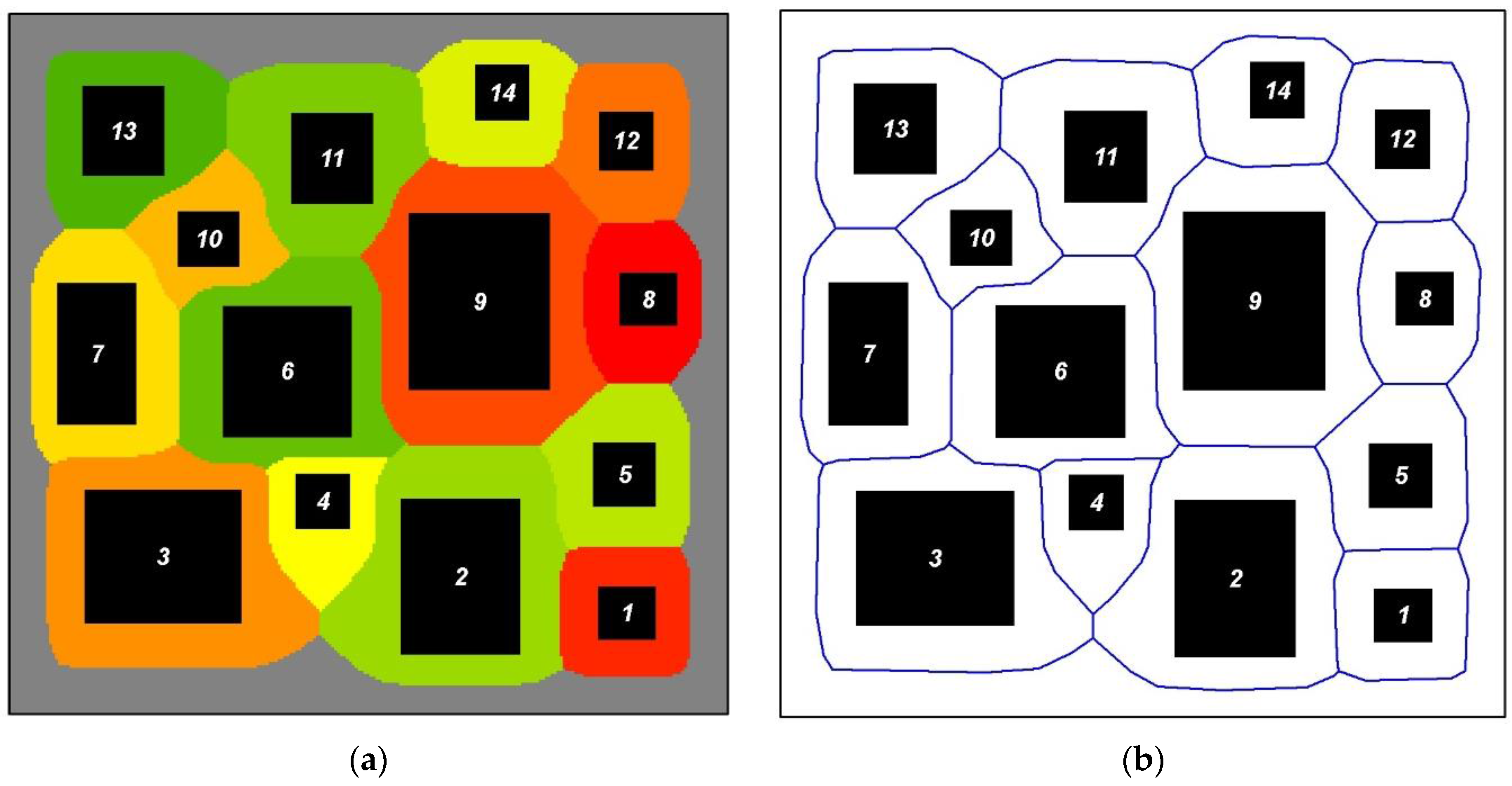
When navigating in the sea, ice navigators must be aware of where, what type and how much of ice regime is around them. Theoretically, ships can navigate at any location in positive regimes. However, to select the safest ship route, the best strategy is to keep them as far as possible from the negative regimes with high concentration [27]. In Figure 3, there are 14 artificial obstacles in black that are unnavigable sea areas, and the minimum bounding rectangle is used to describe their boundaries. We generate Voronoi Diagrams for these 14 obstacles, which are colored areas in Figure 3a. Based on the mathematical definition of a Voronoi Diagram, the distance between each point within a Voronoi Diagram and the obstacles is shorter than the distance between the point and any other obstacles. As a result, the boundary (blue lines in Figure 3b), which we call skeleton, of a Voronoi Diagram is the bisector of the space between any two obstacles, and any point on the boundary has the farthest distances to all the closest obstacles at the same time. Because of this, skeletons fully comply with the safest navigate principle in the sea.

Figure 3.
Voronoi Diagrams (colored regions) of 14 obstacles (black rectangles) on the left (a) and skeleton (boundaries of Voronoi Diagrams) in blue lines on the right (b).
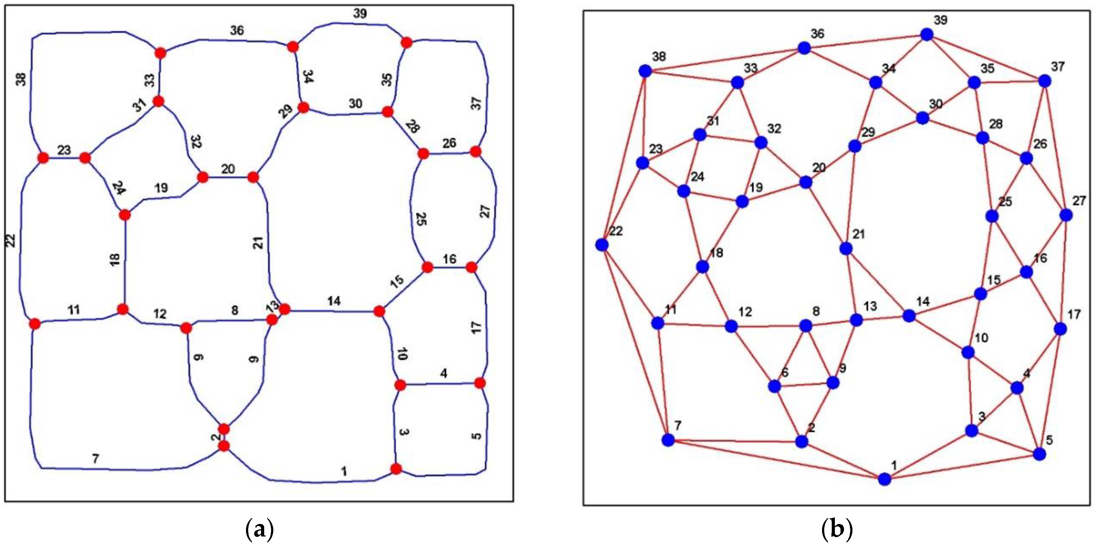
To this point, we have explained why it is safe to navigate along the skeletons of negative regimes in the sea. There are 39 skeletons and 26 junctions (blue lines and red points in Figure 4a) that are generated for the 14 unnavigable obstacles shown as black rectangles in Figure 3. These skeletons and junctions are a kind of road-network-like graph, and Figure 4b is the dual graph, of which blue points mean skeleton lines while red lines mean connections among them. Based on such a graph, we can apply any route planning algorithm (e.g., [27]) to automatically calculate ship routes between any pair of origin and destination in the sea.
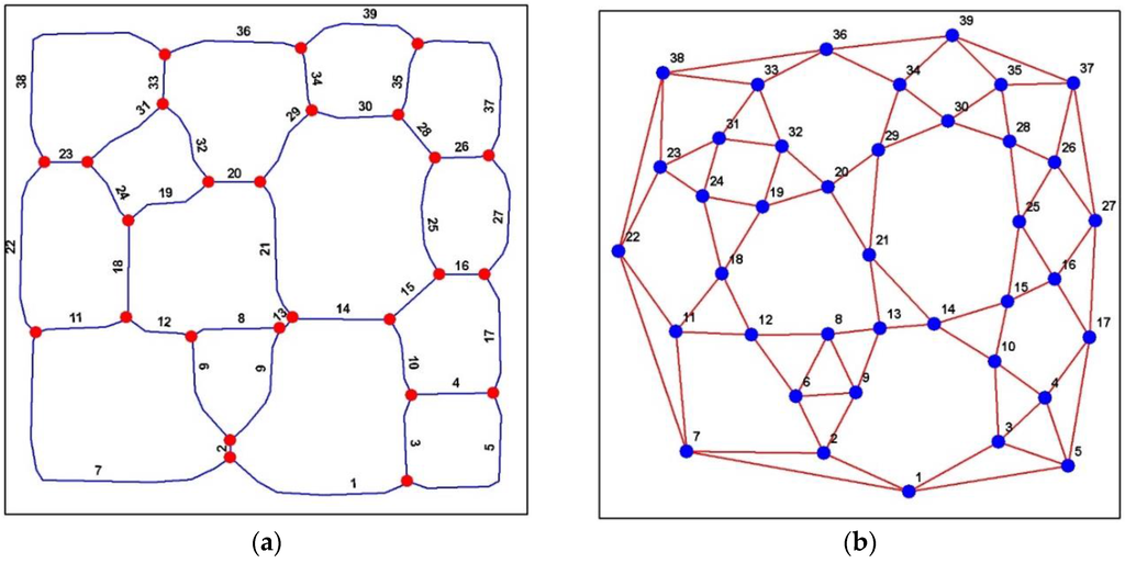
Figure 4.
Skeleton (39 blue lines) and junctions (26 red points) on the left (a) and its dual graph on the right (b): blue points means 39 skeleton lines and 78 red lines means the connections.
2.4. Isovist for Identifying Safe Navigable Areas
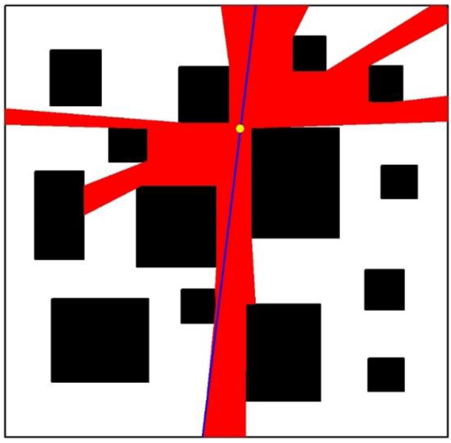
An Isovist is a visibility area from a single point of view in an open space. The concept of Isovist has been introduced into and useful for spatial analysis [28]. In navigable sea areas, an Isovist represents the safe navigable areas from current viewpoint. The integration of Isovist into ice navigation service would potentially be able to help navigator to identify such safe navigable areas in real time, given data availability. Figure 5 is an example of Isovist based on the artificial data described in Section 2.2.

Figure 5.
Isovist example in the artificial environment, where the black rectangles are the unnavigable areas, the yellow point is current position, the red area is the visibility area, and the blue line is the ridge, which is the longest line inside the visibility area.
3. Results and discussion
In this section, we formalize and implement the methods and algorithms described in Section 2 as a GIS package, namely NavSpace, which is shared online as an open source project for validation and extension, and which we hope to further attract contributions from related communities. A case study is further carried out by applying NavSpace to the digital vector-formatted sea ice charts produced by the Canadian Ice Service. For more details of the sea ice data, please refer to its official website [6].
3.1. Implementation and Experiments in Arctic Sea
We design and develop an open source Environmental Systems Research Institute (ESRI) ArcGIS extension, namely NavSpace, to help ship route planning in Arctic Sea. The development environment is Microsoft Visual Studio 2010 (VS2010) ASP.net using C# programming language, which is object-oriented and user-friendly developing tool for the Windows platform. We choose ArcObjects provided by ESRI ArcGIS to implement visualization and spatial analysis functions. The advantage of ESRI ArcObjects lies in its capability to provide visualization and spatial analysis interfaces that can be integrated into the NavSpace, which greatly reduces the time commitment in the development. Moreover, both Microsoft and ESRI ArcGIS are mainstream software packages that provide good continuity in terms of version update and maintainability throughout the life cycle of a software project.
The Arctic sea is selected as our study area (see Figure 6) because of two main reasons: (1) the availability of digital sea ice charts in this area; and (2) a sea ice project for the Canadian Ice Service Archive, namely CanICE, has developed a sea ice information database and web-based portal with novel, interactive knowledge discovery tools [11] in this area. Especially, a series of Google Maps-like sea ice web application programming interfaces (APIs) for JavaScript have been developed and an online web sandbox to facilitate debugging and sharing other types of ice web services have been provided [12]. Although the implementation and deployment of sea ice navigation service is targeted for general purpose in any sea ice areas, with the help of the open platform of CanICE, it would be easier to test, integrate and further popularize ice navigation service as part of the CanICE project.
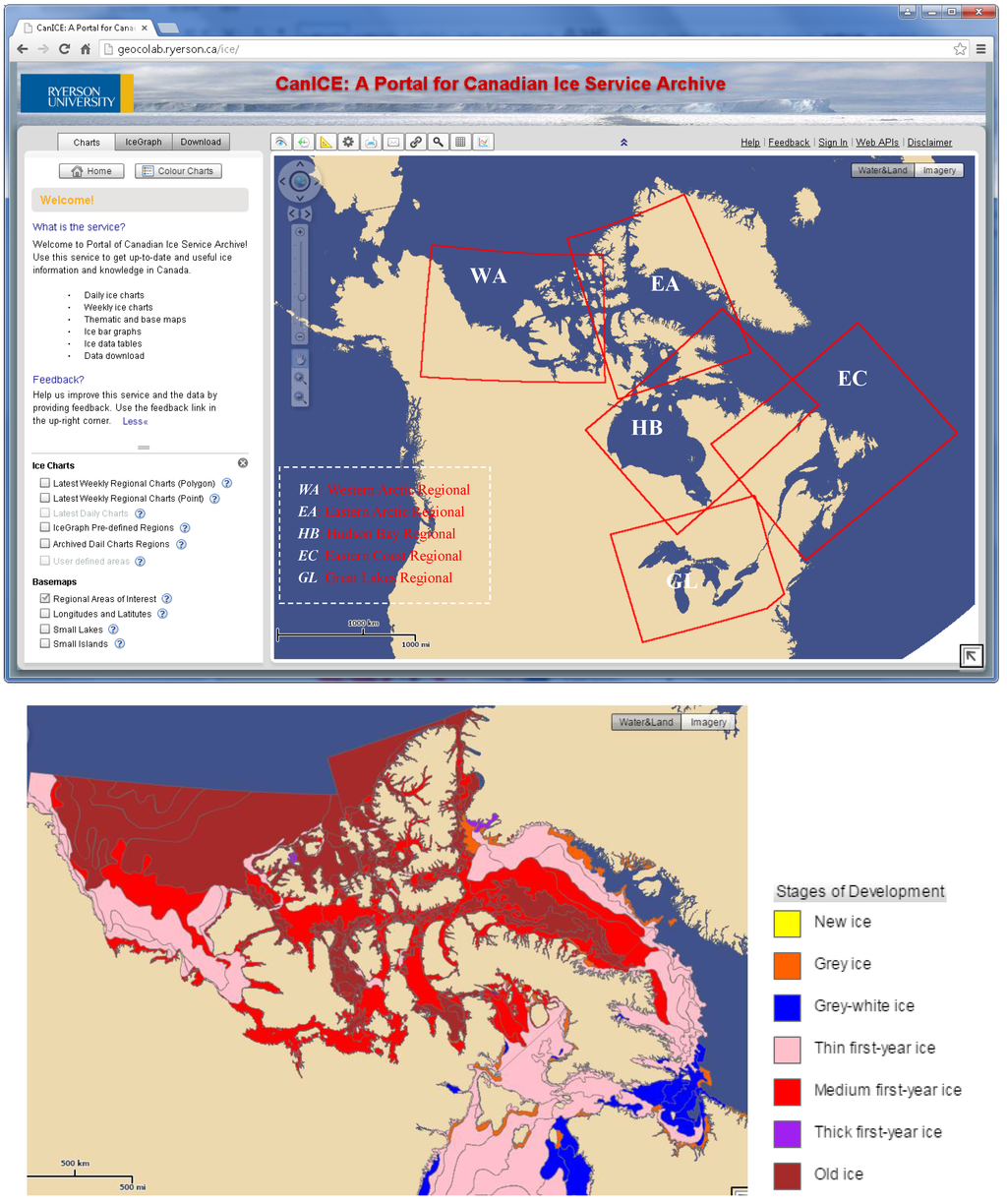
Figure 6.
Five regions of interest in the Arctic sea (upper part) where digital sea ice charts are available, and an example digital sea ice charts rendered by stages of development (lower part). (Source: captured from [29], where two figures are adapted from without copyright issue).
3.2. Generation of “Road-Network-Like Graph” in Arctic Sea
The Arctic sea is divided into five regions of interest (see the upper part in Figure 6), and we focus on the Western Arctic and Eastern Arctic Regions because there are many islands that increase the complexity of sea ice navigation. In the lower part of Figure 6, the visualized sea ice (colored by its stages of development) together with these islands makes it hard to manually plan route for different types of ships.
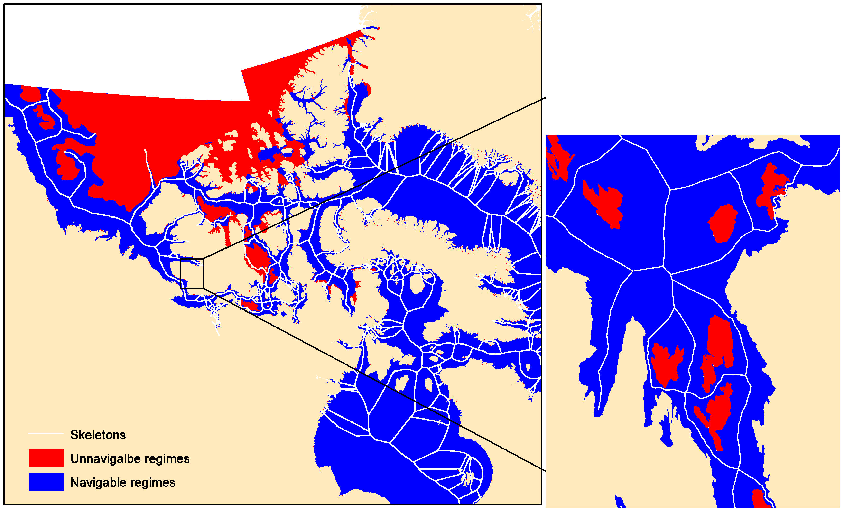
We download the digital sea ice charts on 2 February 2015 and convert it into ArcGIS-supported shape file format (the coordinate system is PS100) to carry out the case study in the Arctic sea. By applying the two-stage solution (see Figure 1) and using the developed GIS package NavSpace, firstly we calculate ice numeral (INs) for ship type CAC3 (refer to Table 1 in Section 2.1). The results are visualized in Figure 7, where the red is unnavigable ice regimes (i.e., with negative IN values) while the blue is navigable ice regimes (i.e., with positive IN values). Obviously, sometimes the islands are geographically connected with unnavigable regimes, which are spatially merged together to obtain obstacles when generating Voronoi Diagrams. The white lines in Figure 7 are the generated skeleton lines, which are used to build the “road-network-like graph” in the sea for automatic ship route planning. On the right is the detailed view of an area of interest in the black rectangle on the left.

Figure 7.
Navigable (or positive) regimes in blue, unnavigable (or negative) regimes in red and skeleton lines in white on 2 February 2015 for ship type CAC3.
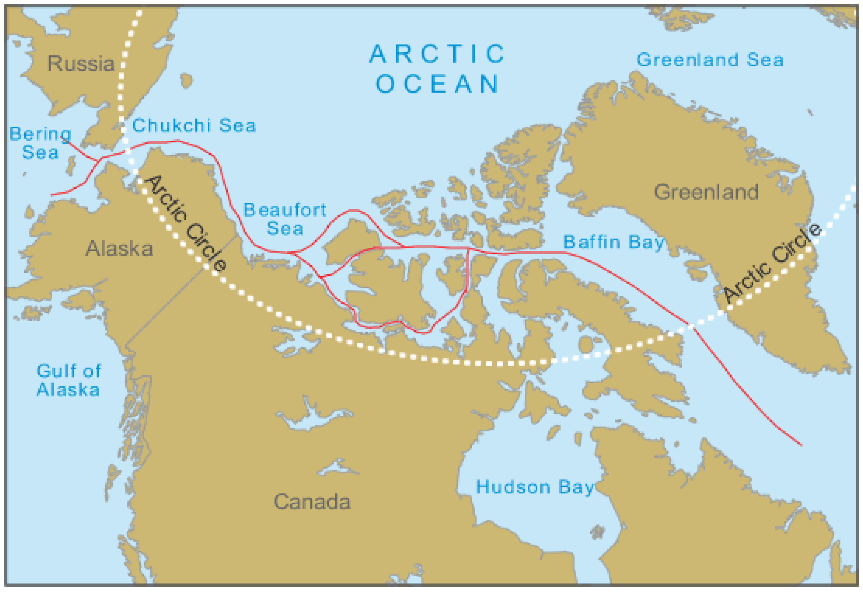
According to the methodology described in Section 2.2, we can build up a “road-network-like graph” based on the generated skeletons (white lines in Figure 7). Then we can apply any shortest path algorithms to the graph to calculate the shortest and safest routes for ship navigation. It means that the ship route will navigate along the skeletons. One question may arise here: Are there any real sea routes that also follow the skeleton method? In Figure 8, the Northwest Passage sea route that connects the Atlantic and Pacific Oceans through the Arctic Ocean is shown as the red lines. Although the Northwest Passage has been served as the recommended route for all types of ships without considering the variation of sea ice over time, visually we can see that it follows the sea ice navigation principle: keep as far as possible away from unnavigable regimes. Because of this, the Northwest Passage is consistent with the proposed method in this study. More importantly, the proposed method has the advantages in dealing with sea ice variation over time with the support of GIS techniques.
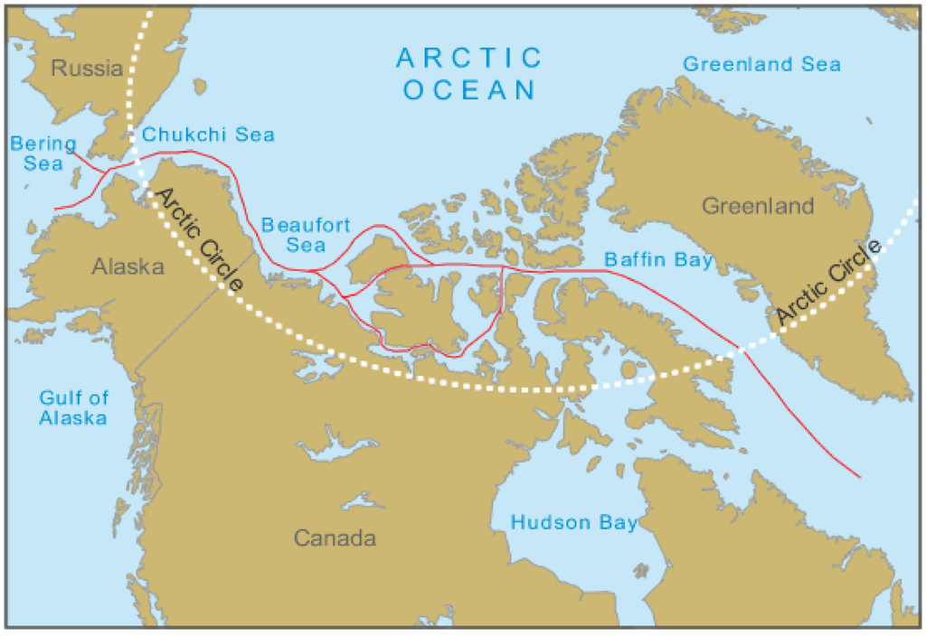
Figure 8.
Northwest Passage: red lines are possible ship routes (source: [30], where this figure is directly cited without copyright issue).
3.3. Automatic Ship Route Planning
An origin and destination pair O and D (two white triangles in Figure 9), respectively, is set up in the local area of interest. By applying the Dijkstra shortest path algorithm integrated in NavSpace to the “road-network-like graph” in the sea, we can get the shortest yet safest path (shown as the bold black line in Figure 9a), of which the total length is 84.4 kilometers. As mentioned previously, the shortest path is also the safest because such path also follows the safest navigation regulation, i.e., to keep as far as possible away from unnavigable regimes when navigating in the sea.
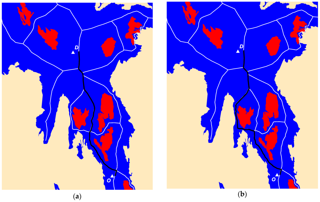
Figure 9.
The shortest and safest path (a) in black and the weighted shortest and safest path (b) in black between Origin and Destination pair for ship type CAC3.
Noticeably, according to [27], it is also important that the ships should navigate along the coastlines as much as possible in the sea. To solve this problem, a weighted shortest path algorithm is developed in NavSpace. In weighted shortest path algorithm, rather than using the geometric length of each skeleton, we use weight of each skeleton line to calculate shortest route. The weight is calculated in the following way: we simply calculate the closest distance between each skeleton line segment and coast line, and the weight to each skeleton line is just in inverse proportion to such normalized distance. It means that the closer the skeleton line is to coast lines, the higher the weight of the skeleton line segment has, and vice versa. After that, when we calculate the shortest path between OD pairs, we also obtain the weight of each possible path. To satisfy the above two navigation safety regulations, we can just select such a path that has the highest weight and its length is also close to the shortest path. It is a kind of balance between travel distance and safety. For example, on the right side of Figure 9b, the length of the path (black bold line) between the OD pair is 93.5 kilometers. It is a bit longer than the one in Figure 9a, but has the higher weight, which means that it best fits the two navigation rules: closer to cost lines and having higher weight.
3.4. Isovist: Automatic Identification of Navigable Areas
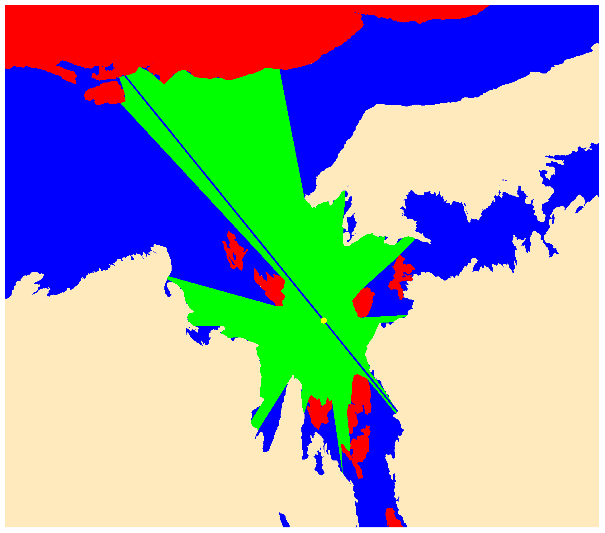
In Section 3.2 and Section 3.3, we demonstrated how to build a “road-network-like graph” in the sea and finally apply the Dijkstra shortest path and weighted shortest path algorithms to the graph to calculate the shortest and safest route. However, in some situations, navigators need be aware of the navigable areas from current location of the ship to guide ship navigation, e.g., fishing ship needs to randomly navigate in some sea areas. Figure 10 is the example of visual analysis in the Arctic sea.

Figure 10.
The navigable/visible area in green generated using Isovist for Type CAC3 ship, where the yellow point is the current position.
The yellow point in Figure 10 is the current ship location, and the green polygon area is the visible or navigable area, where we can apply Isovist as described in Section 2.3. We implement the Isovist algorithm as a spatial analysis tool and integrate it as part of NavSpace to support sea ice navigation. It should be noted that, though the Isovist tool is developed to identify the navigable or visible areas when navigating in the sea, based on the boundary of the visibility area, we are able to know more information of the reachable area, e.g., whether it is near the coastline or if there is any kind of ice. This tool can help navigator make quick decisions in some emergency situations.
It should also be noted that, though the generation of shortest and safest path as well as the Isovist analysis is automatic and in real time, the data processing is semi-automatic and not in real time. For example, the generation of skeleton lines takes around ten minutes using a mainstream desktop computer with typical configuration for each type of ship using weekly ice charts. Once the data processing is done, the initialization of the “road-network-like graph” takes around two minutes. The Canadian Ice Service updates the ice data on a daily or weekly basis, therefore, there is enough time to process ice data to support sea ice navigation. In the future, in the case that sea ice data update in real-time, a dynamic Voronoi Diagram method should be developed to generate real-time sea ice navigation skeletons, which means instead of updating the whole Voronoi Diagrams, only the changed sea ice areas will be reconstructed.
4. Conclusions
In this study, we make several important new contributions to the literature on automatic ice navigation support service in a time-geographic context. From a methodological perspective, we formalize algorithms for automatic ship routing and visual analysis based on ice numeral, and develop an analytical GIS package. It is available as an open source tool (link available for downloading at [31]) for validation and extension. This easy-to-use ArcGIS tool is also useful for interested readers in relevant research, for example, indoor navigation study. The methodology is demonstrated using the Canadian Ice Service Archive data.
A number of future studies can be conducted. We have demonstrated the capacity to automatically navigate in the sea in real time and implemented it in an open source GIS package. An online version with a real-time dashboard is to be designed for sea ice navigation agency by integrating live data feeds and other types of real-time sea events for managing operations, which will offer researchers new insights in real-time sea ice navigation support. As for the validation of the methods and results, especially using real ship routes, it will be our future work as long as we have access to real navigation data.
Acknowledgments
This research has been funded in part by the Beaufort Regional Environmental Assessment (BREA) Initiative, which was funded by the Aboriginal Affairs and Northern Development Canada, and by the National Science and Engineering Research Council of Canada (Grant #RGPIN/250346-2011). The authors also wish to thank the Canadian Ice Service Archive for the ice data used in this study and its staff for their comments received during CanICE project execution.
Author Contributions
Xintao Liu, Shahram Sattar and Songnian Li conceived of and designed the study. Xintao Liu and Shahram Sattar analyzed the data and performed the experiments. Xintao Liu, Shahram Sattar and Songnian Li wrote and revised the paper together. All authors have read and approved the final manuscript.
Conflicts of Interest
The authors declare no conflict of interest.
References
- Snider, D. Ice navigation in the Northwest Passage. In Proceedings of the Ocean Innovation 2005, Rimouski, QC, Canada; Quebec, QC, Canada, 23 October 2005.
- Transport Canada. Arctic Ice Regime Shipping System (AIRSS): User Assistance Package for the Implementation of Canada’s Arctic Ice Regime Shipping System (AIRSS); Transport Canada: Ottawa, ON, Canada, 1998. [Google Scholar]
- Bell, T.; Briggs, R.; Bachmayer, R.; Li, S. Augmenting Inuit knowledge for safe sea-ice travel—The SmartICE information system. In Oceans-St. John's; IEEE: New York, NY, USA, 2014; pp. 1–9. [Google Scholar]
- Transportation Safety Board of Canada. Available online: http://www.tsb.gc.ca/eng/stats/marine/2012/ss12.asp (accessed on 17 January 2016).
- Barry, R. The sea ice database. In The Geophysics of Sea Ice; Untersteiner, N., Ed.; Plenum Press: New York, NY, USA, 1986; pp. 1099–1134. [Google Scholar]
- Drinkwater, K.F. Climatic Data for the Northwest Atlantic: A Sea Ice Database for the Gulf of St. Lawrence and the Scotian Shelf; Fisheries & Oceans Canada, Maritimes Region, Ocean Sciences Division, Bedford Institute of Oceanography: Halifax, NS, Canada, 1999. [Google Scholar]
- Knight, R.W. Introduction to a new sea-ice database. Ann. Glaciol. 1984, 5, 81–84. [Google Scholar]
- Lenormand, F.; Duguay, C.R.; Gauthier, R. Development of a historical ice database for the study of climate change in Canada. Hydrol. Process. 2002, 16, 3707–3722. [Google Scholar] [CrossRef]
- Liu, X.; Li, S. Towards a spatiotemporal database model for Canadian ice service portal. In Proceedings of Canadian Institute of Geomatics Annual Conference and the 2013 International Conference on Earth Observation for Global Changes (EOGC’2013), Toronto, ON, Canada, 5–7 June 2013.
- Eicken, H.; Lovecraft, A.L.; Druckenmiller, M.L. Sea-ice system services: a framework to help identify and meet information needs relevant for Arctic observing networks. Arctic 2009, 62, 119–136. [Google Scholar] [CrossRef]
- Li, S.; Xiong, C.; Ou, Z. A Web GIS for sea ice information and an ice service archive. Trans. GIS 2011, 15, 189–211. [Google Scholar] [CrossRef]
- Liu, X.; Li, S.; Huang, W.; Gong, J. Designing sea ice web APIs for ice information services. Earth Sci. Inform. 2015, 8, 483–497. [Google Scholar] [CrossRef]
- Ou, Z. An integrated spatial information system for ice service. In Proceedings of the 20th ISPRS Congress, Istanbul, Turkey, 12–23 July 2004; pp. 12–23.
- Arctic and Antarctic Research Institute (AARI). Available online: http://www.aari.nw.ru/index_en.html (accessed on 17 January 2016).
- Canadian Ice Service (CIS), Environment Canada. Available online: https://www.ec.gc.ca/glaces-ice (accessed on 17 January 2016).
- Finnish Meteorological Institute (FMI). Available online: http://en.ilmatieteenlaitos.fi/ (accessed on 17 January 2016).
- NASA. An Overview of EOSDIS. Available online: https://earthdata.nasa.gov/about-eosdis (accessed on 17 January 2016).
- National Ice Center Institute (NIC). Available online: http://www.natice.noaa.gov (accessed on 17 January 2016).
- Polar Data Catalogue (PDC). Available online: https://www.polardata.ca/ (accessed on 17 January 2016).
- Chen, X.; Liu, X.; Li, S.; Chow, A. A comparative study on three EOF analysis techniques using decades of Arctic sea-ice concentration data. J. Cent. South Univ. 2015, 22, 2681–2690. [Google Scholar] [CrossRef]
- Rayner, N.A.; Parker, D.E.; Horton, E.B.; Folland, C.K.; Alexander, L.V.; Rowell, D.P.; Kent, E.C.; Kaplan, A. Global analyses of sea surface temperature, sea ice, and night marine air temperature since the late nineteenth century. J. Geophys. Res.: Atmos. 2003, 108. [Google Scholar] [CrossRef]
- Rothrock, D.A.; Thomas, D.R.; Thorndke, A.S. Principal component analysis of satellite passive microwave data over sea ice. J. Geophys. Res.: Oceans 1988, 93, 2321–2332. [Google Scholar] [CrossRef]
- Howell, S.E.; Yackel, J.J. A vessel transit assessment of sea ice variability in the Western Arctic, 1969–2002: Implications for ship navigation. Can. J. Remote. Sens. 2004, 30, 205–215. [Google Scholar] [CrossRef]
- Khon, V.C.; Mokhov, I. Arctic climate changes and possible conditions of arctic navigation in the 21st century. Izvestiya. Atmos. Ocean. Phys. 2010, 46, 14–20. [Google Scholar] [CrossRef]
- MaxSea, Marine Navigation Software. Available online: http://www.maxsea.com (accessed on 17 January 2016).
- Canadian Ice Service (CIS). Manual of Standard Procedures for Observing and Reporting Ice Condition; Canadian Ice Service, Environment Canada: Ottawa, ON, Canada, 2005. [Google Scholar]
- Canadian Coast Guard (2012). Ice Navigation in Canadian Waters; Icebreaking Program, Maritime Services, Canadian Coast Guard, Fisheries and Oceans Canada: Ottawa, ON, Canada, 2012. [Google Scholar]
- Turner, A.; Penn, A. Making isovists syntactic: Isovist integration analysis. In Proceeding of the 2nd International Symposium on Space Syntax, Brasilia, Brazil, 29 March 1999.
- CanICE. Available online: http://geocolab.ryerson.ca/ice (accessed on 10 March 2016).
- Geology. Available online: http://geology.com (accessed on 10 March 2016).
- NavSpace. Available online: https://github.com/xintao/NavSpace (accessed on 10 March 2016).


© 2016 by the authors; licensee MDPI, Basel, Switzerland. This article is an open access article distributed under the terms and conditions of the Creative Commons by Attribution (CC-BY) license (http://creativecommons.org/licenses/by/4.0/).