Method for Mapping Rice Fields in Complex Landscape Areas Based on Pre-Trained Convolutional Neural Network from HJ-1 A/B Data

Abstract

Accurate and timely information about rice planting areas is essential for crop yield estimation, global climate change and agricultural resource management. In this study, we present a novel pixel-level classification approach that uses convolutional neural network (CNN) model to extract the features of enhanced vegetation index (EVI) time series curve for classification. The goal is to explore the practicability of deep learning techniques for rice recognition in complex landscape regions, where rice is easily confused with the surroundings, by using mid-resolution remote sensing images. A transfer learning strategy is utilized to fine tune a pre-trained CNN model and obtain the temporal features of the EVI curve. Support vector machine (SVM), a traditional machine learning approach, is also implemented in the experiment. Finally, we evaluate the accuracy of the two models. Results show that our model performs better than SVM, with the overall accuracies being 93.60% and 91.05%, respectively. Therefore, this technique is appropriate for estimating rice planting areas in southern China on the basis of a pre-trained CNN model by using time series data. And more opportunity and potential can be found for crop classification by remote sensing and deep learning technique in the future study.

1. Introduction

Rice spatial distribution and area information have great significance for yield prediction, greenhouse gas emission and human food security. Rice provides a stable source of energy for more than half of the world’s population, most especially Asians [1,2]. However, surveys indicate that agricultural areas were on a decline in the period of 1994–2014 and that rice planting fields only occupy approximately 11% of global arable regions [3,4]. As global warming intensifies, rice plays an increasingly important role that cannot be neglected because it can generate considerable amounts of methane gas, which accounts for approximately 5–19% of the global emission to the atmosphere [5,6]. Food security, which is closely related to life security, has recently become the focus worldwide [7]. A comprehensive understanding of rice fields could aid the government’s decision making for resource management [8]. Hence, precise information about rice planting areas is highly critical nowadays.

Unlike the field investigation in the past, remote sensing represents an important approach to Earth observation and is thus becoming widely popular in crop monitoring because of its large coverage, real-time capabilities and low costs [9]. The existing literature proposes several approaches for estimating rice planting areas based on remote sensing. These approaches are grouped into three types. First, as a response to survival circumstances, phenological features could well reflect regular changes in different plants, which are captured by various vegetation indexes (VIs) in practice [10,11,12]. Many studies have been conducted on the basis of the temporal curves of VIs, such as the normalized difference vegetation index (NDVI), enhanced vegetation index (EVI) and land surface water index (LSWI), given the unique component of rice planting areas, which is a mixture of soil, water and plants during key phenological stages (transplanting and early growing period) [13,14]. Different thresholds are also set to distinguish rice areas from other land types. For example, Chen [15] mapped rice fields in the western regions of Guangdong province by analyzing the characteristics of the temporal NDVI derived from the China environment satellite data. Thereafter, a novel VI known as the two-band enhanced vegetation index (EVI2) emerged, achieving high consistencies across sensors because it merely involves two bands without a blue one [16]. Wang [17] provided the threshold referring signatures of the temporal profile of EVI2 to identify single-cropped rice in a fragmented area. In further studies, multiple VIs (NDVI coupled with EVI, LSWI, or others) were utilized to determine the threshold for estimating rice planting areas [14,18,19,20,21]. Second, several algorithms have been designed on temporal VI profiles. Previous studies developed a dynamic time warping (DTW) method for similarity-based time series data matching, which is commonly applied in disturbance classification, speech recognition and other time series categories [22,23,24]. Guan [25] identified rice growth areas with the NDVI-based DTW method. And NDVI time series profiles for each pixel were built and the DTW distance with the standard rice growth NDVI profile was calculated for similarity comparison. Then rice areas could be extracted by setting thresholds. However, this approach obtains unsatisfactory outcomes because it neglects that different time intervals exist between different similar point pairs when finding the best alignment between two time series [26]. Therefore, a substantial number of improved algorithms have been proposed in other research and they perform better than the original DTW, such as the Time Weighted Dynamic Time Warping (TWDTW) algorithm which introduced a time constraint accounting for seasonality of land types [27,28]. Finally, considerable classification approaches have been used in the existing literature. On the one hand, traditional models were mostly built on the basis of the statistical characteristics of images and they include the maximum likelihood classifier (MLC) and iterative self-organizing data analysis technique (ISODATA) [29,30,31]. However, these models are turned out to be a lower robust due to spectral variability [32]. On the other hand, following the development of machine learning, several high automation methods, such as neural network, SVM, decision tree and random forest, have been greatly utilized for remote sensing classification [33,34,35]. However, the aforementioned models have a shallow structure, which fail to extract deep signatures of various land types in satellite images. Recently, a power image processing technique, that is, deep learning, has emerged. With deep networks, it can extract numerous features in hierarchical structures; hence, numerous deep networks have been built in the field of remote sensing [36]. Among them, CNN is the most effective in extracting deep features by convolution process and achieving an outstanding performance [37,38,39,40]. However, CNN-based classification methods in remote sensing mainly rely on high-resolution or hyperspectral images with high cost and poor efficiency. Hence, new attempts must be made in the recognition of rice areas from mid-resolution data based on deep learning models.

Generally, the difficulties in rice field mapping accurately are strongly correlated with rice spatial distribution, tillage mode and growing conditions. In southern China, rice is widely cultivated in areas where croplands are highly fragmented with little patches and plant structure is highly complex, leading to errors in distinguishing rice areas from surrounding land types. The current study seeks to determine whether we can use temporal VI features to obtain precise information about rice planting areas with the aid of deep learning. The approaches based on temporal VI determine the selection of high temporal resolution satellite data. Moderate resolution imaging spectroradiometer (MODIS) images are commonly used in previous research. However, despite their high temporal resolution, MODIS images are not appropriate for our study because they may cause a mix-pixel problem due to low spatial resolution. Accordingly, retrieving satellite data calls for appropriate spatial and higher temporal resolution. In comparison with Landsat information with a 16-day revisit cycle, HJ-1 A/B satellite data, which exhibit a 30 m spatial resolution and a four-day revisit cycle (unite for two days), bring a new direction for time series development. As we mentioned previously, CNN is significant in estimating rice fields and effective in extracting deep features. However, the number of available samples from remote sensing images is limited, making it difficult to support the training step. Transfer learning occurs with sharing knowledge from one or more source tasks and then applying such knowledge to a similar target domain [41]. Hence, we are interested in the use of the CNN model for extracting features of temporal VI through introducing the transfer learning method instead of training from scratch. For comparison, the SVM model is also used in experiment. SVM is a nonparametric classifier with a shallow structure that transforms a linear inseparable problem from a low dimensional space into a high dimensional feature space via a nonlinear mapping algorithm to make such problem linearly separable [42].

Considering the necessity and challenges of mapping paddy rice fields with complex landscapes in southern China, we aim to explore the feasibility of using the CNN deep model for accurate rice field mapping on the basis of VI time series images. This study ultimately provides a pixel- and deep temporal feature-based model for rice area extraction. Meanwhile, the SVM model is also used for comparison.

2. Materials and Data Processing

2.1. Study Area

Zhuzhou City is situated in the east of Hunan Province, China, expanding from 26°03′05″ to 28°01′07″ E and 112°57′30″ to 114°07′15″ N (World Geodetic System-1984 (WGS-84) Coordinate System) and is adjacent to Xiangjiang River (Figure 1). The city is part of the subtropical monsoon zone with sufficient sunlight and warm and humid climate. Paddy rice cultivation is abundant in this city due to the annual average temperature of 16–18 °C and precipitation of 1500 mm. The city is also a famous commodity grain base in China. Additionally, Zhuzhou City belongs to typical hilly landforms, hence the patchiness and fragmentation of its cropland. Furthermore, the complex planting structure in this region heightens the difficulty in accurately estimating rice fields on remote sensing images. Thus, Zhuzhou is appropriate for our study.

2.2. Data Collection and Pre-Processing

2.2.1. Satellite Data

Eight HJ-1 A/B images from 13 May to 3 November 2017 were collected in our work to generate EVI datasets for machine learning and classification.

Table 1. Acquisition of remote sensing data.

No.	Satellite	Sensor	Spatial Resolution (m)	Acquisition Date
1	HJ1B	CCD1	30	13 May 2017
2	HJ1B	CCD2	30	29 May 2017
3	HJ1A	CCD2	30	22 July 2017
4	HJ1A	CCD2	30	26 July 2017
5	HJ1B	CCD2	30	20 August 2017
6	HJ1A	CCD1	30	25 August 2017
7	HJ1B	CCD2	30	18 September 2017
8	HJ1A	CCD2	30	3 November 2017

summarizes the concrete acquisition date of these images. Among them, there are two images in May (13 May and 29 May), two images in July (22 July and 26 July), two images in August (20 August and 25 August), one image in September (18 September) and one image in November (3 November). All of the images were downloaded freely from the China Center for Resources Satellite Data and Application (http://www.cresda.com/CN/). The major parameters of the two satellites are presented in

Table 2. Major load parameters of HJ-1A/B satellites.

Platform	Payload	Channel	Spectral Range (μm)	Spatial Resolution (m)	Detection Width (km)	Revisit Cycle (day)
HJ-1A	CCD	1	0.43–0.52	30	360 (single), 700 (double)	4
		2	0.52–0.60
		3	0.63–0.69
		4	0.76–0.90
	HIS	−	0.45–0.95	100	50	4
HJ-1B	CCD	1	0.43–0.52	30	360 (single), 700 (double)	4
		2	0.52–0.60
		3	0.63–0.69
		4	0.76–0.90
	IRS	5	0.75–1.10	150	720	4
		6	1.55–1.75
		7	3.50–3.90
		8	10.5–12.5	300

. Two charge coupled device (CCD) sensors were loaded with 30 m spatial resolution, 360 km detection width and four-day temporal resolution. These sensors were also identical in the range of multispectral bands, which comprised four channels, that is, band 1 (blue): 0.43–0.52 μm, band 2 (green): 0.52–0.60 μm, band 3 (red): 0.63–0.69 μm and band 4 (near infrared): 0.76–0.90 μm.

All acquired images needed to be processed prior to use in ENVI5.2 image processing software (Exelis VIS, White Plains, NY, USA). The processing mainly covered the following five aspects. First, absolute radiometric calibration was performed for each band of the image according to the coefficient and formula of radiometric calibration that was provided by the China Center for Resources Satellite Data and Application and then stacked together for later use. Second, we obtained the spectral response curve data from the China Center for Resources Satellite Data to produce four spectral response functions and converted the image format to prepare for atmospheric correction. Third, we conducted the atmosphere correction through the FLAASH module (Spectral Sciences Inc. & U.S. Air Force Research Laboratory). Fourth, automatic registration was completed among CCD images to eliminate the errors of different sensors, with the root mean square (RME) error was less than one pixel. Finally, the images were uniformly re-projected to the Universal Transverse Mercator (UTM)-WGS84 system.

2.2.2. Ancillary Datasets

The ground-truth data, together with observation points from Google Earth, were used in this study to promote classification and verification. There were 3577 points for result verification in total. In field surveys, 419 points were visited and every land use patch covered more than 900 square meters. Then position that was located by a Global Position System (GPS) device and the corresponding land type of each site were recorded. Other points were selected from Google Earth randomly. All these points were stored to a raster dataset with a TIFF format and 30 m spatial resolution. This dataset can be regarded as reference data for accuracy assessment.

3. Methodology

A novel idea based on deep learning was proposed in this study to accurately estimate paddy rice areas in southern China. The workflow of our approach is shown in Figure 2. On the basis of EVI time series data, we applied the SVM model and CNN model to proceed classification, respectively. The CNN model was built by pre-trained method and the features of EVI time series curves (shape, amplitude and abstract features) could be extracted to assist classification. Then a comparative analysis on accuracy assessment between two results were completed. The concrete procedures are follows. (1) We calculated the VI of multitemporal satellite data and then reconstructed the time series curve as input. (2) A deep learning model for classification was developed on the basis of the framework of the Convolutional Architecture for Fast Feature Embedding [43], which introduced the strategy of transfer learning. (3) Model training and validation were conducted by selecting different samples. (4) For contrast, SVM and deep learning model were used for classification, separately.

3.1. Construction of EVI Time Series

Extensive research has suggested that VIs can be used to objectively reflect plant growth states with evident seasonal characteristics, periodicity and difference [19,44]. Thus, selecting a proper index for our study was critical. NDVI, one of the most popular VIs, was successfully used to crop monitoring [45,46]. However, saturation tends to occur in some regions with dense vegetation coverage, thereby limiting its further application. As an improved VI, EVI has attracted increasing attention given the interference of environmental factors and soil background. This index compensates for the saturation problem of NDVI and shows a high sensitivity to vegetation changes; hence, we chose this index instead of NDVI to detect different land types [33]. The EVI computational formula is given as follows:

$$\mathrm{EVI}=2.5\times \frac{{\rho }_{NIR}-{\rho }_{RED}}{{\rho }_{NIR}+6.0\times {\rho }_{RED}-7.5\times {\rho }_{BLUE}+1.0}$$

(1)

where ${\rho }_{NIR}$, ${\rho }_{RED}$ and ${\rho }_{BLUE}$ correspond to the reflectances of near- infrared, red and blue bands, respectively.

Despite the rigorous pre-processing operations conducted initially, it is clear that clouds, aerosols and other external factors (like shadow and snows) are going to appear in VIs [47,48]. Thus, a filtering algorithm is necessary to minimize noises in the next step. At present, three primary filtering algorithms are commonly used: double logistic model functions, asymmetric Gaussian model functions and Savitzky-Golay filtering method. In the current study, we chose the last to smoothen the EVI time series. The Savitzky-Golay method implements local polynomial fitting on time series to generate the filter value of each point; the major feature of it is to keep invariance of shape and width while removing noises [49]. Furthermore, interpolation and polynomial fitting procedures were introduced to obtain the daily EVI value. We illustrate the EVI time series of rice in Figure 3.

3.2. Extraction of Different Phenological Patterns

On the basis of the dense stack of satellite data, every land type has its own phenological sequence pattern corresponding to specific VI curves; this pattern could be introduced into crop classification with certain characteristics [28,50]. Therefore, we divide the study area into four major land types; water, forest, rice and others (like bare land, building and abandoned cropland). The unique characteristics of land types are expected to assist image classification. Therefore, it is extremely essential to learn more about the characteristics of EVI time series curves, which accounts for the phenological sequence patterns of objects. The typical EVI time series curves of four land types are illustrated in Figure 4.

3.3. Establishment of Classification Model Based on Deep Temporal Features

3.3.1. Architecture of CNN

With the advantages of local connections, shared weights, pooling and multiple layers, CNN, a famous feed-forward network, was chosen as the main framework of our proposed model, which consists of a number of neurons with learnable weights and biases [37,51]. We developed a model based on LeNet-5 (Yann LeCun), which has been perceived as the basic prototype of existing CNNs. We provided the model with a distinct architecture (Figure 5), including input, convolutional, pooling, fully connected and output layers, to improve our understanding of CNN.

Information is initially inputted into the network through the input layer for use in a later process. Next is the convolutional layer, which is the core module of the entire network and plays a significant role in feature extraction through convolution. There have multiple convolutional planes consist of numerous neurons. Each neuron is locally connected to the former layer by convolutional kernels, which simply dictate the feature extraction procedure. Then, a rectified linear unit (ReLU), a non-linear activation function, is introduced to add nonlinear ability [52]. We utilized various convolutional kernels convolved with the input to obtain different features. Although indefinite initially, these kernels were adjusted by frequent training.

Pooling, which is linked to the convolutional layer alternately, is calculated by down sampling to realize feature dimension reduction and that is why we also call it the down sampling layer. This layer mainly contributes to the reduction of the number of connections among neurons, which not only accelerates the computation but also helps to enhance robustness. The typical pooling algorithms are the max pooling and the average pooling [53]. Generally, the pooling layer is regarded as the secondary layer of feature extraction and is as important as the convolution layer.

The fully connected layer is aimed at implementing classification on the basis of locally separable features acquired from previous layers. Each neuron is fully linked to all neurons on the upper layer. The last layer is commonly considered as the output, where softmax logistic regression follows for classification task.

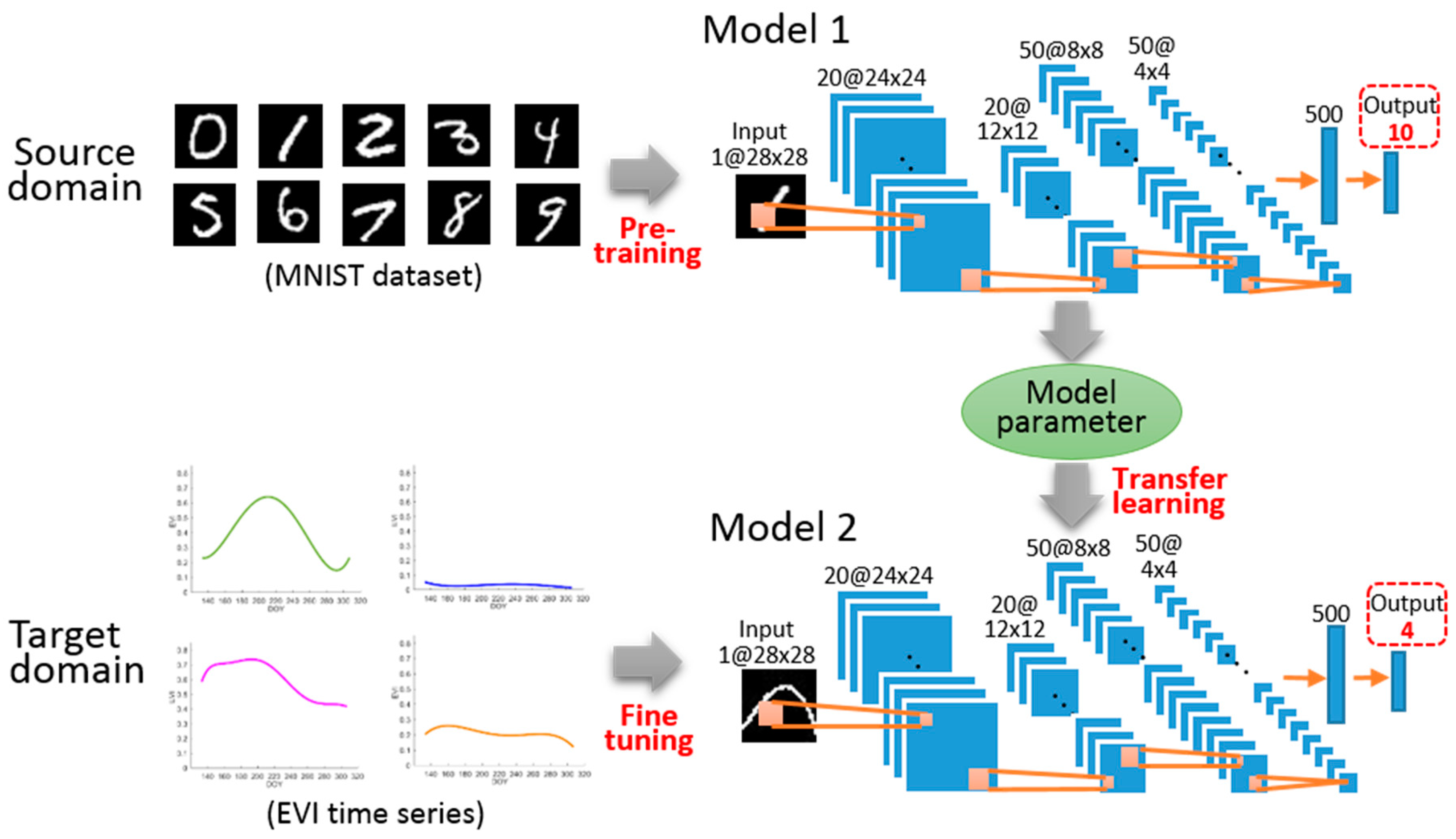
3.3.2. Strategy of Transfer Learning

In order to solve the problem about insufficient samples from remote sensing data, transfer learning, which can transfer previously knowledge to a new task, was introduced in our work. On the basis of the content that was transferred, the methods of transfer learning were divided into four categories; instance-based transfer learning, feature-based transfer learning, parameter-based transfer learning and relational-based transfer learning [41]. We used the parameter-based transfer learning that the model parameters were shared between target domain and source domain. In other words, the model, which was trained by using a large amount of data from source domain, was applied to target domain in which the model could be trained by less data. Therefore, the network could assimilate generic features to promote its application in small database [54].

In the experiment, the implementation of transfer learning was illustrated in Figure 6. First, we set up a pre-trained model (Model 1) by using the Modified National Institute of Standards and Technology (MNIST) database (http://yann.lecun.com/exdb/mnist/). The datasets consist of handwritten numerals from high school students and staff of the Census Bureau. Specifically, the datasets comprise 50,000 training samples and 10,000 testing samples, which are all in grayscale and normalized into 28 × 28 pixels. More significantly, different handwritten numerals were mainly distinguished by the shape of lines, which is similar to the EVI time series curve in our study. Subsequently, parameters of Model 1 were stored as an individual file which was transferred into Model 2. Ultimately, we conducted the fine tuning process by using EVI time series to determine the final CNN model.

There were 1893 samples for deep learning, which were collected randomly by visual interpretation and were sorted into training samples and testing samples according to the proportion of 2:1. And these samples must be normalized uniformly before model training. As mentioned above, it is essential to help the pre-trained CNN model reach an optimal state as much as possible by adjusting several training parameters. Here, we mainly discuss the effects of two types of parameters, that is, batch size and learning rate, on model performance. Batch size is briefly defined as the numbers of samples for each training. Commonly, a large batch size equates to a precise descent direction within a reasonable scope, as well as a slight oscillation. By contrast, a small batch size may introduce randomness and poor convergence. Therefore, a proper batch size should be set in relation to the sample scale. We adopted 100, 64 and 32 as batch sizes in the current work. Learning rate, another important factor, is a parameter for adjusting gradient descent steps in a network. It basically depends on the speed of parameters in reaching their best values. In other words, an excessively high learning rate updates parameters rapidly, causing the network to easily converge into a local optimum. Conversely, an extremely low value reduces the efficiency and leads to a slow convergence. Thus, there is no doubt that setting up a proper learning rate is extremely necessary. We set the values of 0.1, 0.01 and 0.001 to explore the impacts of different learning rates on the results.

4. Results and Accuracy Assessment

4.1. Characteristics of EVI Time Series

From Figure 4, it can be seen that the shape, tendency and other aspects of the different temporal curves show obvious variances. First, rice fields are extremely unique because they are partially covered with a mixture of soil, water and rice seedlings during the transplanting and early growth periods [13]. Meanwhile, a low value is observed in the EVI curve. In the tilling and jointing stages, the roots and leaves develop rapidly and the EVI value increases sharply to a peak beyond 0.6. According to the phenological date of crops, rice begins to transform its growth pattern from vegetative growth (roots, stems and leaves) to reproductive stages (blossom and fruit) when the produced organics are gradually transported and stored in the grains. During this phenological stage, the ultimate grain number of rice is determined and the EVI curve tends to decline. The curve constantly decreases until harvest given that rice leaves undergo senescence and droop in the maturation stage. The forest has a long growth cycle and has a constantly high EVI value throughout the rice development stages due to the flourishing trees. The temporal curve is prone to being steady locally. The curves for water and others are all characterized by low EVI values and are relatively smoother than the temporal curve of rice. Water is constantly at an extremely stable state with a particularly low EVI value, which is close to the properties of strong absorption. As a result of the diverse land types in our study area, we obtained several types of temporal EVI curves, such as those for abandoned land and buildings, which were mapped with similar features.

4.2. Details of Fine Tuning Procedure

With setting different values (100, 64 and 32) of batch size, the changes in model performance are directly displayed in Figure 7. From an accuracy perspective (a,b), the curves under the three batch sizes rapidly increased and almost exceeding the value of 0.85 at the same time. Then, the curves remained at a stable state, fluctuating around 0.90. When the iterations were completed, the accuracy curves of the three batches were nearly equal. Moreover, three loss curves (c,d) showed an overall consistent convergence. With the increase of iterations, the curves’ oscillation was low and tended toward stability. Among them, a slighter oscillation could be observed when the batch size was set to 100. Therefore, the batch size of 100 was applied in our experiment.

As for learning rate, the differences in model performance among three values of 0.1, 0.01 and 0.001 are shown in Figure 8 (a,b and c,d are corresponding different changes in accuracy curves and loss curves, separately). Briefly, the results reflected that learning rate was positively related to model performance. Firstly, it was clearly found that every accuracy curve suddenly reached a high value over 0.8. In particular, the 0.001 curve rose more slowly than the others did later on. After 1000 iterations, the 0.1 and 0.01 curves already entered a smooth period, whereas the 0.001 curve had yet to exceed the highest accuracy. When the iterated operation stopped, the accuracy of the 0.1 curve was the highest. Additionally, three loss curves dropped quickly to a low value. The other curves, relative to the 0.001 curve, followed a similar trend after the iterations were executed over 3000 times. Considering the fast convergence rate and higher accuracy, we ultimately set the learning rate to 0.1.

4.3. Classification Results

We obtained the classification outcomes with SVM and the proposed method, which are displayed in Figure 9. As seen in the map, (a,c) are produced by SVM model, including the area of four land types and independent spatial distribution of rice, respectively; and (b,d) are the results by deep learning technique, representing distribution of each land type and rice area shown individually. On the whole, results obtained by SVM and CNN are roughly coincident. Our study area is mostly covered by forest on hills. The water is made up of the Xiangjiang and Lushui Rivers, with the latter being a major branch, combined with some small ponds scattered across the entire zone. But it must be noted that distinct differences of rice are observed with two classification models. Two maps on the bottom indicate that rice is mainly planted in the valleys because of the special terrain conditions of the hills. As for others, it is mainly made up of building, bare land and abandoned cropland. The building is concentrated in Lukou District and part of Zhuzhou City, with a particular distribution in the eastern and northern areas, separately. Affected by the human intervention and other factors, a certain portion of croplands on nearby rice fields appear to be abandoned.

4.4. Accuracy Assessment

To evaluate the classifier’s ability to identify different objects, we make a comparative analysis from two perspectives: visual effect and confusion matrix. For the sake of differences between two classification results in detail, we select eight patches from Google Earth (Figure 10) where rice fields are easily confused with the surroundings. We can see that (a,c) were covered with lush trees but SVM model failed to identify them correctly. We investigated that some croplands were usually abandoned and choked by large quantities of weeds, such as site (b). And the presented results demonstrated that SVM classified such abandoned lands into rice rather than others. Conversely, the proposed CNN model achieved the desired result. In terms of (d–h), we find that a plenty of rice were grown here, which were consistent with the outcomes obtained from the CNN model. In sum up, the CNN model performs better than SVM in confusing regions.

For intuitive and accurate assessment of results, we list more evaluation details of our model in

Table 3. Specifics of classification accuracy evaluation.

	Reference Point
Class	Forest	Water	Rice	Others	Total	User’s Accuracy
Forest	849	9	12	6	876	96.92%
Water	0	741	14	21	776	95.49%
Rice	26	22	656	14	718	91.36%
Others	11	88	6	1102	1207	91.30%
Total	886	860	688	1143	3577
Producer’s accuracy	95.82%	86.16%	95.35%	96.41%
Overall accuracy	93.60%

. A total of 3577 reference points was applied to evaluate the classification accuracy. There were 886 points for forest, 860 points for others, 688 points for rice and 1143 points for others. In conclusion, a good classification result was produced with an overall accuracy of 93.60%. Each class achieved a high user’s accuracy of over 90% and rice field assessment reached an accuracy of 91.36%. As for the producer’s accuracy, it was calculated to be the lowest value 86.16% for water and 95.35% for rice.

Later on, we compared the accuracies between the SVM model and our method (

Table 4. Classification accuracies by using SVM and our proposed method.

Classification Methods	Classification Accuracy	Forest	Water	Rice	Others
SVM	User’s accuracy (%)	89.48	98.93	90.55	87.81
	Producer’s accuracy (%)	96.05	86.05	80.81	97.11
	Overall accuracy (%)	91.05
CNN-based	User’s accuracy (%)	96.92	95.49	91.36	91.30
	Producer’s accuracy (%)	95.82	86.16	95.35	96.41
	Overall accuracy (%)	93.60

). Considering the rice field recognition, differences in the performance of the two classifiers are provided clearly. The developed model in our research exhibited great superiority over the SVM model in terms of its accuracies of 91.36%, 95.35% and 93.60%, which are higher than the values obtained for the SVM model (i.e., 90.55%, 80.81% and 91.05%, separately). Therefore, the developed model enabled us to map rice fields according to the temporal features of VIs obtained from the CNN in complex landscape areas.

5. Discussion

Our paper intends to explore the possibility of mapping rice planting areas via deep learning technology in southern China with complex landscapes. The classification results show that our model outperforms traditional machine learning methods and thus prove the importance of the phenological signatures of rice identification on remote sensing images. Specifically, rice shows its own states throughout the entire growth process as seasonal climate variations. In the early growth periods, paddy rice is planted on flooded fields, which are a mixture of water, rice seedlings and soil. Then, rice grows continuously until the period changes from the vegetative stage to the reproductive stage. Over time, the rice leaves begin to turn yellow and wither before harvest. All these results can be connected to a unique phenological curve, which can be deemed to a crucial point in this research. Hence, effective extraction and the manner of utilizing these rice identification features is urgent to be studied. We adopted the rising concept of deep learning. As a powerful tool for feature extraction, CNN is particularly popular in image classification as it can effectively capture some shallow and abstract features in former and deeper layers, respectively. Accordingly, the outcomes are more convincing. In the experiment, different phenological curves were entered into the CNN model to obtain comprehensive and representative features, which would help the classification process. Our method is good to deal with the temporal and spatial heterogeneities of rice due to the diverse cropping system, which makes results more accurate.

Nevertheless, there still have some inevitable errors and constrains. At first, the VI time series exerts great influence on the classification model. On the one hand, enough data sources should be gathered for constructing a fitting time series curve. But, uncontrollable clouds and rain coverage lead to lacking data collecting in southern China, particularly in growing seasons. We selected as much data as possible to reduce the fitting offset of curves. On the other hand, affected by atmospheric factors, some noises are produced in the VI time series although the preparation of filter operations. Therefore, a proper filter algorithm should be supposed to study further. Next, model training is also significant for error analysis. Various aspects are involved, such as quantity of samples, layers of network, iterations and so on. We used the simplest structure with seven layers in this study, hence the difficulty in extracting deeper features that affected model performance. So, a suitable CNN and its best parameters should be determined through constant attempts. Moreover, we assumed that only four types of EVI time series curves exist and they were entered into the CNN model for our study area. But in fact, the landscape is complex and diverse in hilly areas and some misclassification may occur. Consequently, we should consider other types with different features of VI time series as much as possible. Lastly, the current research merely concentrated on the signatures of VI time series curves. Other signatures, such as spatial and texture signatures, are also close to remote sensing classification in lots of literatures. In order to improve the CNN-based classification method, the establishment of a rice identification model based on multi-features learning should be the key focus of my further works.

6. Conclusions

This research put forward a novel VI- and CNN-based method for rice planting areas recognition on multispectral satellite images of southern China. We paid attention to capturing the unique signatures of rice phenological curves to distinguish them from other land covers. Thus, VIs were certainly used to reflect the growth changes of different vegetation. Due to make up the oversaturation, EVI was chosen as the optimal index to monitor the vegetation growth. We started by generating various EVI time series curves from multi-temporal CCD data gained from HJ-1 A/B satellites. Then, a pre-trained CNN model containing seven layers was developed to extract the deep temporal features of EVI curves. For comparative analysis, we also produced a rice area map with the SVM algorithm. Finally, we tested the classification results by using ground truth points and visual identification information from Google Earth. Considering the rice fields, we carried out a quantitative comparison of the two methods later. In conclusion, our proposed model performed better than SVM on account of the user’s accuracy, the producer’s accuracy (especially with a wide gap) and the overall accuracy.

Generally, we provided a flexible approach and tried our best to elaborate its theoretical basis which uses phenological features gained by deep learning technology for estimating rice planting areas. Furthermore, several concrete statistical indexes were applied to confirm the feasibility of the proposed approach in actual experiments. This innovative approach effectively facilitated rice identification on mid-high resolution remote sensing images of complex landscape areas, which was not only broad the ways of rice information extraction but also meaningful in predicting grain yield, mitigating climate change and managing resources. Overall, this idea shows great promise and may contribute to further research in the future.

References

1. Gnanamanickam, S.S. Rice and its importance to human life. Prog. Biol. Control 2009, 8, 1–11. [Google Scholar]
2. Elert, E. Rice by the numbers: A good grain. Nature 2014, 514, 50–51. [Google Scholar] [CrossRef]
3. Matthews, R.B.; Wassmann, R.; Arah, J. Using a crop/soil simulation model and GIS techniques to assess methane emissions from rice fields in Asia. I. Model development. Nutr. Cycl. Agroecosyst 2000, 58, 141–159. [Google Scholar] [CrossRef]
4. FAOSTAT. Statistical Database of the Food and Agricultural Organization of the United Nations; FAO: Rome, Italy, 1994–2014. [Google Scholar]
5. Sass, R.L.; Cicerone, R.J. Photosynthate allocations in rice plants: Food production or atmospheric methane? Proc. Natl. Acad. Sci. USA 2002, 99, 11993–11995. [Google Scholar] [CrossRef] [PubMed] [Green Version]
6. van der Gon, H.D. Changes in ch 4 emission from rice fields from 1960 to 1990s: 1. Impacts of modern rice technology. Glob. Biogeochem. Cycles 2000, 14, 61–72. [Google Scholar] [CrossRef]
7. Godfray, H.C.J.; Beddington, J.R.; Crute, I.R.; Haddad, L.; Lawrence, D.; Muir, J.F.; Pretty, J.; Robinson, S.; Thomas, S.M.; Toulmin, C. Food security: The challenge of feeding 9 billion people. Science 2010, 327, 812. [Google Scholar] [CrossRef] [PubMed]
8. Seshadri, S. Methane emission, rice production and food security. Curr. Sci. 2007, 93, 1346–1347. [Google Scholar]
9. Gallego, F.J. Remote sensing and land cover area estimation. Int. J. Remote Sens. 2004, 25, 3019–3047. [Google Scholar] [CrossRef]
10. Jia, K.; Liang, S.; Wei, X.; Yao, Y.; Su, Y.; Jiang, B.; Wang, X. Land cover classification of landsat data with phenological features extracted from time series modis NDVI data. Remote Sens. 2014, 6, 11518–11532. [Google Scholar] [CrossRef]
11. Enkhzaya, T.; Tateishi, R. Use of phenological features to identify cultivated areas in Asia. Int. J. Environ. Stud. 2011, 68, 9–24. [Google Scholar] [CrossRef]
12. Xia, Z.; Rui, S.; Bing, Z.; Tong, Q. Land cover classification of north China plain using MODIS_EVI temporal profile. Trans. Chin. Soc. Agric. Eng. 2006, 22, 128–132. [Google Scholar]
13. Xiao, X.; Boles, S.; Frolking, S.; Salas, W.; Mooreiii, B.; Li, C.; He, L.; Zhao, R. Observation of flooding and rice transplanting of paddy rice fields at the site to landscape scales in China using vegetation sensor data. Int. J. Remote Sens. 2002, 23, 3009–3022. [Google Scholar] [CrossRef]
14. Liao, J.; Hu, Y.; Zhang, H.; Liu, L.; Liu, Z.; Tan, Z.; Wang, G. A rice mapping method based on time-series landsat data for the extraction of growth period characteristics. Sustainability 2018, 10, 2570. [Google Scholar] [CrossRef]
15. Chen, J.; Huang, J.; Hu, J. Mapping rice planting areas in southern China using the China environment satellite data. Math. Comput. Model. 2011, 54, 1037–1043. [Google Scholar] [CrossRef]
16. Jiang, Z.; Huete, A.R.; Didan, K.; Miura, T. Development of a two-band enhanced vegetation index without a blue band. Remote Sens. Environ. 2008, 112, 3833–3845. [Google Scholar] [CrossRef]
17. Wang, J.; Huang, J.; Zhang, K.; Li, X.; She, B.; Wei, C.; Gao, J.; Song, X. Rice fields mapping in fragmented area using multi-temporal HJ-1A/B CCD images. Remote Sens. 2015, 7, 3467–3488. [Google Scholar] [CrossRef]
18. Xiao, X.; Boles, S.; Liu, J.; Zhuang, D.; Frolking, S.; Li, C.; Salas, W.; Moore, B. Mapping paddy rice agriculture in southern China using multi-temporal MODIS images. Remote Sens. Environ. 2005, 95, 480–492. [Google Scholar] [CrossRef]
19. Myneni, R.B.; Hall, F.G. The interpretation of spectral vegetation indexes. IEEE Trans. Geosci. Remote Sens. 1995, 33, 481–486. [Google Scholar] [CrossRef]
20. Xiao, X.; Boles, S.; Frolking, S.; Li, C.; Babu, J.Y.; Salas, W.; Moore, B., III. Mapping paddy rice agriculture in south and southeast Asia using multi-temporal MODIS images. Remote Sens. Environ. 2006, 100, 95–113. [Google Scholar] [CrossRef]
21. Dong, J.; Xiao, X.; Menarguez, M.A.; Zhang, G.; Qin, Y.; Thau, D.; Biradar, C.; Berrien Moore, I. Mapping paddy rice planting area in northeastern Asia with landsat 8 images, phenology-based algorithm and google earth engine. Remote Sens. Environ. 2016, 185, 142–154. [Google Scholar] [CrossRef] [PubMed]
22. Youssef, A.M.; Abdel-Galil, T.K.; El-Saadany, E.F.; Salama, M.M.A. Disturbance classification utilizing dynamic time warping classifier. IEEE Trans. Power Deliv. 2004, 19, 272–278. [Google Scholar] [CrossRef]
23. Weste, N.; Burr, D.J.; Ackland, B.D. Dynamic time warp pattern matching using an integrated multiprocessing array. IEEE Trans. Comput. C 2006, 32, 731–744. [Google Scholar] [CrossRef]
24. Orozco-Alzate, M.; Castro-Cabrera, P.A.; Bicego, M.; Londoño-Bonilla, J.M. The DTW-based representation space for seismic pattern classification. Comput. Geosci. 2015, 85, 86–95. [Google Scholar] [CrossRef]
25. Guan, X.; Huang, C.; Liu, G.; Meng, X.; Liu, Q. Mapping rice cropping systems in Vietnam using an NDVI-based time-series similarity measurement based on DTW distance. Remote Sens. 2016, 8, 19. [Google Scholar] [CrossRef]
26. Jeong, Y.S.; Jeong, M.K.; Omitaomu, O.A. Weighted dynamic time warping for time series classification. Pattern Recognit. 2011, 44, 2231–2240. [Google Scholar] [CrossRef]
27. Maus, V.; Câmara, G.; Cartaxo, R.; Sanchez, A.; Ramos, F.M.; Queiroz, G.R.D. A time-weighted dynamic time warping method for land-use and land-cover mapping. IEEE J. Sel. Top. Appl. Earth Obs. Remote Sens. 2016, 9, 3729–3739. [Google Scholar] [CrossRef]
28. Belgiu, M.; Csillik, O. Sentinel-2 cropland mapping using pixel-based and object-based time-weighted dynamic time warping analysis. Remote Sens. Environ. 2018, 204, 509–523. [Google Scholar] [CrossRef]
29. Oguro, Y.; Suga, Y.; Takeuchi, S.; Ogawa, M.; Konishi, T.; Tsuchiya, K. Comparison of SAR and optical sensor data for monitoring of rice plant around hiroshima. Adv. Space Res. 2001, 28, 195–200. [Google Scholar] [CrossRef]
30. Pan, X.Z.; Uchida, S.; Liang, Y.; Hirano, A.; Sun, B. Discriminating different landuse types by using multitemporal NDXI in a rice planting area. Int. J. Remote Sens. 2010, 31, 585–596. [Google Scholar] [CrossRef]
31. Hong, S.Y.; Lee, K.S.; Rim, S.K.; Kim, K.U. Estimation of rice field area using two-date landsat tm images in Korea. In Proceedings of the Geoscience and Remote Sensing Symposium, Hamburg, Germany, 28 June–2 July 1999; pp. 732–734. [Google Scholar]
32. Dong, J.; Xiao, X.; Kou, W.; Qin, Y.; Zhang, G.; Li, L.; Jin, C.; Zhou, Y.; Wang, J.; Biradar, C.; et al. Tracking the dynamics of paddy rice planting area in 1986–2010 through time series landsat images and phenology-based algorithms. Remote Sens. Environ. 2015, 160, 99–113. [Google Scholar] [CrossRef]
33. Huete, A.; Didan, K.; Miura, T.; Rodriguez, E.P.; Gao, X.; Ferreira, L.G. Overview of the radiometric and biophysical performance of the MODIS vegetation indices. Remote Sens. Environ. 2002, 83, 195–213. [Google Scholar] [CrossRef]
34. Bischof, H.; Schneider, W.; Pinz, A.J. Multispectral classification of landsat-images using neural networks. IEEE Trans. Geosci. Remote Sens. 1992, 30, 482–490. [Google Scholar] [CrossRef]
35. Petropoulos, G.P.; Kalaitzidis, C.; Prasad Vadrevu, K. Support vector machines and object-based classification for obtaining land-use/cover cartography from hyperion hyperspectral imagery. Comput. Geosci. 2012, 41, 99–107. [Google Scholar] [CrossRef]
36. Zhu, X.X.; Tuia, D.; Mou, L.; Xia, G.S.; Zhang, L.; Xu, F.; Fraundorfer, F. Deep learning in remote sensing: A review. IEEE Geosci. Remote Sens. Mag. 2017, 5, 8–36. [Google Scholar] [CrossRef]
37. Zhang, C.; Sargent, I.; Pan, X.; Li, H.; Gardiner, A.; Hare, J.; Atkinson, P.M. An object-based convolutional neural network (OCNN) for urban land use classification. Remote Sens. Environ. 2018, 216, 57–70. [Google Scholar] [CrossRef]
38. Yue, J.; Zhao, W.; Mao, S.; Liu, H. Spectral–spatial classification of hyperspectral images using deep convolutional neural networks. Remote Sens. Lett. 2015, 6, 468–477. [Google Scholar] [CrossRef]
39. Miller, J.; Nair, U.; Ramachandran, R.; Maskey, M. Detection of transverse cirrus bands in satellite imagery using deep learning. Comput. Geosci. 2018, 118, 79–85. [Google Scholar] [CrossRef]
40. Palafox, L.F.; Hamilton, C.W.; Scheidt, S.P.; Alvarez, A.M. Automated detection of geological landforms on mars using convolutional neural networks. Comput. Geosci. 2017, 101, 48–56. [Google Scholar] [CrossRef] [PubMed]
41. Weiss, K.; Khoshgoftaar, T.M.; Wang, D.D. A survey of transfer learning. J. Big Data 2016, 3, 9. [Google Scholar] [CrossRef]
42. Mountrakis, G.; Im, J.; Ogole, C. Support vector machines in remote sensing: A review. ISPRS J. Photogramm. Remote Sens. 2011, 66, 247–259. [Google Scholar] [CrossRef]
43. Jia, Y.; Shelhamer, E.; Donahue, J.; Karayev, S.; Long, J.; Girshick, R.; Guadarrama, S.; Darrell, T. Caffe: Convolutional architecture for fast feature embedding. In Proceedings of the 22nd ACM international conference on Multimedia, Orlando, FL, USA, 3–7 November 2014; pp. 675–678. [Google Scholar]
44. Vittorio, C.A.D.; Georgakakos, A.P. Land cover classification and wetland inundation mapping using MODIS. Remote Sens. Environ. 2017, 204, 1–17. [Google Scholar] [CrossRef]
45. Tucker, C.J. Red and photographic infrared linear combinations for monitoring vegetation. Remote Sens. Environ. 1979, 8, 127–150. [Google Scholar] [CrossRef] [Green Version]
46. Sun, H.S.; Huang, J.F.; Peng, D.L. Detecting major growth stages of paddy rice using MODIS data. J. Remote Sens. 2009, 13, 1122–1137. [Google Scholar]
47. Wang, Q.; Yu, X.; Shu, Q.; Shang, K.; Wen, K. Comparison on three algorithms of reconstructing time-series MODIS EVI. J. Geo-Inf. Sci. 2015, 17, 732–741. [Google Scholar]
48. Liu, M.; Liu, X.; Wu, L.; Zou, X.; Jiang, T.; Zhao, B. A modified spatiotemporal fusion algorithm using phenological information for predicting reflectance of paddy rice in southern China. Remote Sens. 2018, 10, 772. [Google Scholar] [CrossRef]
49. Jönsson, P.; Eklundh, L. Timesat—A program for analyzing time-series of satellite sensor data. Comput. Geosci. 2004, 30, 833–845. [Google Scholar] [CrossRef]
50. Arvor, D.; Jonathan, M.; Dubreuil, V.; Durieux, L. Classification of MODIS EVI time series for crop mapping in the state of Mato Grosso, Brazil. Int. J. Remote Sens. 2011, 32, 7847–7871. [Google Scholar] [CrossRef]
51. Lecun, Y.; Bengio, Y.; Hinton, G. Deep learning. Nature 2015, 521, 436. [Google Scholar] [CrossRef] [PubMed]
52. Nair, V.; Hinton, G.E. Rectified linear units improve restricted boltzmann machines. In Proceedings of the 27th International Conference on International Conference on Machine Learning, Haifa, Israel, 21–24 June 2010; pp. 807–814. [Google Scholar]
53. Boureau, Y.L.; Ponce, J.; Lecun, Y. A theoretical analysis of feature pooling in visual recognition. In Proceedings of the 27th International Conference on International Conference on Machine Learning, Haifa, Israel, 21–24 June 2010; pp. 111–118. [Google Scholar]
54. Vogado, L.H.S.; Veras, R.M.S.; Araujo, F.H.D.D.; Silva, R.R.V.; Aires, K.R.T. Leukemia diagnosis in blood slides using transfer learning in CNNs and SVM for classification. Eng. Appl. Artif. Intell. 2018, 72, 415–422. [Google Scholar] [CrossRef]
Figure 1. Location of study area.
Ijgi 07 00418 g001
Figure 2. Workflow of rice mapping based on the support vector machine (SVM) and proposed method.
Ijgi 07 00418 g002
Figure 3. Enhanced vegetation index (EVI) time series curve of rice.
Ijgi 07 00418 g003
Figure 4. EVI time series curves of four major land types.
Ijgi 07 00418 g004
Figure 5. Main architecture of convolutional neural network (CNN).
Ijgi 07 00418 g005
Figure 6. Procedure of transfer learning.
Ijgi 07 00418 g006
Figure 7. Accuracy and loss curves of different batch sizes. (a,b) showed the change of accuracy; (c,d) displayed the change of loss.
Ijgi 07 00418 g007
Figure 8. Accuracy and loss curves of different learning rates. (a,b) showed the change of accuracy; (c,d) displayed the change of loss.
Ijgi 07 00418 g008
Figure 9. Classification results based on SVM and CNN. (a,b) gave the area of four land covers based on SVM and CNN, separately; (c,d) displayed the independent spatial distribution of rice by SVM and CNN, respectively.
Ijgi 07 00418 g009
Figure 10. Classification results of eight confusing patches (i.e., (ah), which are observed on Google Earth) based on SVM and CNN; (1,3,5,7,9,11,13,15) are corresponding SVM results of eight patches, respectively; (2,4,6,8,10,12,14,16) are produced by CNN; (A) Location of eight regions.
Ijgi 07 00418 g010