Abstract
Using object-based image analysis (OBIA) techniques for land use-land cover classification (LULC) has become an area of interest due to the availability of high-resolution data and segmentation methods. Multi-resolution segmentation in particular, statistically seen as the most used algorithm, is able to produce non-identical segmentations depending on the required parameters. The total effect of segmentation parameters on the classification accuracy of high-resolution imagery is still an open question, though some studies were implemented to define the optimum segmentation parameters. However, recent studies have not properly considered the parameters and their consequences on LULC accuracy. The main objective of this study is to assess OBIA segmentation and classification accuracy according to the segmentation parameters using different overlap ratios during image object sampling for a predetermined scale. With this aim, we analyzed and compared (a) high-resolution color-infrared aerial images of a newly-developed urban area including different land use types; (b) combinations of multi-resolution segmentation with different shape, color, compactness, bands, and band-weights; and (c) accuracies of classifications based on varied segmentations. The results of various parameters in the study showed an explicit correlation between segmentation accuracies and classification accuracies. The effect of changes in segmentation parameters using different sample selection methods for five main LULC types was studied. Specifically, moderate shape and compactness values provided more consistency than lower and higher values; also, band weighting demonstrated substantial results due to the chosen bands. Differences in the variable importance of the classifications and changes in LULC maps were also explained.
1. Introduction
One of the most widely-used processes in remote sensing is land use-land cover classification (hereafter, LULC), and various approaches have been implemented to obtain thematic information on the earth’s surface characteristics through diversely-scaled remote sensing data [1]. Spatial information extraction using high-resolution remote sensing imagery, such as airborne, unmanned aerial systems (UAS), and satellite images, utilizes the advantages of object-based image analysis (OBIA). A great deal of research that relates to earth observation, such as land cover mapping, biodiversity, and disaster management, uses OBIA techniques to obtain valuable temporal geospatial knowledge [2,3,4,5,6].
Image segmentation as a preceding part of object-based classification is crucial to the success of OBIA. In image processing, Reference [7] categorized segmentation methods from an algorithmic perspective into four classes, as point-based, edge-based, region-based, and combinations thereof. In OBIA, region-based and combined segmentation algorithms stand out since the algorithms create a homogenous subset of the image with respect to criteria, such as spectral values, geometry, and texture. In 2017, Reference [8] statistically explained that studies on segmentation using multi-resolution segmentation [9,10] of eCognition software account for 80.9% in reviewed studies. The other preferred segmentation methods beside the multi-resolution algorithm are mean-shift segmentation [11,12] and the combined segmentation process of ENVI (Environment for Visualizing Images) software [13,14].
Multi-resolution segmentation is a technique for converting adjacent one-pixel objects into multi-pixel objects with step-by-step merging according to their united-form features, resulting in an increase in their heterogeneities controlled by the defined scale parameter. Besides the importance of the scale parameter, shape-color heterogeneities within a determined scale have an impact on segment features and thus, segmentation. In multi-resolution segmentation, the increase of heterogeneity is a function of the weighted spectral and shape heterogeneities. Spectral heterogeneity is a function of standard deviation depending on the band value and number of pixels of the objects to merge. Furthermore, shape heterogeneity is a function of both object smoothness and compactness. Smoothness is defined as the ratio between the border length of the object and bounding box of the object, whereas compactness is described as the ratio between the border length of the object and number of object pixels [9,10]. Equations (1)–(3) compute the increase of heterogeneity (), while is weight, is heterogeneity, is number of pixels, and is standard deviations.
In OBIA, some pre- or post-processing interventions are needed to overcome the weakness of existing segmentation methods so as to obtain an ideal representation of image objects [15,16,17,18]. For example, due to the identical spectral/spatial properties of road-like objects and contextual structures like parking lots and railways, Reference [15] applied image filtering techniques to remove irregularities in the extracted road segments. On the other hand, the detection of optimized parameters of multi-resolution segmentation, such as scale, shape, and compactness, were discussed in order to delineate more appropriate image object boundaries. To enhance the quality of image segmentation, Reference [16] proposed an optimization procedure that provided an improvement in segmentation accuracy between 20% and 40%. Nevertheless, processing time of the proposed method increased substantially due to the multiple segmentation. In 2014, Reference [17] proposed an unsupervised multi-band approach for scale parameter selection in the multi-scale image segmentation process whereas the index of spectral homogeneity was used to determine multiple appropriate scale parameters. However, the method was evaluated by only two object classes without comparing it with widely-used scale selection methods. Another unsupervised scale selection method was explained in Reference [18] based on the computation of local variances to select optimal scale parameters.
As a supervised optimization method, Reference [19] described a stratified OBIA for semi-automated mapping of geomorphological image objects. The results, which were obtained by comparing 2-D frequency distribution matrices of training samples and image objects, provided a more effective digital landscape analysis for automated geomorphological mapping, although the phase of delineating training samples was considered a major drawback. Multi-resolution segmentation was examined and compared by using both supervised and unsupervised approaches to produce the desired object geometry [20]. Since supervised segmentation requires an indefinite amount of work, unsupervised methods offer an important alternative to detect the optimal scale parameter of multi-resolution segmentation. Different multi-resolution segmentation parameters have also been combined, and then their segmentation results were compared to analyze the effect of parameter selection, providing the proper segmentation of specific objects. Various segmentation results were evaluated by comparing the influence of spatial resolution; spectral band sets and the classification approach for mapping urban land cover [21]. The results showed that spatial resolution is clearly the first and most influential factor for urban land-use mapping accuracy. Moreover, it has also been stated that the second priority is the classifier; and third, the spectral band set could lead to significant gains.
In OBIA, accuracy assessment of image segmentation is considered as both a qualitative assessment based on visual interpretation and a quantitative assessment using reference data. Approaches for quantitative assessment are grouped into two main categories: geometric methods and non-geometric methods. Geometric methods focus on the geometry of the reference objects and segment polygons to determine the similarity among them; whereas non-geometric methods are related with the properties of the objects such as the spectral content [22]. Reference [23] demonstrated measures that facilitate the identification of optimal segmentation results and have utility in reporting the overall accuracy of segmentation relative to a training set. Reference [24] proposed the region-based precision and recall measures for evaluating segmentation quality. Reference [24] also defined the F-measure, the sum of precision and recall, and Euclidean distances were proposed to compare the quality of different image partitions. On the other hand, References [25,26] described a new discrepancy measure called the segmentation evaluation index, which redefines the corresponding segment using a two-sided 50% overlap instead of a one-sided 50% overlap.
Using OBIA techniques for LULC classification became an area of interest due to the availability of high-resolution data and segmentation methods. OBIA classifications instead of classic pixel-based methods were reported to present better performance by dealing with more characteristics such as shape of sample features [27,28]. In fact, as mentioned in Reference [29], the spectral properties of a certain area depend on changes in vegetative cover phenology, whereas spatial properties of the same area such as shape and size are more probable to remain permanent. On the other hand, the spatial characteristics of the data used are considered to be one of the most essential parameters affecting the success of classification since the discrimination of objects from each other is associated with pixel size. Even though there have been considerable number of studies conducted using moderate resolution satellite imageries such as Landsat and SPOT (Satellite Probatoire d’Observation de la Terre—Satellite for Observation of Earth) series, the coarse spatial properties of the imageries may present issues when detailed-level mapping is required. Also, it was reported that there is relation between study area and pixel size, and higher resolution satellite data such as WorldView-2, QuickBird (QB), GeoEye-1, and Ikonos were mainly used in small-size areas [8]. Moreover, as cited in Reference [30], high-resolution aerial imageries are suggested for precise results in OBIA LULC mapping where finer products are necessary [31,32,33,34,35,36]. According to Reference [37], spatial resolution is a more significant parameter for urban land cover in comparison to spectral resolution and brings to aerial photography an important role in urban studies. Furthermore, another essential consideration is the selection of an appropriate classification technique among a range of algorithms such as the decision tree, support vector machines, and random forest. The study in Reference [8] documented that the most widely-employed supervised classifier is nearest-neighborhood, whereas use of random forest classifier resulted in higher overall accuracy.
Recent studies mentioned above focused on discovering optimal segmentation parameters and particularly, the scale parameter was exclusively considered. As cited in Reference [38], earlier studies have mainly focused on the scale parameter due to its key role on determination of segmentation size [22,23,39]. However, shape, compactness, and band weight were not considered together in terms of segmentation and classification accuracy. In particular, it has not been explained yet how an elaborate change in segmentation parameters might have a significant effect on LULC classifications. The main objective of this study is to assess OBIA segmentation and classification accuracy depending on shape-color, compactness-smoothness, and band weight parameters using different overlap ratios during image object sampling for a predetermined scale. In order to achieve this objective, three aspects were analyzed and compared: (a) high-resolution color-infrared aerial images of a recently-developed urban area including different land-use types; (b) combinations of multi-resolution segmentation with different shape-color, compactness-smoothness, and band-weights; and (c) accuracies of classifications based on varied segmentations.
The paper is organized as follows. Section 2 introduces the study area, image properties and data pre-processing. Section 3 presents a series of applied steps including definition of segmentations and object-based classifications in the methodology. The outcomes which demonstrate accuracy assessments and their comparisons are discussed in Section 4. Specifically, Section 4.1 shows segmentation accuracy while Section 4.2 defines classification accuracies. Variable importance based on mean decrease accuracy is analyzed in Section 4.3. Then, classification maps were produced and overviewed visually as shown in Section 4.4. Finally, conclusions and future prospects are considered in Section 5.
2. Study Area and Data Pre-Processing
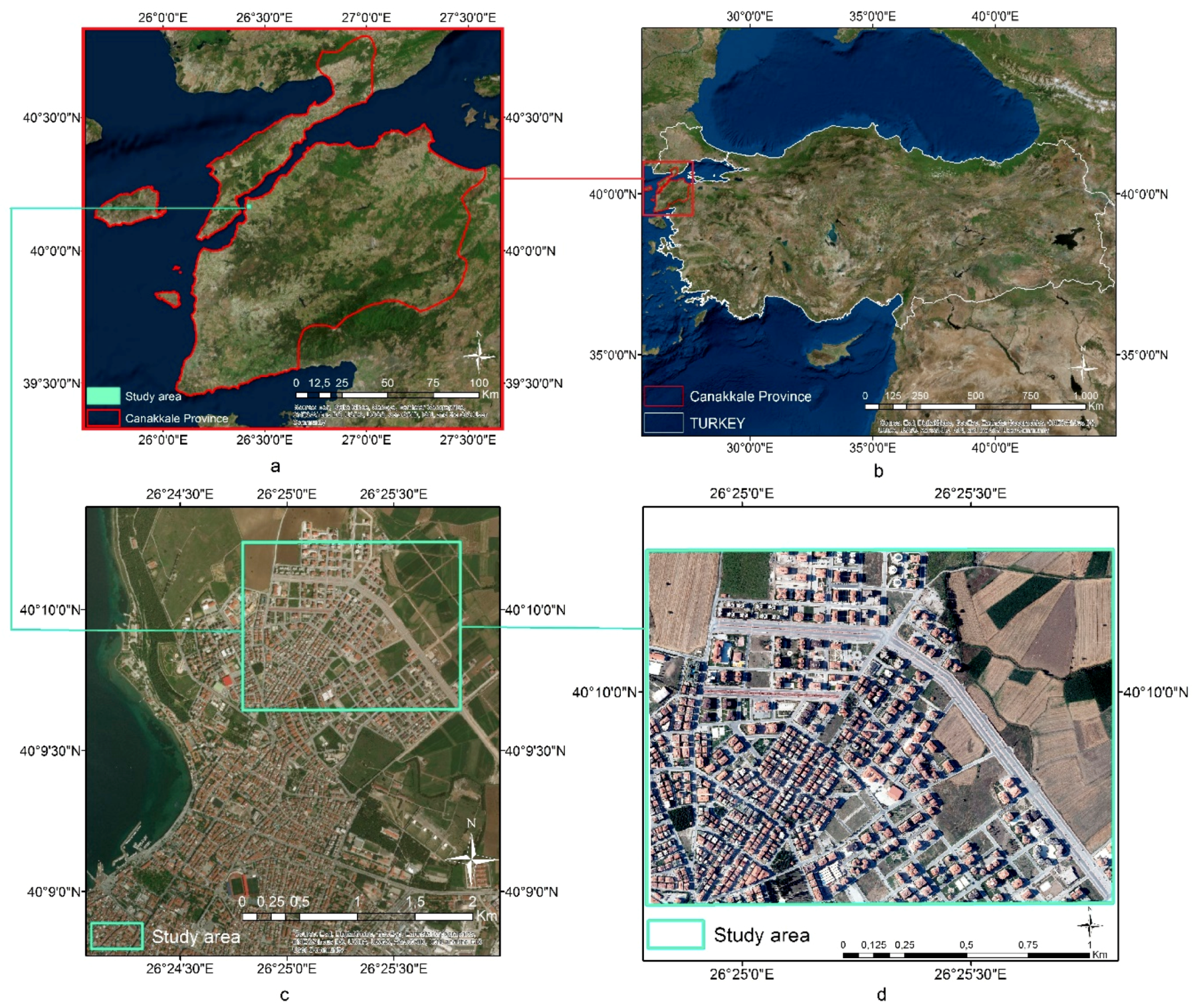
Canakkale province is located between 25°40’–27°30’ E and 39°27’–40°45’ N on both sides of the Dardanelles Straits in the North-Aegean part of Turkey, combining Asia and Europe. The city of Canakkale has dramatically expanded through north and south due to urban development in recent years. The study area (≈160 ha) was selected on the northern edge of the city depending on the variations in LULC types. A relatively low residential density in the newly-developed area, enabling discrimination of buildings, roads, green areas, concrete, and bare soils, was the main criteria for selection of the study area (Figure 1).
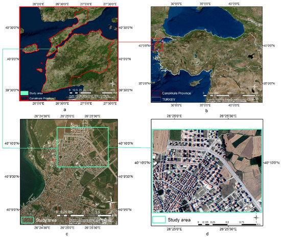
Figure 1.
Study area: (a–c) Google Earth imagery, (d) ortho-mosaic image.
Aerial images at 30 cm ground sample distance acquired by Microsoft UltraCam Eagle photogrammetric digital aerial camera (Table 1) over the city of Çanakkale, Turkey were used to produce orthophotos. For this purpose, each aerial image 30% vertically and 60% horizontally overlaps neighboring images. Initial exterior orientation parameters were estimated by onboard global positioning systems (GPS) and an inertial measurement unit (IMU) system during image acquisition. Initial exterior orientation parameters were adjusted to calculate accurately the exterior orientation parameters of each image using ground control points. In order to produce ortho-images with four spectral bands (red, green, blue (RGB), and near infrared (NIR)), oriented images were used. The mosaic image was generated from these orthophotos with horizontal accuracy of mosaic images within ±2 m based on a 90% confidence interval (Table 2). Then, the study area was clipped from the mosaic image.

Table 1.
Microsoft UltraCam Eagle photogrammetric large-format digital aerial camera specification.

Table 2.
Mosaic image features obtained using photogrammetric process.
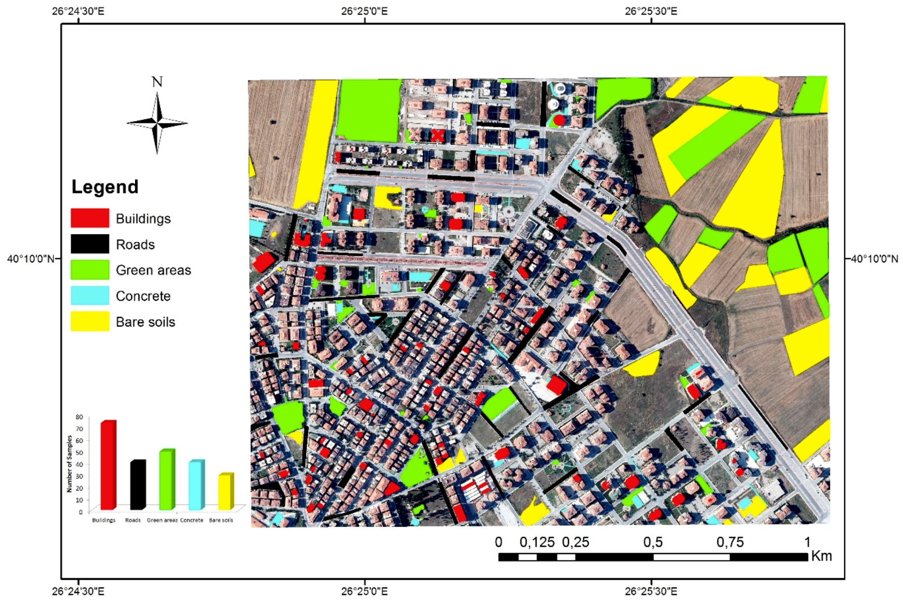
As cited in Reference [40], selection of the training set, and sufficiency of its size and completeness are challenging points in OBIA classification as well as pixel-based approaches [41,42,43,44]. Samples were collected manually depending on the magnitude and homogeneity of patches for each class. In this context, it could be seen that patches are larger and spectrally more homogenous for the bare soil class whereas buildings have varied types of roofing material and shape. Therefore, less samples were able to represent discrimination of the bare class from the others, while buildings required more samples. On the other hand, distribution of the patch size and spectral properties of the green spaces (agriculture and recreation areas), roads (asphalt, with/without shadow), and concrete areas (sidewalks and interlocking pavers) were homogenous compared to the building class. This leads to the approximate number of samples for the mentioned classes in Figure 2.

Figure 2.
Sample distribution of LULC classes.
In OBIA classification, segments as image objects are interpreted based on their object features and thus segments that overlap delineated samples are considered as training and validation samples in OBIA. For the sake of clarity, segments that represent defined samples will be called sample-segments in the remainder of this paper.
3. Methodology
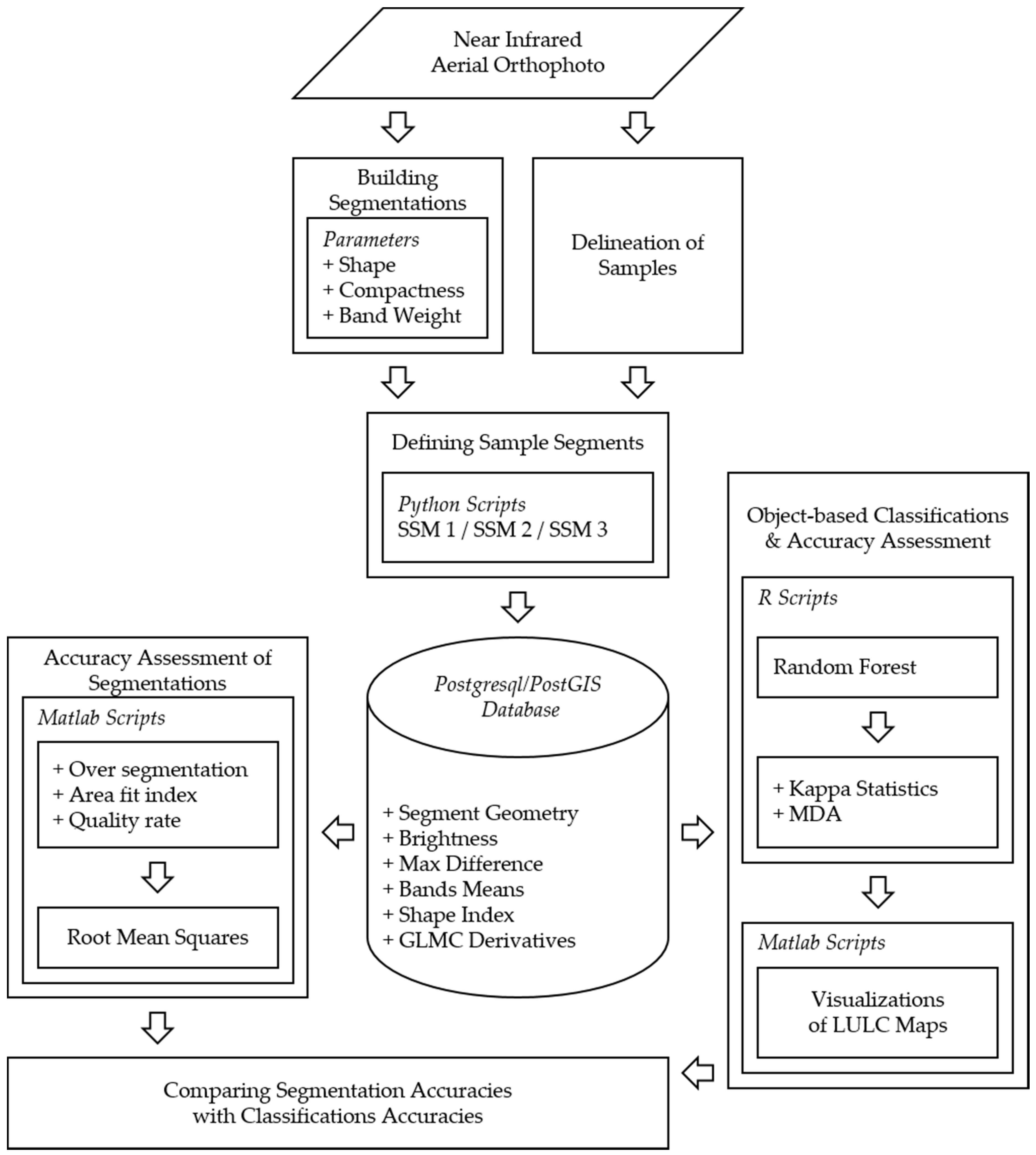
Separately designed subsections constituted the complete methodology of this study (Figure 3). The four band orthophoto explained in the previous section was used as the input. The segmentations and classification samples were determined in the first step. Then, three sample segmentation methods (SSM) were applied using Python scripts to define samples for object-oriented classification. Afterward, recently generated data including object features and the geometries of segments were transferred to the PostgreSQL 9.6.0/PostGIS 2.5 database. The geospatial datasets organized in the PostGIS database were handled in two separate analyses. The first analysis, implemented in Matlab R2016a, concerned segments and segmentation accuracy; whereas the second analysis, produced in R 3.5.1 software, was for random forest classification [45]. Subsequently, LULC maps based on the assignment of image objects to classes were illustrated in Matlab. Finally, segmentation and classification accuracies were examined numerically and compared graphically.
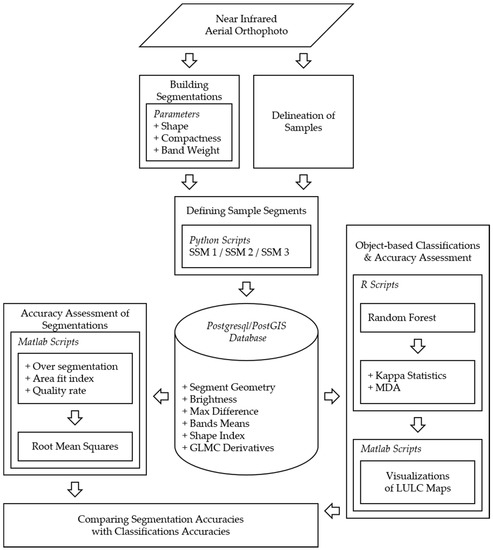
Figure 3.
Workflow diagram.
In general, the outcome of the multi-resolution segmentation algorithm is managed by three main factors: scale, shape, and compactness. For the purpose of this study, weighted bands were also considered in addition to shape and compactness. Both shape and compactness were assessed as 0.1, 0.3, 0.5, 0.7, and 0.9 while the scale value was constant. The optimized scale level 65 was determined using the estimation of scale parameter (ESP) tool, which was introduced in Reference [46] and enhanced in Reference [18]. ESP is an iterative tool that calculates the local variance of image-objects for each scale step starting from the user-defined starting scale parameter. Due to insignificant changes and a large amount of data, 0.3 and 0.7 were eliminated. In order to analyze spectral effects in the segmentation process, single band or multiple bands were weighted. When all these combinations are considered, a total of 108 segmentation attempts was implemented. These segmentation attempts were enumerated from 1 to 108 as their segmentation number (SN). Table 3 presents the shape and compactness criteria and weighted bands for each attempt whereas S, C, and WB indicate shape, compactness, and weighted bands, respectively.

Table 3.
Produced segmentations using different parameters.
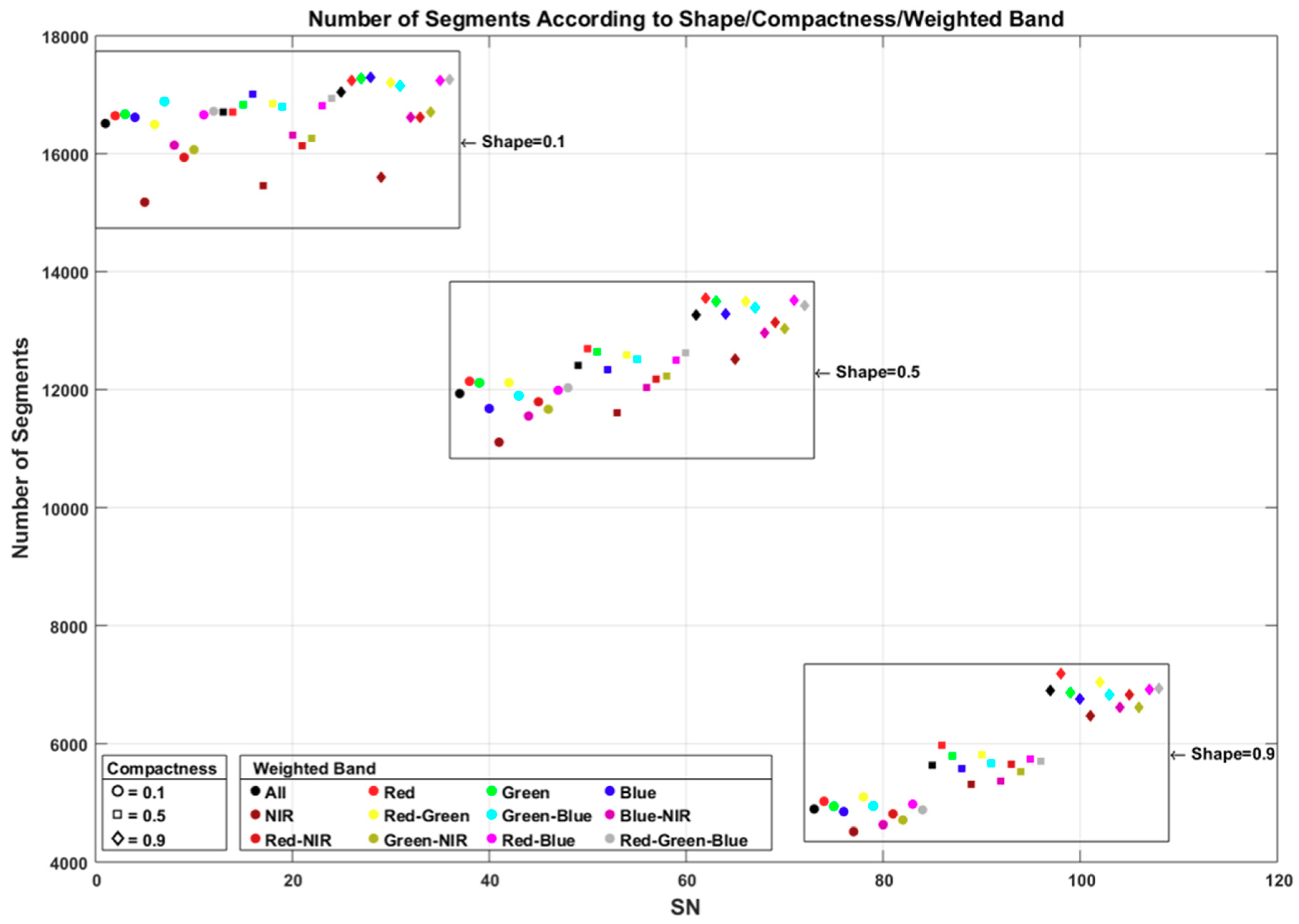
The number of segments for each SN is given in Figure 4. Since shape is known to be the most influential criterion, the number of segments decreased while the shape criteria increased. When the shape was stabilized, increase in compactness led to a higher number of segments. In addition to the above, a decrease in the number of segments was observed by weighting the NIR band. In contrast, the weighted red band increased the number of segments.
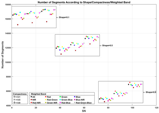
Figure 4.
Number of segments according to segmentation parameters.
In Figure 5, the effects of shape and compactness and the weighting bands on segmentation are demonstrated. Figure 5b presents SN 1 with a shape of 0.1, compactness of 0.1, and each band has the same weight. The segmentation attempt produced 16514 segments with these criteria. With the same compactness and band weights, SN 73 (Figure 5c) produced only 4892 segments with the shape criterion of 0.9. When Figure 5c,d is compared, the enhancing effect of compactness on the number of segments can be seen. With the same shape and band weights for SN 73 (Figure 5c) and SN 97 (Figure 5d), SN 97 had 6904 segments while the compactness was 0.9. SN 98 (Figure 5e) and SN 101 (Figure 5f) indicate the band weighting effects for red and NIR. The number of segments is 7178 and 6463, respectively.
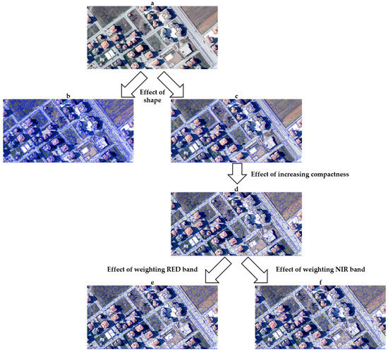
Figure 5.
Comparison of segmentation attempts: (a) southeast of the study area, (b) SN 1, (c) SN 73, (d) SN 97, (e) SN 98, and (f) SN 101.
Although there is no standard approach for image segmentation accuracy assessment, Reference [47] summarized image segmentation accuracy in two main categories, namely, the empirical discrepancy (supervised) and empirical goodness (unsupervised) methods. Then, Reference [22] tabularized the most common related studies with their metrics and references. In this study, over segmentation, area fit index, and quality rate assessment were considered, then the root mean square error (RMSE) was calculated using these assessment values (Equation (4)). Noting that indicates the sample of the total samples and indicates segment of the total intersecting segments with the sample, these assessments are explained as follows:
- Oversegmentation assessment was proposed by Reference [23] and applied in References [48,49]. Oversegmentation of a single sample can be defined as subtracting the division of the total intersecting area of the sample and segments from one (Equation (5)). The overall oversegmentation of the segmentation can be calculated using the means of all (Equation (6)). and have a range between 0 and 1, with 0 as a perfect match.
- Area fit index assessment was proposed by Reference [50] and applied in References [23,51,52]. The area fit index of a single sample can be defined as dividing the sum of the subtracted segments from the sample area by the sample area (Equation (7)). The overall oversegmentation of the segmentation can be calculated by the means of all (Equation (8)). and have a range between 0 and 1, with 0 as a perfect match.
- Quality rate assessment was proposed by Reference [53] and applied in References [48,54,55]. The quality rate of a single sample can be defined as dividing the total intersecting area of the sample and the segments by the union area of the sample and the segments (Equation (9)). The overall over segmentation of the segmentation can be calculated by the means of all (Equation (10)). and have a range between 0 and 1, with 1 as a perfect match.
In this study, the machine learning algorithm called random forest, which yields relatively more accurate results than other classifiers [56], was preferred to label undefined urban image objects of distinctive segmentation. Another reason for choosing random forest is its ability to handle a large data set with higher dimensionality. Random forest as an ensemble classifier works with a large collection of de-correlated decision trees. One third of the samples, also known as out-of-bag (OOB) samples, are used in an internal cross-validation technique for OOB error estimation. While M and N denote, respectively, the total number of input variables and the number of trees, six essential steps to implement the random forest classification algorithm can be explained briefly as follows [57]:
- Randomly select m variable subsets from M where m < M.
- Calculate the best split point among the m feature for node d.
- Divide the node into two nodes using the best split.
- Repeat the first three steps until a certain number of nodes has been reached.
- Repeat the first four steps to build the forest N times.
- Predict new observations with a majority vote.
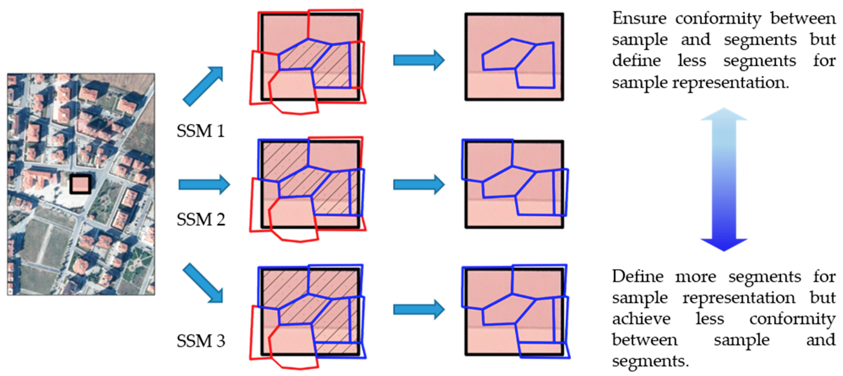
Labeled segments, which represent delineated samples as training data, were defined in three categories by the distinct segment selection method (Table 4). Segment selection methods (SSM) differ depending on the ratio calculated using the overlap area between segments and delineated samples. If a training segment is totally covered by a sample, in other words no points of a segment geometrically lie in the exterior of a sample, it is called SSM 1. If a segment maximally overflows a sample by 10% of the overlap area, it is called SSM 2. In addition, if a segment maximally overflows a sample by 20% of the overlap area, it is called SSM 3. Figure 6 shows labeled training segments from a building sample using the three distinct criteria.

Table 4.
Three criteria for training segment definition.
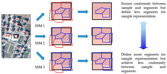
Figure 6.
Defining training segments using different criteria.
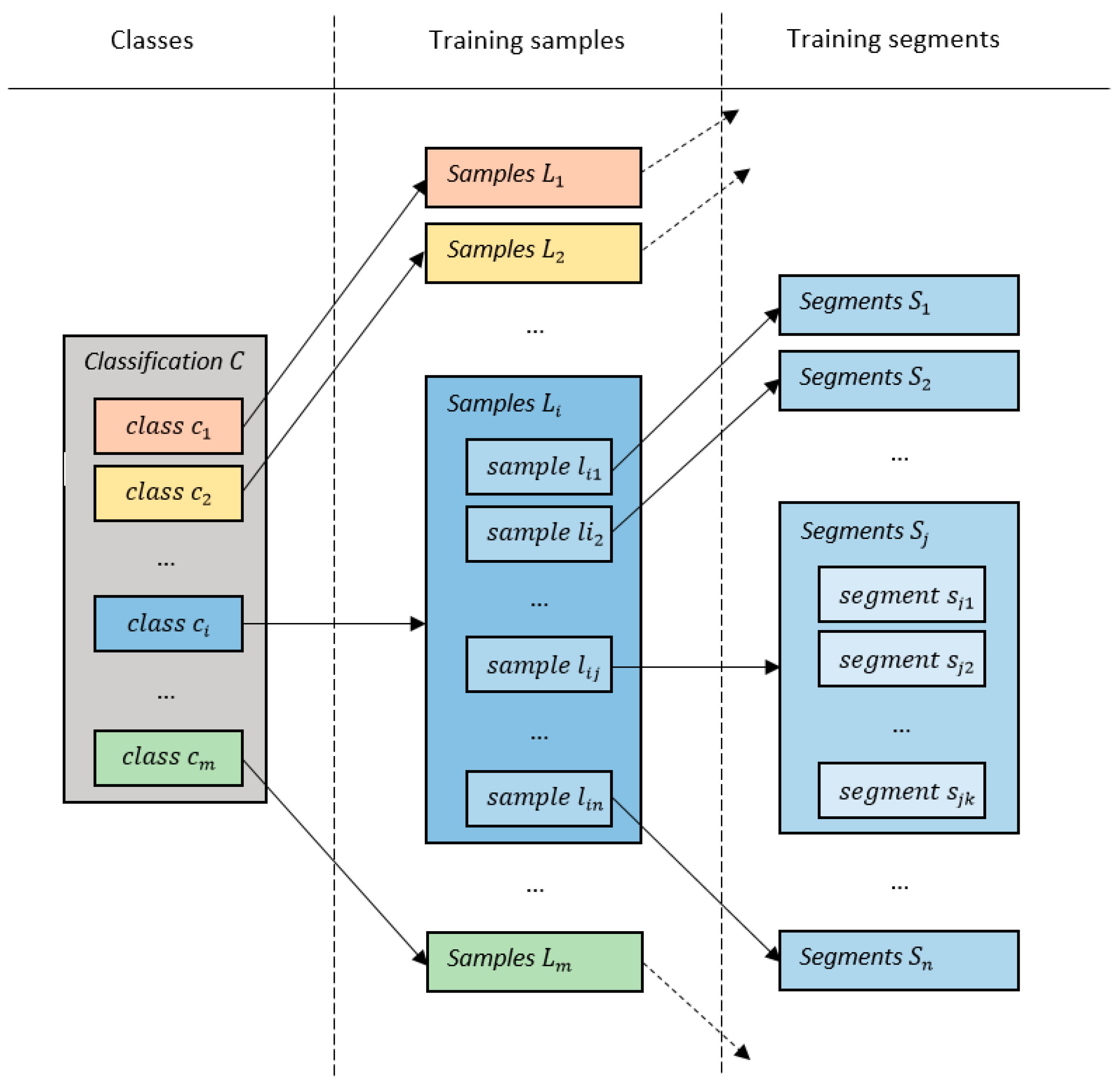
LULC classification can be expressed as and indicates any class of whereas indicates the total number of classes in . Training samples , defined as representative of any class , can be written as , where indicates the sample of class . Moreover, labeled training segments are explained as where indicates the total number of overlapping segments satisfying the criterion with sample (Figure 7). When the three different SSMs are considered, the implementation of 324 random forest classifications, three times the 108 segmentations, were predicted in this study.
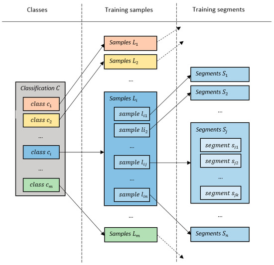
Figure 7.
Class, sample and segment relations.
Many and various object features, which are based on spectral information, shape, texture, geometry, and contextual semantic knowledge, can be selected to classify image objects after the segmentation step is implemented in OBIA. In total, fourteen variables—mean values of band layers, maximum difference, brightness, GLCM (gray-level co-occurrence matrix) derivatives, and shape index—as significant object features in LULC classifications [21,58,59] were used in this study (Table 5). Each GCLM measure was calculated using the mean value of red, green, blue, and NIR band values.

Table 5.
Image object features used as classification variables.
4. Results and Discussion
4.1. Segmentation Accuracy
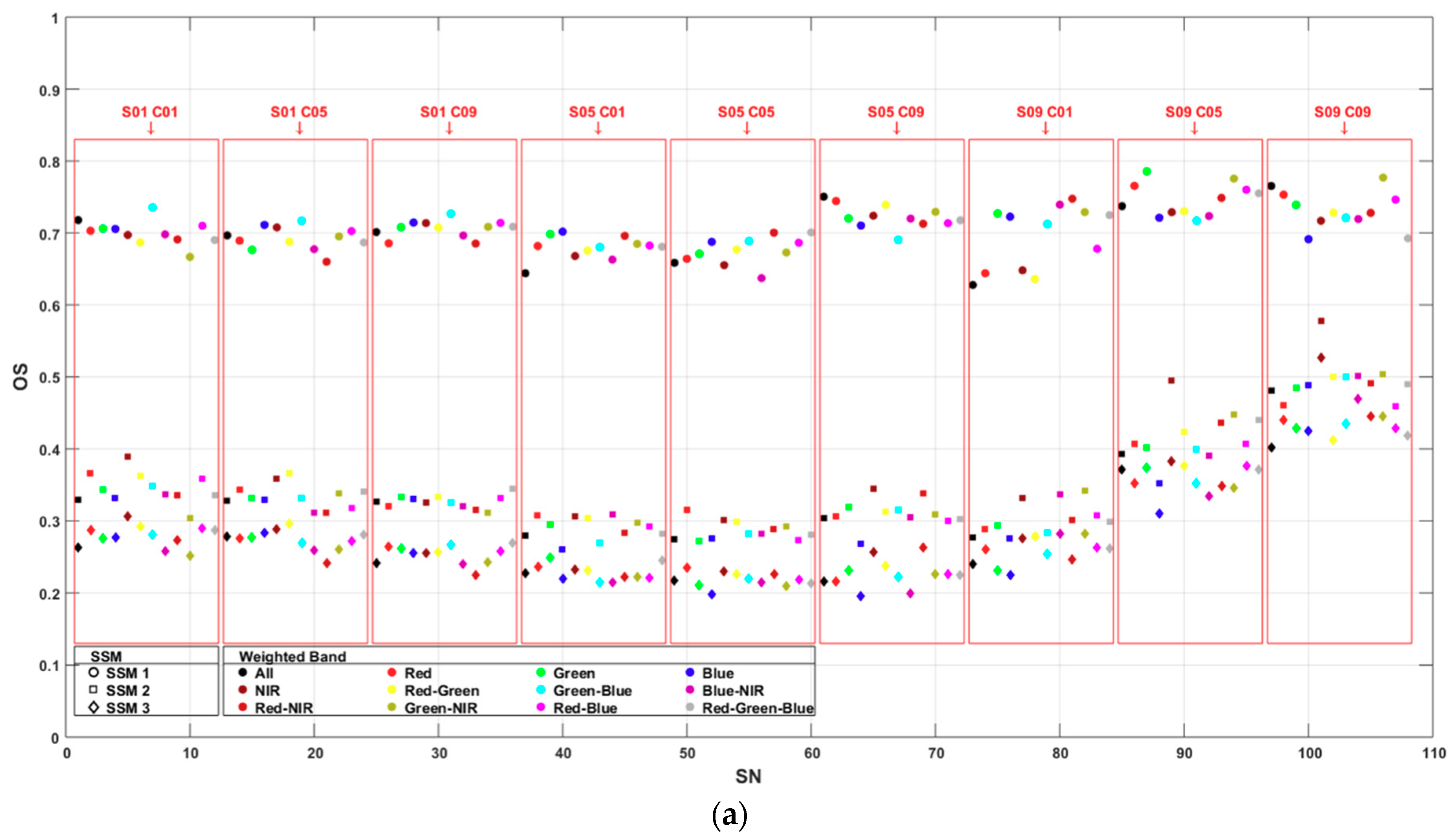
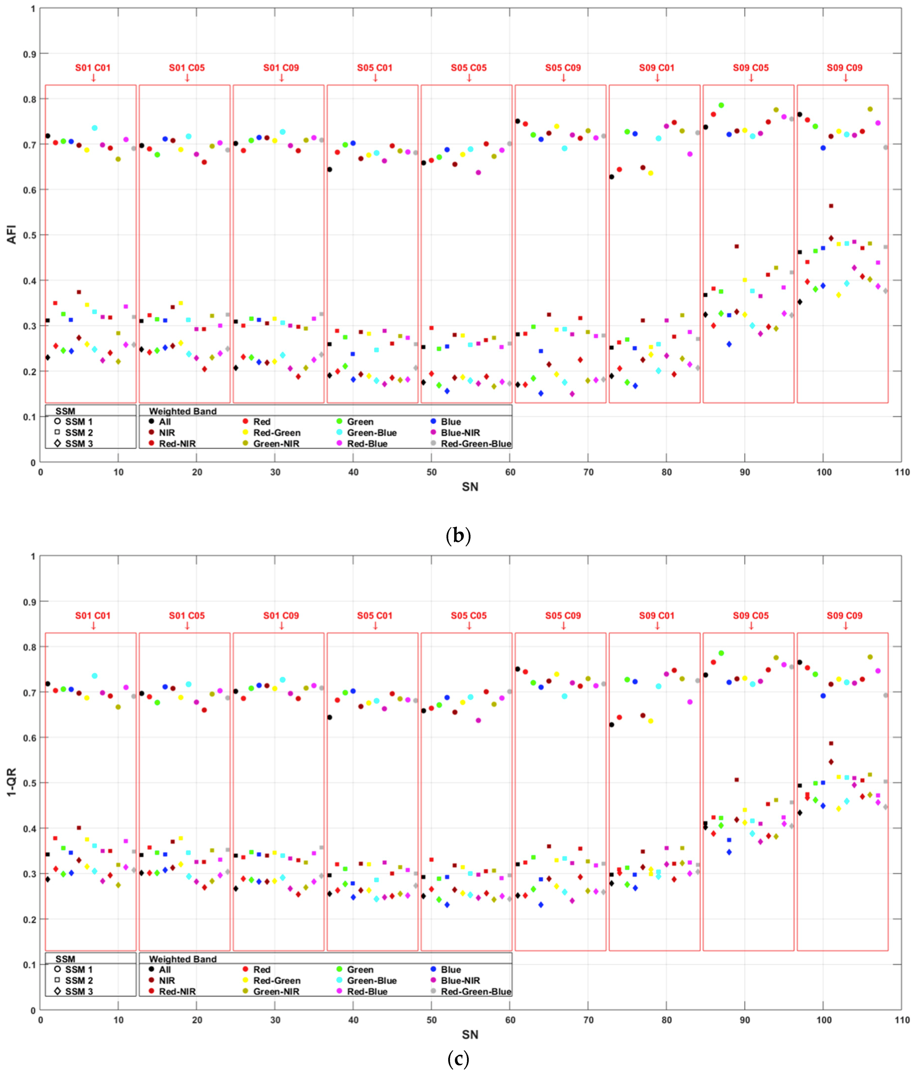
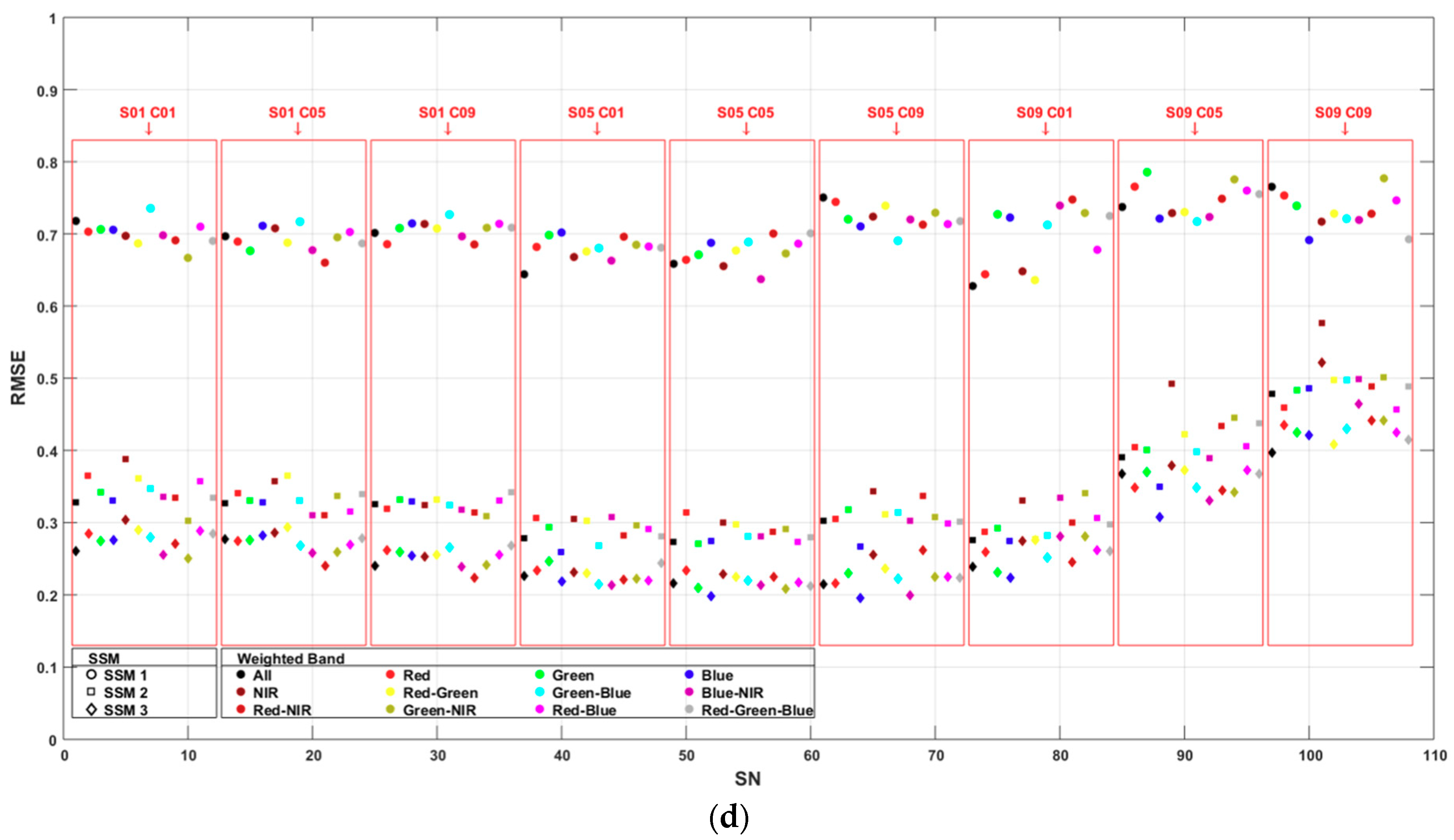
As the first step of segmentation accuracy analysis, OS, AFI, and QR assessment criteria were evaluated (Figure 8a–c). It can be clearly seen that their distribution showed almost the same trends. To reduce the random error, the RMSE criterion proposed in this study was used as a combination of these three assessments. Figure 8a–d illustrate that RMSE resulted in low accuracies for SSM 1 when compared to SSM 2 and SSM 3. As indicated before, this emerged from the inadequate representation of samples by SSM 1. Also, the shape and compactness criteria and the weighted band effect on segment accuracy could not be sufficiently distinguished in SSM 1.
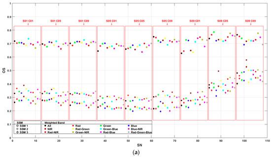
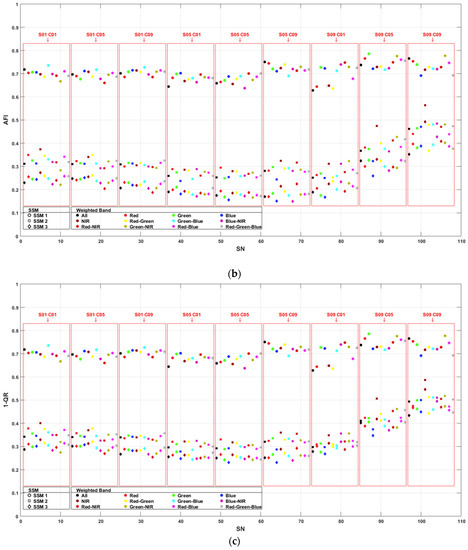
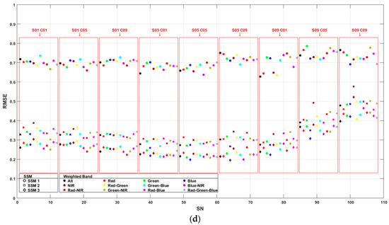
Figure 8.
(a) Over segmentation, (b) area fit index, (c) 1-Quality rate, and (d) root mean square error of segmentations.
When SSM 2 and SSM 3 were compared, it could be stated that SSM 3 produced higher accuracies with an average of 6% OS, 8% AFI, 5% QR, and 6% RMSE. On the other hand, when the value changes in shape and compactness and the weighted band were considered, similar behaviors in accuracy were observed in SSM 2 and SSM 3. For both methods, lower RMSE values were obtained with 0.5 shape values. Higher shape values needed higher compactness values in order to produce low RMSE values when the compactness changes were individually examined. Although band weighting affected RMSE only slightly; the weighted NIR band caused a moderate reduction in accuracy. Particularly, the equally weighted and the red-NIR-weighted bands achieved high accuracy in segmentation parameters S01, producing small segment sizes, whereas blue-weighted band segmentation in S05 and S09 was noticed to be the most accurate.
4.2. Classification Accuracy
As shown in Table 6, 257 out of 324 classifications were successfully implemented in the study. Due to the considerable increase in segment size at high shape values, SSM 1 provided low sample-segment numbers that strongly influence the classifications. Moreover, it is observed that SSM 2 also caused failure on 17 classifications. Sample-segments obtained by SSM 3 successfully accomplished the remained 108 classifications.

Table 6.
Number of random forest classifications.
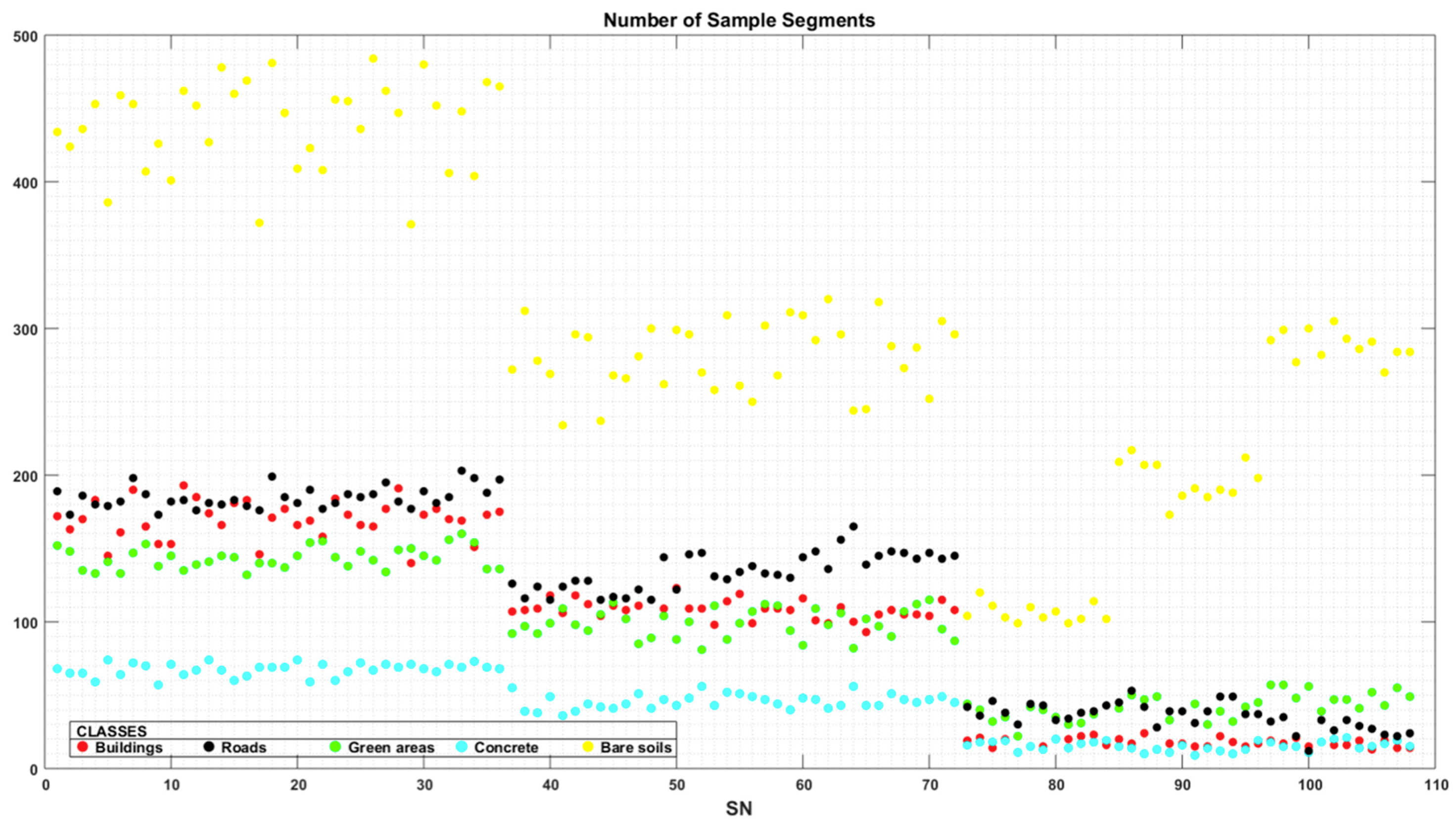
When considering the number of sample-segments in the OBIA classification, sample-segments for each class were determined properly according to the size of the collected samples and segmentation parameters (Figure 9). Additionally, the number of sample-segments was proportional to the total number of segments of each segmentation attempt. It was also noted that the ratio between the number of sample-segments and total number of segments of each segmentation remained nearly unchanged. Thus, the ratio which trivialized the differences in the number of sample-segments also protected the number of assignments to the training number for each classification.
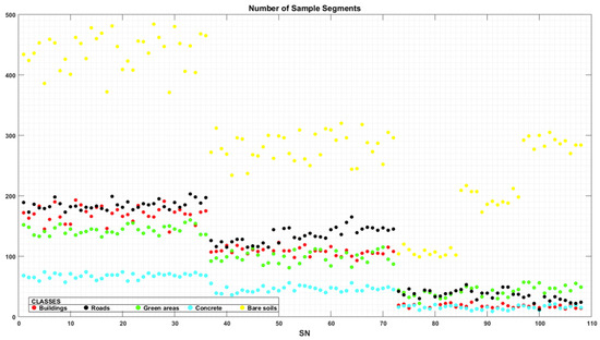
Figure 9.
Number of sample-segments for each class in classifications based on SSM 3.
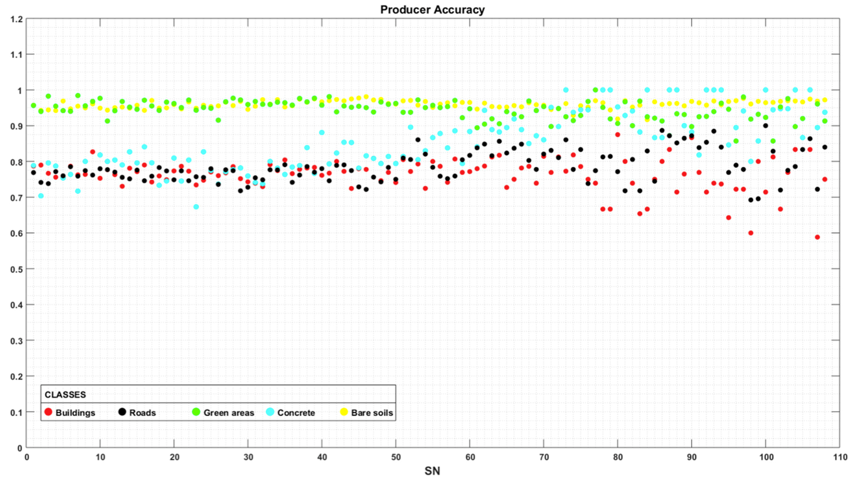
The error matrix, also known as the confusion matrix, is one of the most-used accuracy assessment techniques in supervised LULC classification [60]. Both user accuracy and producer accuracy calculated in the error matrix indicate a degree of consistency between class prediction and validation data. Having the largest sample-segment size, user accuracies of error matrices of SSM3 classifications shown in Figure 10 indicate that the bare soil class has almost the highest accuracy in each user accuracy of error matrices. However, bare soil accuracies decreased in S09-C01 while user accuracies for the concrete class obtained higher values. This result indicates that compactness and band weights become more sensitive in high shape values. Moreover, heterogeneous land-use objects, such as buildings and roads, were significantly affected by band weighting, particularly at high shape values. The determined effect was also observed partly in producer accuracies of error matrices (Figure 11).
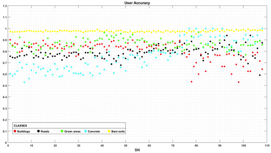
Figure 10.
User accuracies for each class in classifications based on SSM 3.

Figure 11.
Producer accuracies for each class in classifications based on SSM 3.
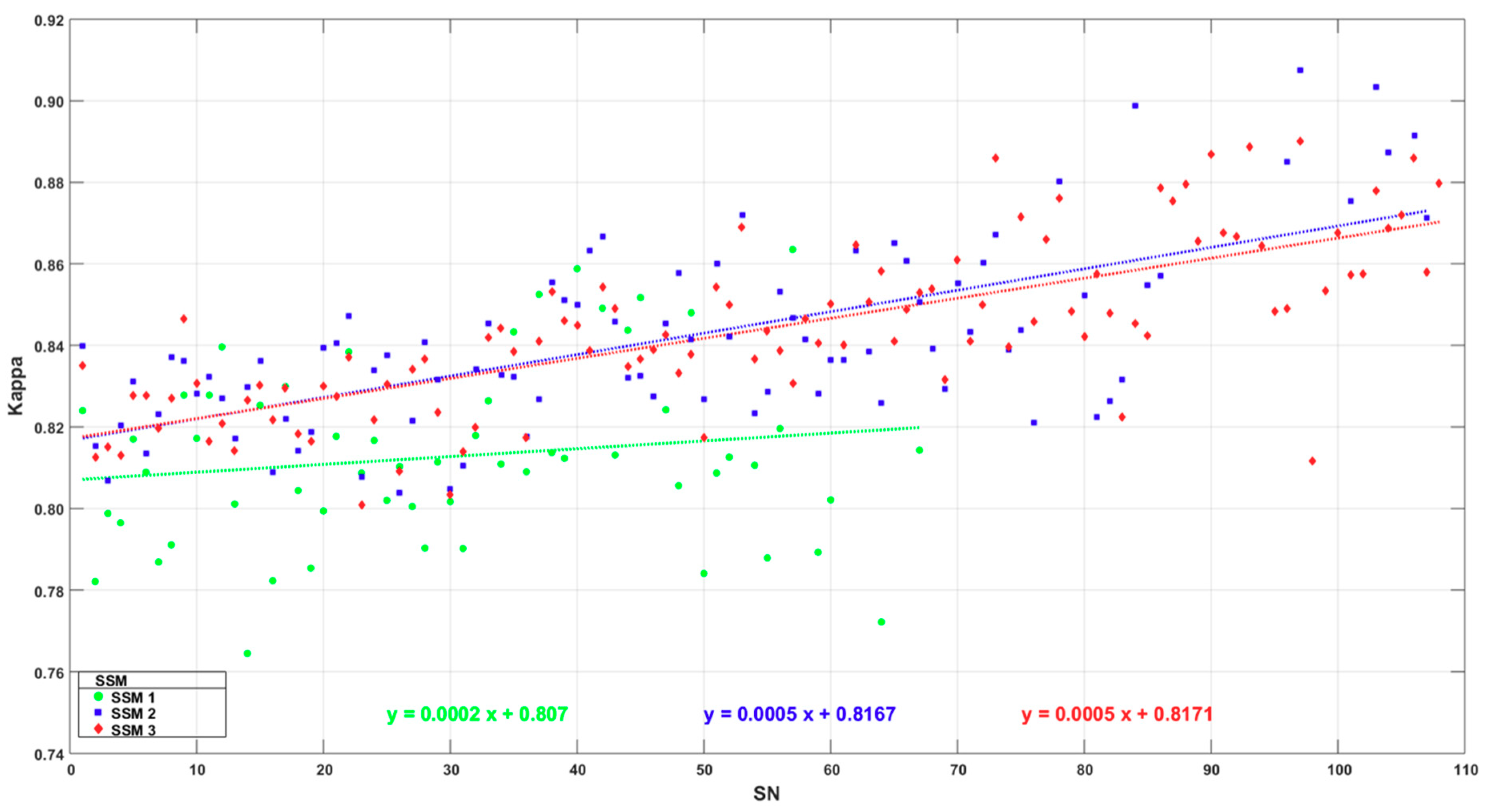
The kappa index produced from the error matrix determined the correspondence between prediction values and actual values as an accuracy criterion. Obtained kappa values (color-based on SSMs) are seen in Figure 12 as a result of random forest classifications. According to the figure, it is seen that the higher the shape value of the segmentation, the greater the kappa accuracy of the classification produced. The slope coefficient of the equation by SSM 1 was lower than those of SSM 2 and SSM 3 when the linear regressions were examined in Figure 12. Most likely, the missing classifications belonging to the higher shape values in SSM 1 caused a decrease in the slope coefficient of the equation SSM 1. On the other hand, when the intercept values were considered, SSM 2 and SSM 3 presented higher kappa values than SSM 1. In addition, the slope coefficient of the equations by SSM 2 and SSM 3 were quite close to each other. The kappa results briefly indicated that SSM 2 and SSM 3 had a similar effect on classification accuracy and led to greater accuracy than SSM 1.
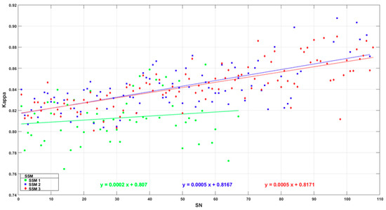
Figure 12.
Kappa values according to segmentation numbers.
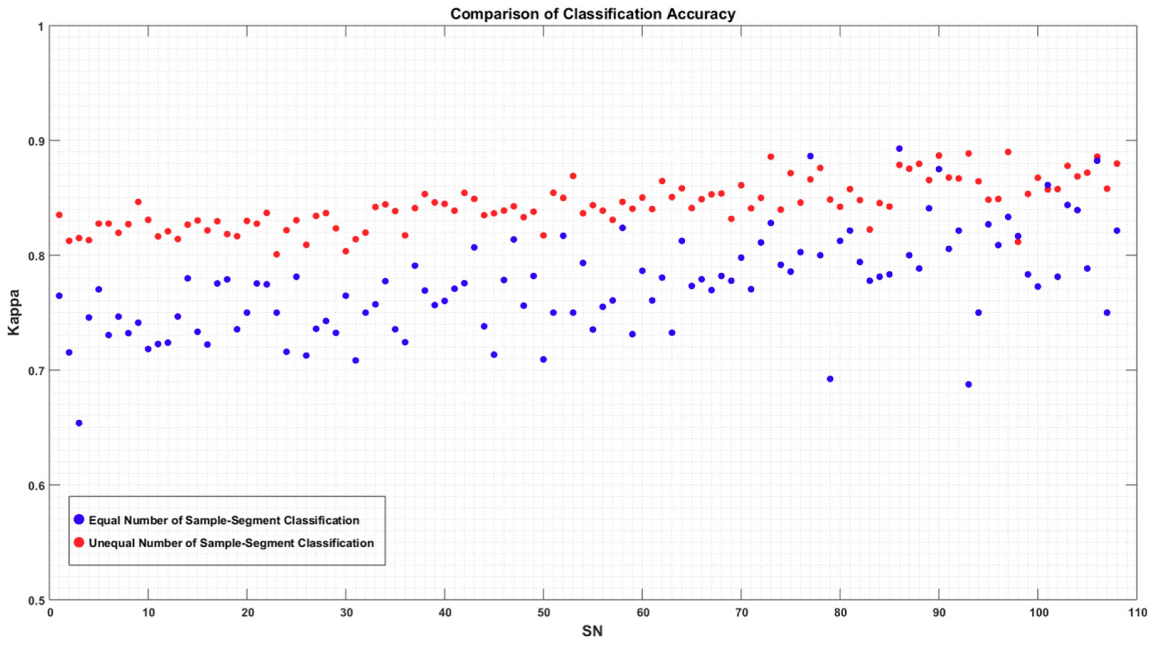
In the study, inconsistency among the number of sample-segments for each class was also considered. For example, buildings, green areas, roads, concrete, and bare soils as depicted in Figure 9 have a different number of sample-segments for the implemented classifications; this is called unequally-sampled classifications. An equal number of subset sample-segments for each class was randomly selected and then classifications were also implemented. The kappa indices computed from equally-sampled classifications were compared with the previous unequally-sampled classifications produced using SSM 3. Although equally-sampled classifications achieved lower accuracies than unequally-sampled classifications (Figure 13), the two types of classification, having different sampling, showed a generally similar tendency in kappa accuracies due to the increasing shape parameter value. It was also seen that accuracies became closer at higher shape values except for some band weighting. Moreover, major accuracy changes occurred among equally-sampled classification due to segmentation parameters.
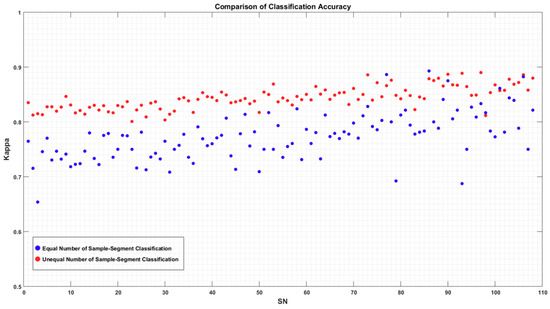
Figure 13.
Comparison of classification accuracies of equal and unequal number of sample-segment classifications based on SSM 3.
4.3. Variable Importance
In the random forest classification, mean decrease accuracy (MDA) and Gini index are the two most-used algorithms for calculating variable importance measures [57,61,62]. In this study, MDA, which evaluates and sorts the variable effect on classification accuracy, was used to interpret the relation between segmentation criterion and classification variables. For each classification, the most important three out of fourteen variables (Table 5) were determined. Furthermore, 254 classifications were categorized based on their segmentation criteria, and percentages of the variable appearance were computed (Figure 14).
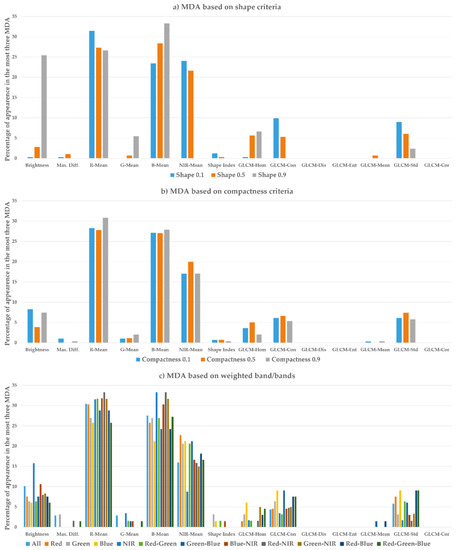
Figure 14.
Mean decrease accuracy for variables.
As shown in Figure 14a–c, RMean and BMean were the most effective variables in these classifications. It was also observed that Brightness, NIRMean, GLCMHom, GLCMCon, and GLCMStd variables had a moderate impact. Particularly, increasing the shape value led to boosting the Brightness and GLCMHom variables; however, the importance of NIRMean, GLCMCon, and GLCMStd variables dramatically dropped in Figure 14a. As compactness and band weighting did not influence segmentation as much as shape, these criteria did not have a continuous effect in variable importance (Figure 14b,c). Furthermore, a significant impact of the brightness variable in OBIA LULC classification based on NIR-weighted segmentation was determined.
The bias possibility in MDA was also considered due to correlated predictor variables such as textural measures. Thus, a conditional permutation importance measure able to evaluate the importance of correlated predictor variables was calculated using R Package Party [63,64]. The results showed that random forest implementation utilizing conditional inference trees generally produced consistent results with R package RandomForest based on References [45,57]. Furthermore, minor changes occurred in the determination of the three most important variables using conditional variable importance. It is also recommended that conditional variable importance should be taken into account in more detailed discussion of uncorrelated variable importance.
4.4. Classification Results
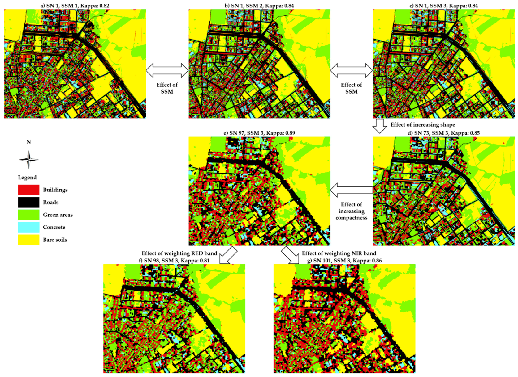
Figure 15 presents classification maps for various SSM and segmentation criteria. Especially, buildings with shadows on the ground could not be detected separately as different classes using SSM 1 (Figure 15a) due to inadequate sample representation by segments. Maps produced from SSM 2 (Figure 15b) and SSM 3 (Figure 15c) were quite similar, whereas the first row of Figure 15 shows differences in classification among SSMs. The effect of the shape value increase on the classification maps is seen between Figure 15c and Figure 15d. Objects with larger areas were appropriately classified, while there were random errors for small area objects because of the high resolution. On the other hand, increasing compactness causes a salt and pepper effect, as depicted in Figure 15e. Furthermore, due to changes in the band weighting, some object types become more dominant in classification, such as the NIR favored building class.
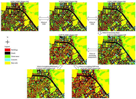
Figure 15.
Classification examples.
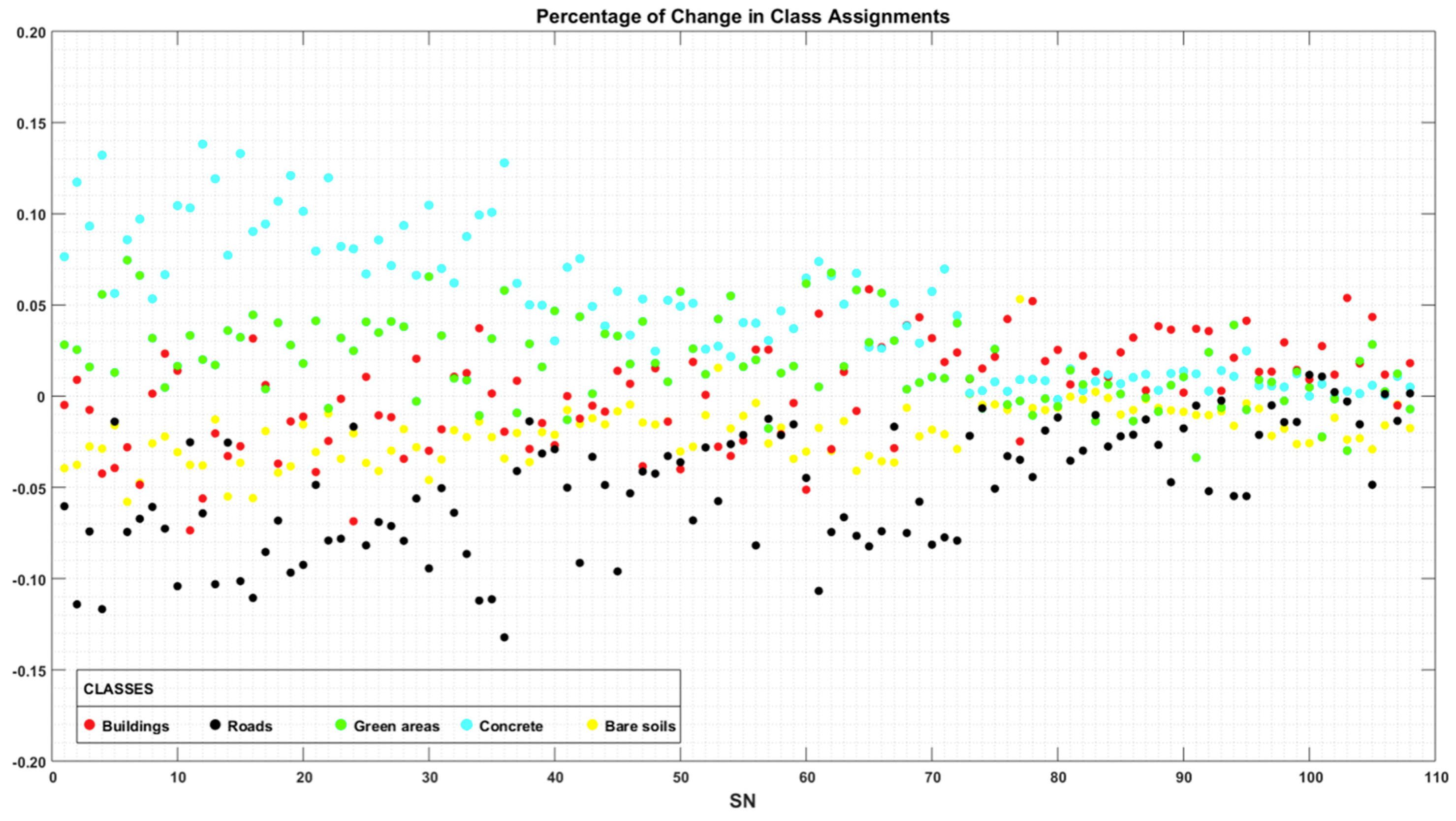
The influence of the absolute sample size on class assignment obtained from classification predictions was examined using Figure 16. Substantial differences in class assignment were achieved between unequally and equally-sampled classifications at low shape values. Positive and negative changes were especially determined between concrete and road classes. Positive change referred to more assignments in classes with equal sampling whereas negative ones indicated an increase in assignments in classes with unequal sampling. In this context, bare soil assignments were not influenced exclusively, although that class had more sample-segments than others. On the other hand, segments were mostly predicted as roads under unequally sampling, despite the class having a moderate number of sample-segments compared to other classes. Moreover, concrete was determined as the most influenced class due to its lower number of sample-segments. The results showed that the number of sample-segments was not the unique reason for OBIA classification and class assignments.
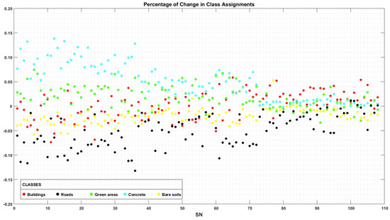
Figure 16.
Percentage of change in class assignment in classifications based on SSM 3.
4.5. Comparison between Segmentation and Classification Accuracies
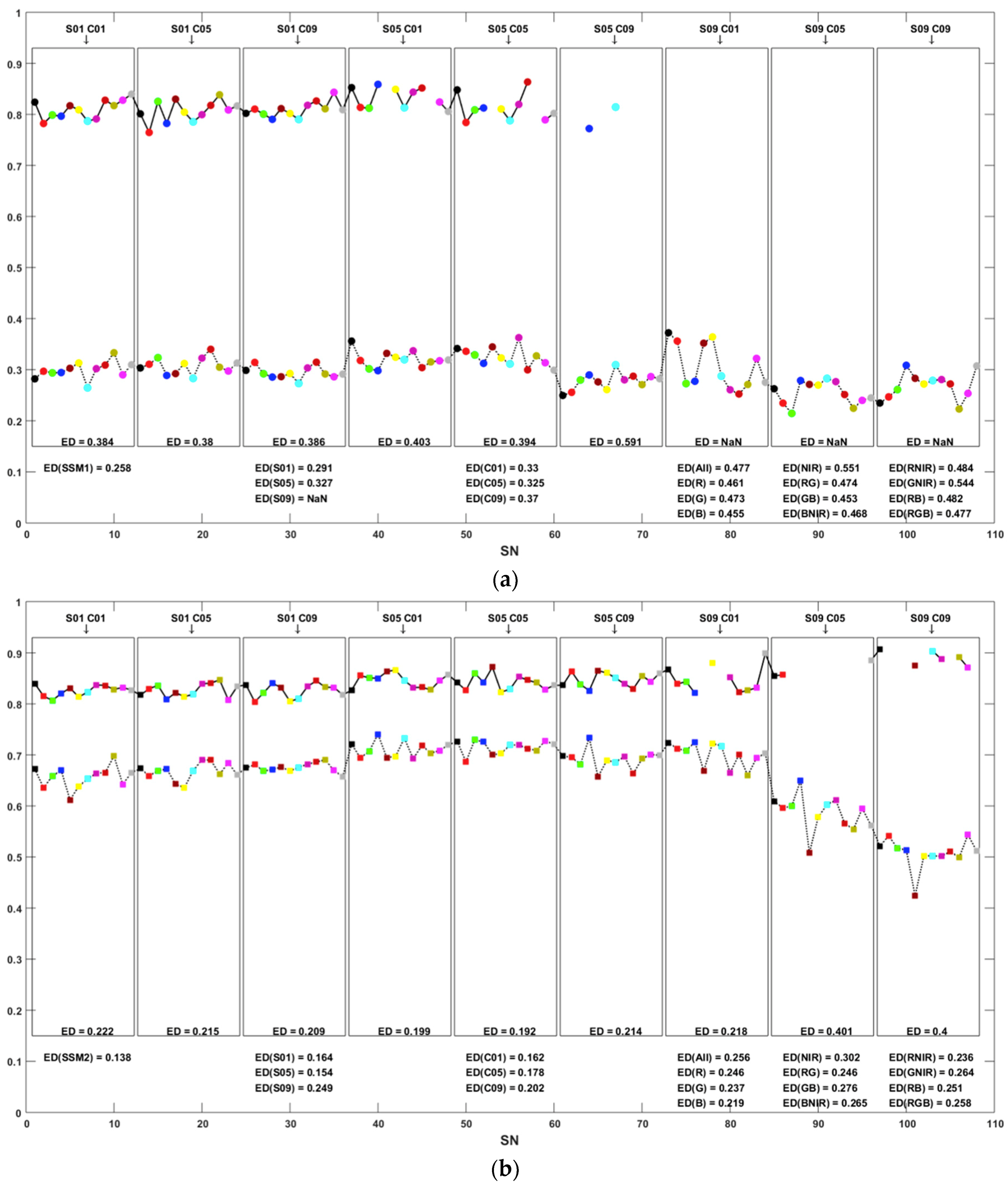
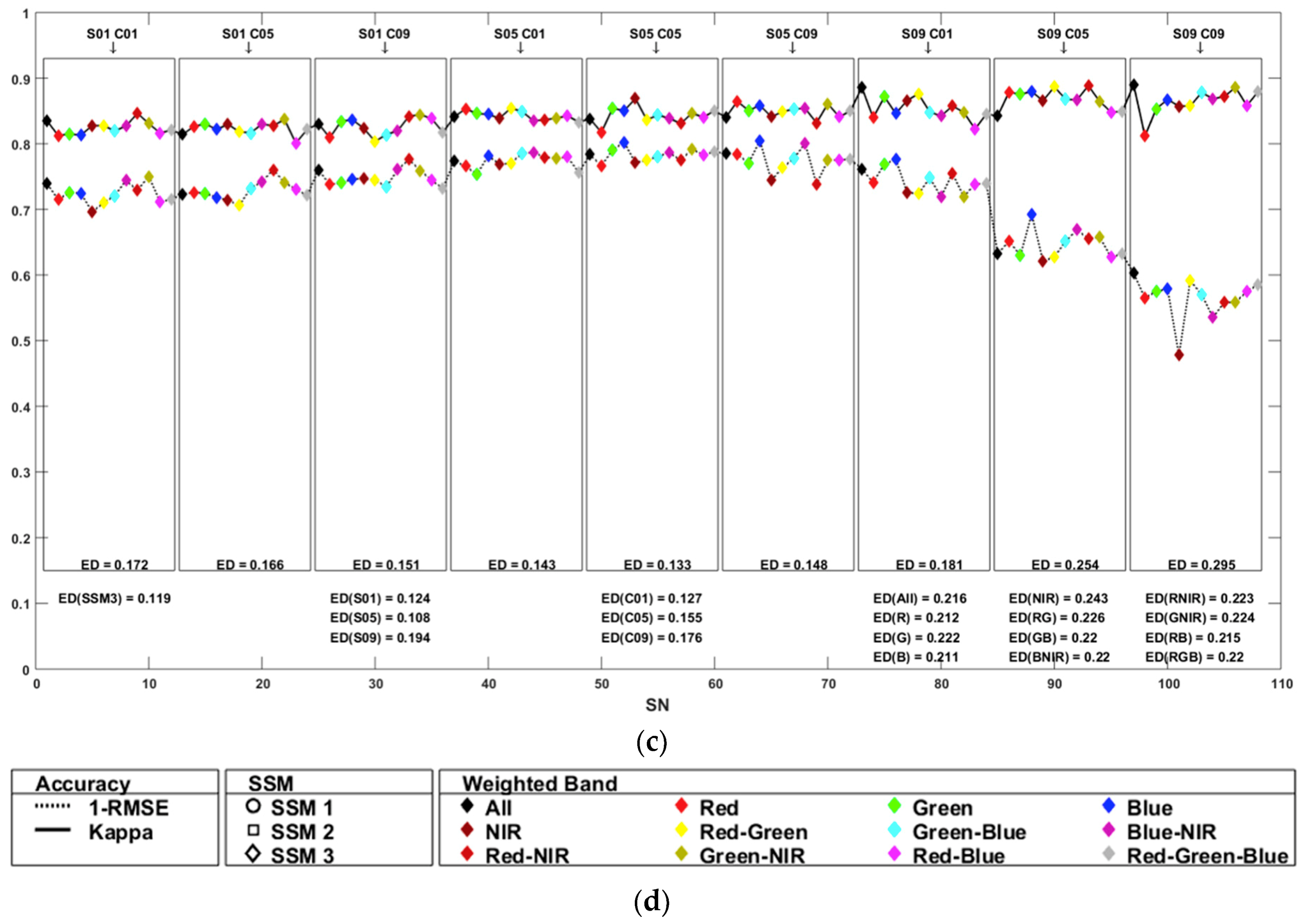
In Figure 17, segmentation RMSE values and classification kappa values were compared to examine the explicit relationship between segmentation accuracy and classification accuracy. Since lower RMSE and higher kappa values indicated better accuracies for segmentation and classification respectively; 1-RMSE is given in Figure 17a–c illustrating SSM 1, 2, and 3, respectively. To provide a comprehensible visualization between RMSE and kappa, each plot was highlighted with boxes defining their shape and compactness values such as S01-C01, S01-C05, and S01-C09. As seen in Figure 17a representing the classifications obtained using SSM 1, S05-C01 and S05-C05 were substantially distinguished by the relative similarities between RMSE and kappa accuracy values. In S01-C05, a partial consistency between RMSE and kappa accuracies was also determined, although it did not as implicitly occur as in S05-C01 and S05-C05. On the other hand, graphical conformity between segmentation and classification accuracy values was seen for S01-C05 and S05-C05 (Figure 17b). Figure 17c mostly illustrates coherence between RSME and kappa values except for all combinations of S09 besides some detected resemblances in both Figure 17a,b. In particular, more conformity between RMSE and kappa values stands out for both S05-C01 and S05-C05 in Figure 17c. Furthermore, Euclidean distances (ED) for each SSM, shape and compactness value, and the weighted bands are given at the bottom-right of the related figure. Moreover, EDs for each highlighted shape and compactness group are given in the boxes. The ED were computed by Equation (11) where represents 1-RMSE, represents kappa, and and are the mean of 1-RMSE and kappa, respectively. Given ED values also solidified the conformities mentioned above.
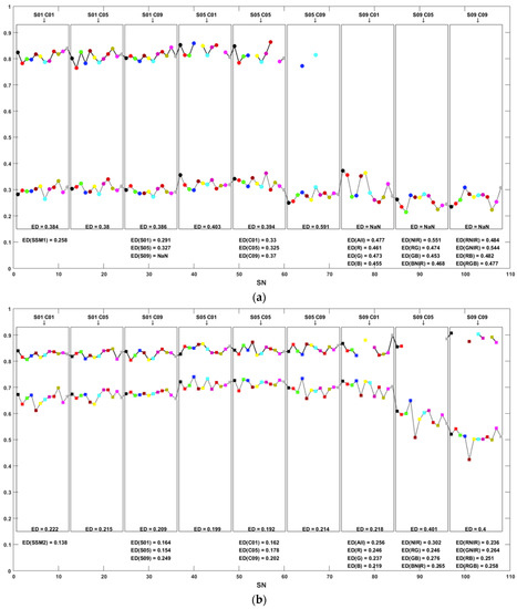
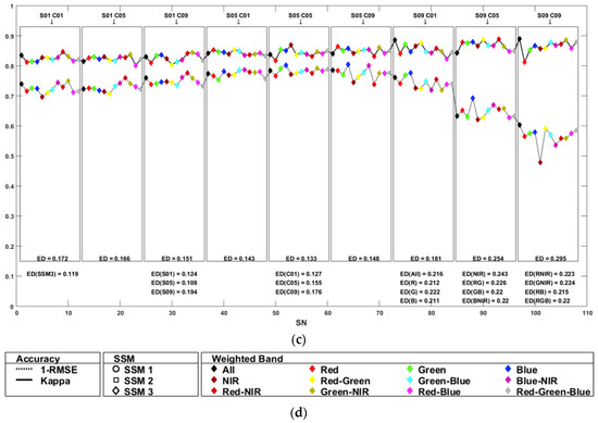
Figure 17.
Classification kappa values and segmentation RMSE values according to segment selection method, shape and compactness criteria and Euclidean distances (a) SSM 1, (b) SSM 2, (c) SSM 3, and (d) legend.
5. Conclusions
In this study, accuracies of multi-resolution segmentation and classification based on different shape, color, compactness, and band-weights were analyzed. The proposed RMSE, defined in this study as a remarkable coexistence of three profoundly different accuracy assessments, delivered more objective and comprehensive segmentation accuracy. Weighting only the NIR band reduced the accuracy of the segmentation. However, due to the high importance of the NIR band in the classification, color-infrared images should be used for newly-developed urban areas.
When sample selection for OBIA is considered, sample-segments overflowing samples by 20% provided more appropriate segment representation for the sample image objects. On the other hand, the ratio of the total number of sample-segments to the total number of segments should not be less than 0.5% for an accurate classification.
In general, a concrete correlation between segmentation and classification accuracies can be stated. However, the largest deviations are expected in classifications derived using high shape values. The compactness value exerted a greater effect when it was used with higher shape values. Kappa indices also prove that high compactness for low shape values and low compactness for high shape values should be selected.
In classification attempts, various segmentation parameters highlighted objects of some classes while partly ignoring the remainder of the objects in other classes. For example, classifications using red band-weighted segmentation led to some object loss in the building class. When all LULC categories are classified using high resolution infrared aerial images, S05-C05 as segmentation parameters and SSM 3 as sample selection method are recommended.
For the future, LULC sub-classes can be considered to highlight the effect of different band combinations on various objects, as the present study was implemented for five classes. Classifications using high resolution satellite images having varied spectral bands and ranges should be discussed and compared to each other to understand the broad relationship between segmentation and object-based classification. Segmentation accuracy assessment methods should also be examined to better reflect object-based classification needs in the future. Impact of different overflow values in sample selection should be considered in terms of image-object representation.
Author Contributions
O.A. and E.O.A. designed the research; A.C. prepared orthophotos; O.A. and E.O.A. performed segmentations; M.I. defined and delineated samples; O.A. designed the geodatabase; E.O.A. computed segmentation accuracies; O.A. analyzed classifications; O.A., E.O.A., M.I., L.G., and A.C. wrote and reviewed the paper.
Funding
This research received no external funding.
Acknowledgments
The authors acknowledge support from the Turkish General Directorate of Mapping in providing high-resolution infrared aerial images within the project “Monitoring of urban-rural development with high-resolution aerial images”.
Conflicts of Interest
The authors declare no conflict of interest.
References
- Saadat, H.; Adamowski, J.; Bonnel, R.; Shafiri, F.; Namdar, M.; Ale-Ebrahim, S. Land use land cover classification over a large area in Iran based on single date analysis of satellite imagery. ISPRS J. Photogramm. 2011, 66, 608–619. [Google Scholar] [CrossRef]
- Tehrany, M.S.; Pradhan, B.; Jebuv, M.N. A comparative assessment between object and pixel-based classification approaches for land use/land cover mapping using SPOT 5 imagery. Geocarto Int. 2013, 29, 351–369. [Google Scholar] [CrossRef]
- Roelfsema, C.M.; Lyons, M.; Kovacs, E.M.; Maxwell, P.; Saunders, M.I.; Samper-Villarreal, J.; Phinn, S.R. Multi-temporal mapping of seagrass cover, species and biomass: A semi-automated object based image analysis approach. Remote Sens. Environ. 2014, 150, 172–187. [Google Scholar] [CrossRef]
- Mafanya, M.; Tsele, P.; Botai, J.; Manyama, P.; Swart, B.; Monate, T. Evaluating pixel and object based image classification techniques for mapping plant invasions from UAV derived aerial imagery: Harrisia pomanensis as a case study. ISPRS J. Photogramm. 2017, 129, 1–11. [Google Scholar] [CrossRef]
- Torres-Sánchez, J.; López-Granados, F.; Peña, J.M. An automatic object-based method for optimal thresholding in UAV images: Application for vegetation detection in herbaceous crops. Comput. Electron. Agric. 2015, 114, 43–52. [Google Scholar] [CrossRef]
- de Alwis Pitts, D.A.; So, E. Enhanced change detection index for disaster response, recovery assessment and monitoring of accessibility and open spaces (camp sites). Int. J. Appl. Earth Obs. 2017, 57, 49–60. [Google Scholar] [CrossRef]
- Blaschke, T. Object based image analysis for remote sensing. ISPRS J. Photogramm. 2010, 65, 2–16. [Google Scholar] [CrossRef]
- Ma, L.; Li, M.; Ma, X.; Cheng, L.; Du, P.; Liu, Y. A review of supervised object-based land-cover image classification. ISPRS J. Photogramm. 2017, 130, 277–293. [Google Scholar] [CrossRef]
- Baatz, M.; Schäpe, A. Multiresolution segmentation: An optimization approach for high quality multi-scale image segmentation. In Angewandte Geographische Informations-Verarbeitung XII; Strobl, J., Blaschke, T., Griesbner, G., Eds.; Wichmann Verlag: Karlsruhe, Germany, 2000; pp. 12–23. [Google Scholar]
- Benz, U.C.; Hofmann, P.; Willhauck, G.; Lingenfelder, I.; Heynen, M. Multi-resolution, object-oriented fuzzy analysis of remote sensing data for GIS-ready information. ISPRS J. Photogramm. 2004, 58, 239–258. [Google Scholar] [CrossRef]
- Commaniciu, D.; Meer, P. Mean shift: A robust approach toward feature space analysis. IEEE Trans. Pattern Anal. 2002, 24, 603–619. [Google Scholar] [CrossRef]
- Michel, J.; Youssefi, D.; Grizonnet, M. Stable mean-shift algorithm and its application to the segmentation of arbitrarily large remote sensing images. IEEE Trans. Pattern Anal. 2015, 53, 952–964. [Google Scholar] [CrossRef]
- Jin, X. Segmentation-Based Image Processing System. U.S. Patent 8,260,048, 14 November 2007. [Google Scholar]
- Roerdink, J.B.; Meijster, A. The watershed transform: Definitions, algorithms, and parallelization strategies. Fund. Inform. 2000, 41, 187–228. [Google Scholar] [CrossRef]
- Alshehhi, R.; Marpu, P.R. Hierarchical graph-based segmentation for extracting road networks from high-resolution satellite images. ISPRS J. Photogramm. 2017, 126, 245–260. [Google Scholar] [CrossRef]
- Esch, T.; Thiel, M.; Bock, M.; Roth, A.; Dech, S. Improvement of image segmentation accuracy based on multiscale optimization procedure. IEEE Geosci. Remote Sens. 2008, 5, 463–467. [Google Scholar] [CrossRef]
- Yang, J.; Li, P.; He, Y. A multi-band approach to unsupervised scale parameter selection for multi-scale image segmentation. ISPRS J. Photogramm. 2014, 94, 13–24. [Google Scholar] [CrossRef]
- Drăguţ, L.; Csillik, O.; Eisank, C.; Tiede, D. Automated parameterisation for multi-scale image segmentation on multiple layers. ISPRS J. Photogramm. 2014, 88, 119–127. [Google Scholar] [CrossRef] [PubMed]
- Anders, N.S.; Seijmonsbergen, A.C.; Bouten, W. Segmentation optimization and stratified object-based analysis for semi-automated geomorphological mapping. Remote Sens. Environ. 2011, 115, 2976–2985. [Google Scholar] [CrossRef]
- Belgiu, M.; Drǎguţ, L. Comparing supervised and unsupervised multiresolution segmentation approaches for extracting buildings from very high resolution imagery. ISPRS J. Photogramm. 2014, 96, 67–75. [Google Scholar] [CrossRef] [PubMed]
- Momeni, R.; Aplin, P.; Boyd, D.S. Mapping complex urban land cover from spaceborne imagery: The influence of spatial resolution, spectral band set and classification approach. Remote Sens. 2016, 8, 88. [Google Scholar] [CrossRef]
- Costa, H.; Foody, G.M.; Boyd, D.S. Supervised methods of image segmentation accuracy assessment in land cover mapping. Remote Sens. Environ. 2018, 205, 338–351. [Google Scholar] [CrossRef]
- Clinton, N.; Holt, A.; Scarborough, J.; Yan, L.I.; Gong, P. Accuracy assessment measures for object-based image segmentation goodness. Photogramm. Eng. Remote Sens. 2010, 76, 289–299. [Google Scholar] [CrossRef]
- Zhang, X.; Feng, X.; Xiao, P.; He, G.; Zhu, L. Segmentation quality evaluation using region-based precision and recall measures for remote sensing images. ISPRS J. Photogramm. 2015, 102, 73–84. [Google Scholar] [CrossRef]
- Yang, J.; He, Y.; Caspersen, J.; Jones, T. A discrepancy measure for segmentation evaluation from the perspective of object recognition. ISPRS J. Photogramm. 2015, 101, 186–192. [Google Scholar] [CrossRef]
- Su, T.; Zhang, S. Local and global evaluation for remote sensing image segmentation. ISPRS J. Photogramm. 2017, 130, 256–276. [Google Scholar] [CrossRef]
- Lindquist, E.J.; D’Annunzio, R. Assessing global forest land-use change by object-based image analysis. Remote Sens. 2016, 8, 678. [Google Scholar] [CrossRef]
- Zou, X.; Zhao, G.; Li, J.; Yang, Y.; Fang, Y. Object Based Image Analysis Combining High Spatial Resolution Imagery and Laser Point Clouds for Urban Land Cover. In Proceedings of the International Archives of the Photogrammetry, Remote Sensing and Spatial Information Sciences, XXIII ISPRS Congress, Prague, Czech Republic, 12–19 July 2016; Volume XLI-B3, pp. 733–739. [Google Scholar]
- Goodin, D.G.; Anibas, K.L.; Bezymennyi, M. Mapping land cover and land use from object-based classification: An example from a complex agricultural landscape. Int. J. Remote Sens. 2015, 36, 4702–4723. [Google Scholar] [CrossRef]
- Cleve, C.; Kelly, M.; Kearns, F.R.; Moritz, M. Classification of the wildland—Urban interface: A comparison of pixel- and object-based classifications using high-resolution aerial photography. Comput. Environ. Urban 2008, 32, 317–326. [Google Scholar] [CrossRef]
- Kettig, R.L.; Landgrabe, D.A. Classification of multispectral image data by extraction and classification of homogenous objects. IEEE Trans. Geosci. Remote 1976, 14, 19–26. [Google Scholar] [CrossRef]
- Jensen, J.R.; Cowen, D.C. Remote sensing of urban suburban infrastructure and socio-economic attributes. Photogramm. Eng. Remote Sens. 1999, 65, 611–622. [Google Scholar] [CrossRef]
- Bauer, T.; Steinnocher, K. Per-parcel land use classification in urban areas using a rule-based technique. GeoBIT 2001, 6, 12–17. [Google Scholar]
- Benediktsson, J.A.; Pesaresi, M.; Arnason, K. Classification and feature extraction for remote sensing images from urban areas base on morphological transformations. IEEE Trans. Geosci. Remote 2003, 41, 1940–1949. [Google Scholar] [CrossRef]
- Ehlers, M.; Gahler, M.; Janowski, R. Automated analysis of ultra high resolution remote sensing data for biotope type mapping: New possibilities and challenges. ISPRS J. Photogramm. 2003, 57, 315–326. [Google Scholar] [CrossRef]
- Herold, M.; Gardner, M.E.; Roberts, D.A. Spectral resolution requirements for mapping urban areas. IEEE Trans. Geosci. Remote 2003, 41, 1907–1919. [Google Scholar] [CrossRef]
- Myint, S.W.; Gober, P.; Brazel, A.; Grossman-Clarke, S.; Weng, Q. Per-pixel vs. object-based of urban land cover extraction using high resolution imagery. Remote Sens. Environ. 2011, 115, 1145–1161. [Google Scholar] [CrossRef]
- Georganos, S.; Grippa, T.; Lennert, M.; Vanhuysse, S.; Johnson, B.; Wolff, E. Scale Matters: Spatially Partitioned Unsupervised Segmentation Parameter Optimization for Large and Heterogeneous Satellite Images. Remote Sens. 2018, 10, 1440. [Google Scholar] [CrossRef]
- Duro, D.C.; Franklin, S.E.; Dube, M.G. A comparison of pixel-based and object-based image analysis with selected machine learning algorithms for the classification of agricultural landscapes using SPOT-5 HRG imagery. Remote Sens. Environ. 2012, 118, 259–272. [Google Scholar] [CrossRef]
- Hussain, M.; Chen, D.; Cheng, A.; Wei, H.; Stanley, D. Change detection from remotely sensed images: From pixel-based to object-based approaches. ISPRS J. Photogramm. 2013, 80, 91–106. [Google Scholar] [CrossRef]
- Congalton, R.G.; Green, K. Assessing the Accuracy of Remotely Sensed Data: Principles and Practices; CRC Press: Boca Raton, FL, USA, 2008. [Google Scholar]
- Lein, J.K. Object-based analysis. In Environmental Sensing: Analytical Techniques for Earth Observation; Springer: London, UK, 2012; pp. 259–278. [Google Scholar]
- Congalton, R. Accuracy and error analysis of global and local maps: Lessons learned and future considerations. In Remote Sensing of Global Croplands for Food Security; CRC Press: Boca Raton, FL, USA, 2009; pp. 441–458. [Google Scholar]
- Jensen, J.R. Digital Image Processing: A Remote Sensing Perspective; Prentice Hall: Upper Saddle River, NJ, USA, 2004; pp. 316–317. [Google Scholar]
- Breiman and Cutler’s Random Forests for Classification and Regression. Available online: https://cran.r-project.org/web/packages/randomForest/randomForest.pdf (accessed on 17 September 2018).
- Drǎguţ, L.; Tiede, D.; Levick, S.R. ESP: A tool to estimate scale parameter for multiresolution image segmentation of remotely sensed data. Int. J. Geogr. Inf. Sci. 2010, 24, 859–871. [Google Scholar] [CrossRef]
- Zhang, Y.J. A survey on evaluation methods for image segmentation. Pattern Recogn. 1996, 29, 1335–1346. [Google Scholar] [CrossRef]
- Liu, Y.; Bian, L.; Meng, Y.; Wang, H.; Zhang, S.; Yang, Y.; Shao, X.; Wang, B. Discrepancy measures for selecting optimal combination of parameter values in object-based image analysis. ISPRS J. Photogramm. 2012, 68, 144–156. [Google Scholar] [CrossRef]
- Johnson, B.A.; Tateishi, R.; Hoan, N.T. Satellite image pansharpening using a hybrid approach for object-based image analysis. ISPRS Int. J. Geo-Inf. 2012, 1, 228–241. [Google Scholar] [CrossRef]
- Lucieer, A.; Stein, A. Existential uncertainty of spatial objects segmented from satellite sensor imagery. IEEE Trans. Geosci. Remote 2002, 40, 2518–2521. [Google Scholar] [CrossRef]
- Neubert, M.; Herold, H.; Meinel, G. Assessing image segmentation quality-concepts, methods and application. In Object-Based Image Analysis; Blaschke, T., Lang, S., Hay, G.J., Eds.; Springer: Berlin/Heidelberg, Germany, 2008; pp. 769–784. [Google Scholar]
- Bar Massada, A.; Kent, R.; Blank, L.; Perevolotsky, A.; Hadar, L.; Carmel, Y. Automated segmentation of vegetation structure units in a Mediterranean landscape. Int. J. Remote Sens. 2012, 33, 346–364. [Google Scholar] [CrossRef]
- Winter, S. Location similarity of regions. ISPRS J. Photogramm. 2000, 55, 189–200. [Google Scholar] [CrossRef]
- Weidner, U. Contribution to the assessment of segmentation quality for remote sensing applications. In Proceedings of the International Archives of Photogrammetry, Remote Sensing and Spatial Information Sciences, Volume XXXVII-B7, XXI ISPRS Congress, Beijing, China, 3–11 July 2008. [Google Scholar]
- Whiteside, T.G.; Maier, S.W.; Boggs, G.S. Site-specific area-based validation of classified objects. In Proceedings of the 4th GEOBIA, Rio de Janeiro, Brazil, 7–9 May 2012. [Google Scholar]
- Belgiu, M.; Drăguţ, L. Random forest in remote sensing: A review of applications and future directions. ISPRS J. Photogramm. 2016, 114, 24–31. [Google Scholar] [CrossRef]
- Breiman, L. Random forests. Mach. Learn. 2001, 45, 5–32. [Google Scholar] [CrossRef]
- Li, M.; Ma, L.; Blaschke, T.; Cheng, L.; Tiede, D. A systematic comparison of different object-based classification techniques using high spatial resolution imagery in agricultural environments. Int. J. Appl. Earth Obs. 2016, 49, 87–98. [Google Scholar] [CrossRef]
- Ma, L.; Fu, T.; Blaschke, T.; Li, M.; Tiede, D.; Zhou, Z.; Ma, X.; Chen, D. Evaluation of feature selection methods for object-based land cover mapping of unmanned aerial vehicle imagery using random forest and support vector machine classifiers. ISPRS Int. J. Geo-Inf. 2017, 6, 51. [Google Scholar] [CrossRef]
- Stehman, S.V. Selecting and interpreting measures of thematic classification accuracy. Remote Sens. Environ. 1997, 62, 77–89. [Google Scholar] [CrossRef]
- Bylander, T. Estimating generalization error on two-class data sets using out-of-bag estimates. Mach. Learn. 2002, 48, 287–297. [Google Scholar] [CrossRef]
- Archer, K.J.; Kimes, R.V. Empirical characterization of random forest variable importance measures. Comput. Stat. Data Anal. 2008, 52, 2249–2260. [Google Scholar] [CrossRef]
- Strobl, C.; Boulesteix, A.L.; Kneib, T.; Augustin, T.; Zeileis, A. Conditional variable importance for random forests. BMC Bioinform. 2008, 9, 1–11. [Google Scholar] [CrossRef] [PubMed]
- Strobl, C.; Hothorn, T.; Zeileis, A. Party on! A new, conditional variable-importance measure for Random Forests available in the party package. R J. 2009, 1–2, 14–17. [Google Scholar]
© 2018 by the authors. Licensee MDPI, Basel, Switzerland. This article is an open access article distributed under the terms and conditions of the Creative Commons Attribution (CC BY) license (http://creativecommons.org/licenses/by/4.0/).

