Importance of Remotely-Sensed Vegetation Variables for Predicting the Spatial Distribution of African Citrus Triozid (Trioza erytreae) in Kenya

 ,
, 
Abstract
:1. Introduction
2. Methods
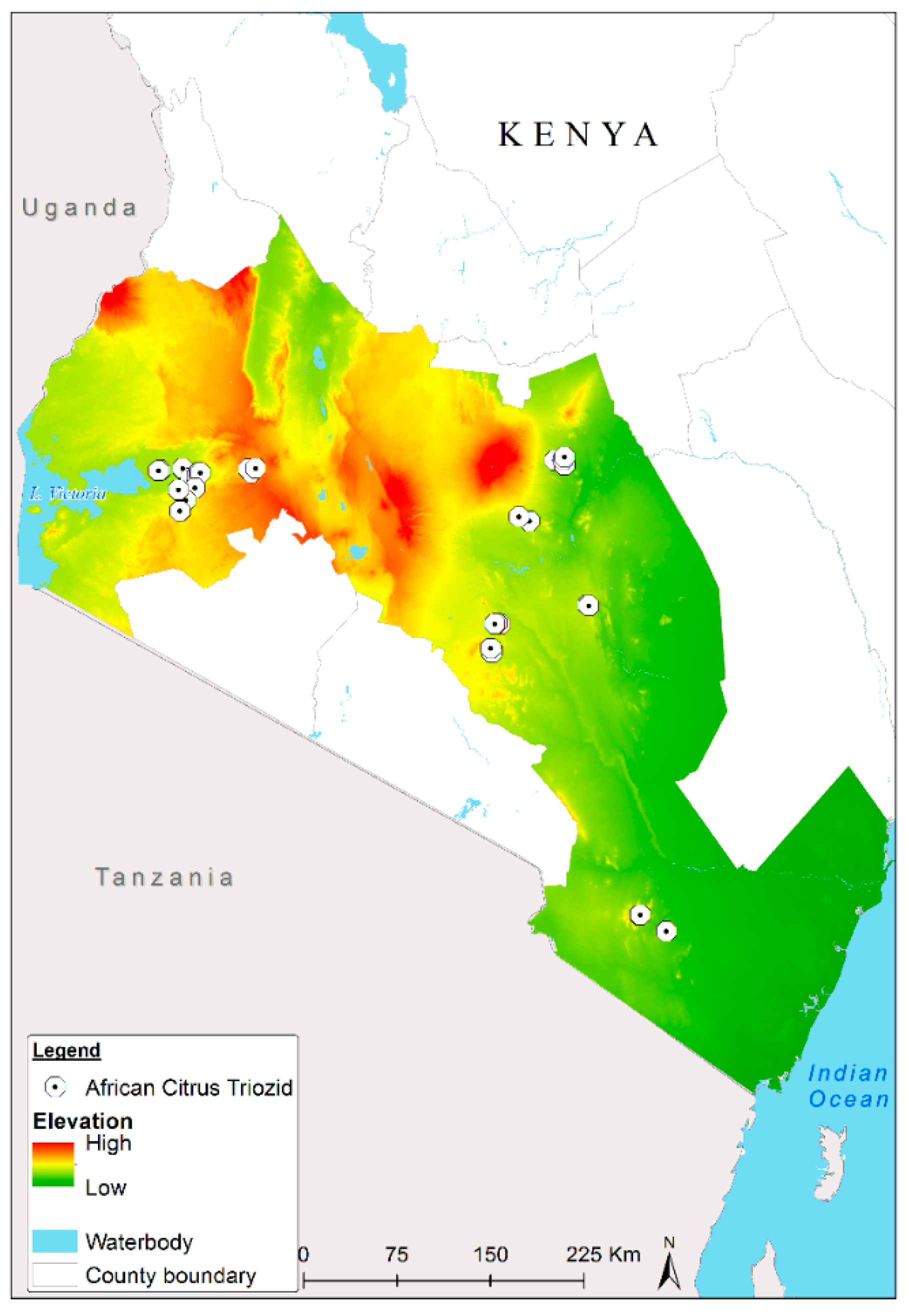
2.1. Study Area
2.2. ACT Occurrence Data
2.3. Predictor Variables
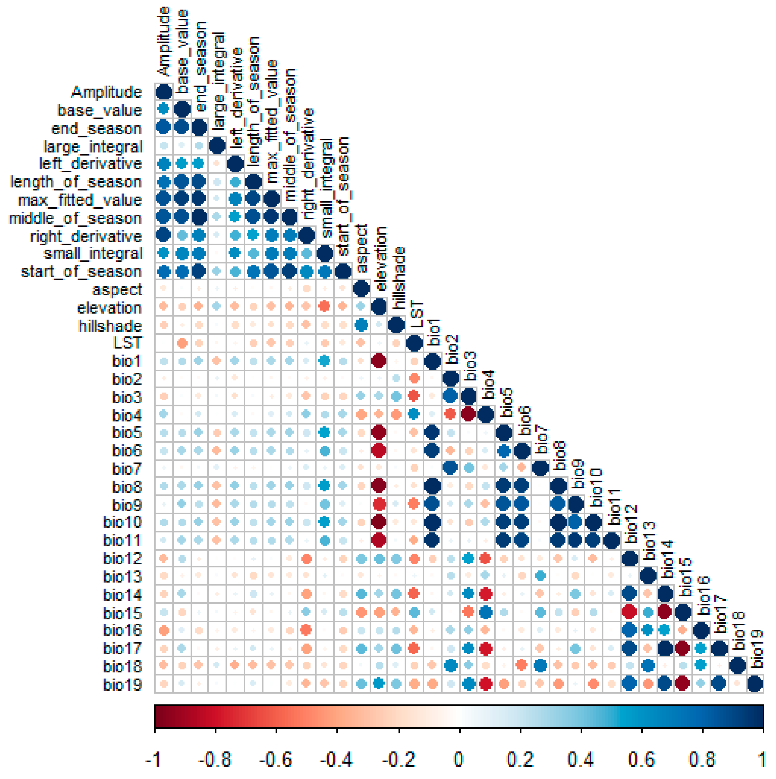
2.4. Predictor Variable Selection
2.5. EN Modeling
2.6. EN Models Validation
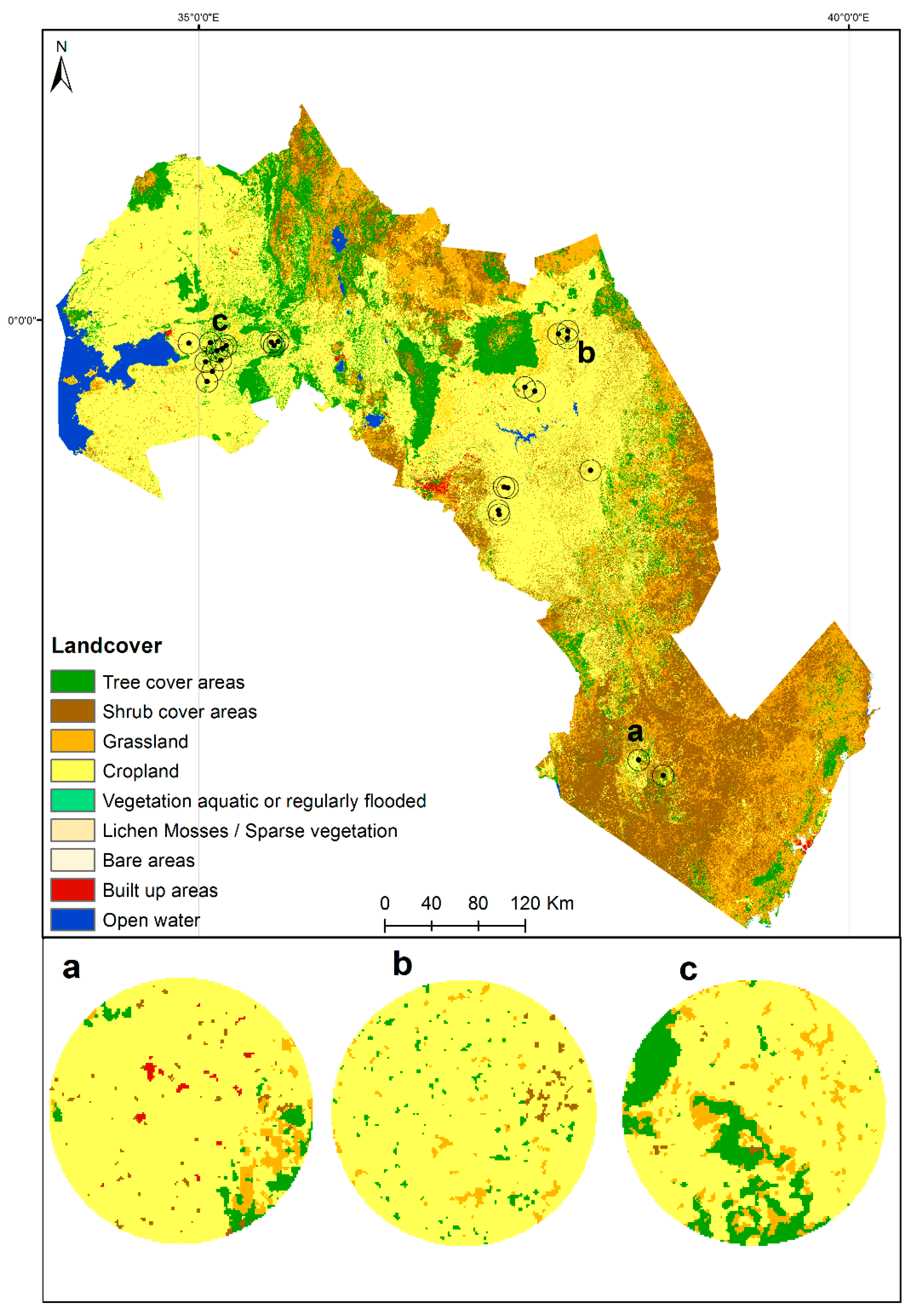
2.7. Landscape Context Calculation
3. Results
3.1. EN Models
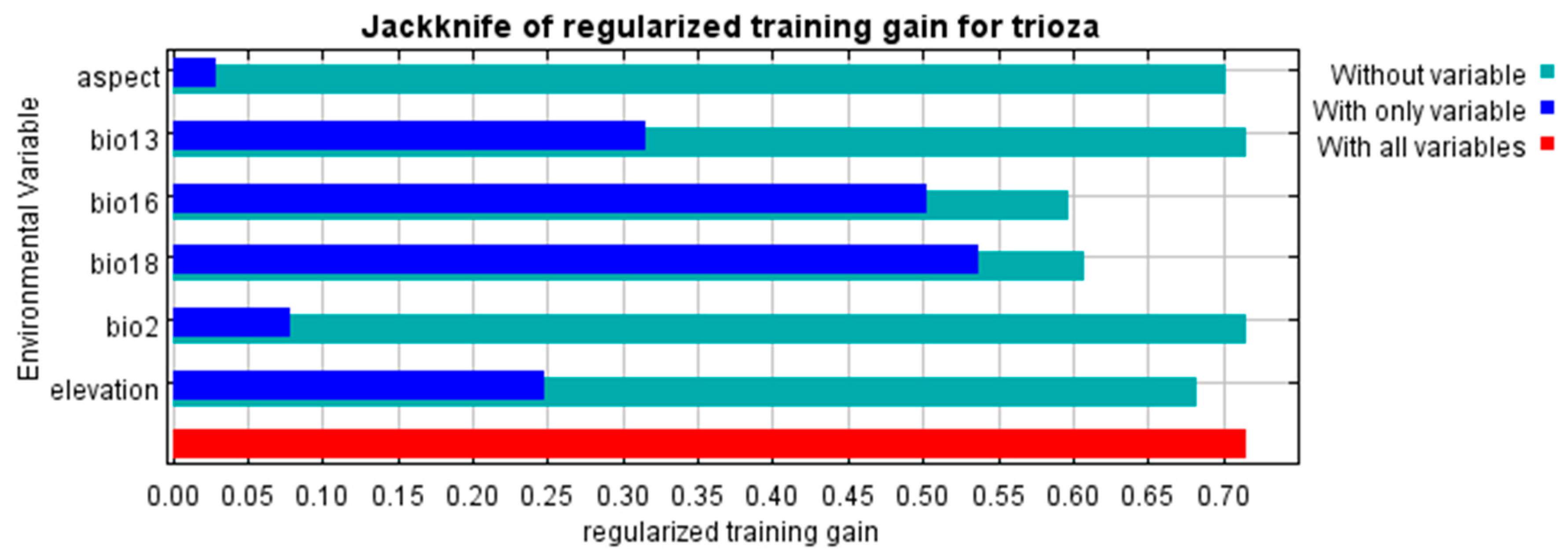
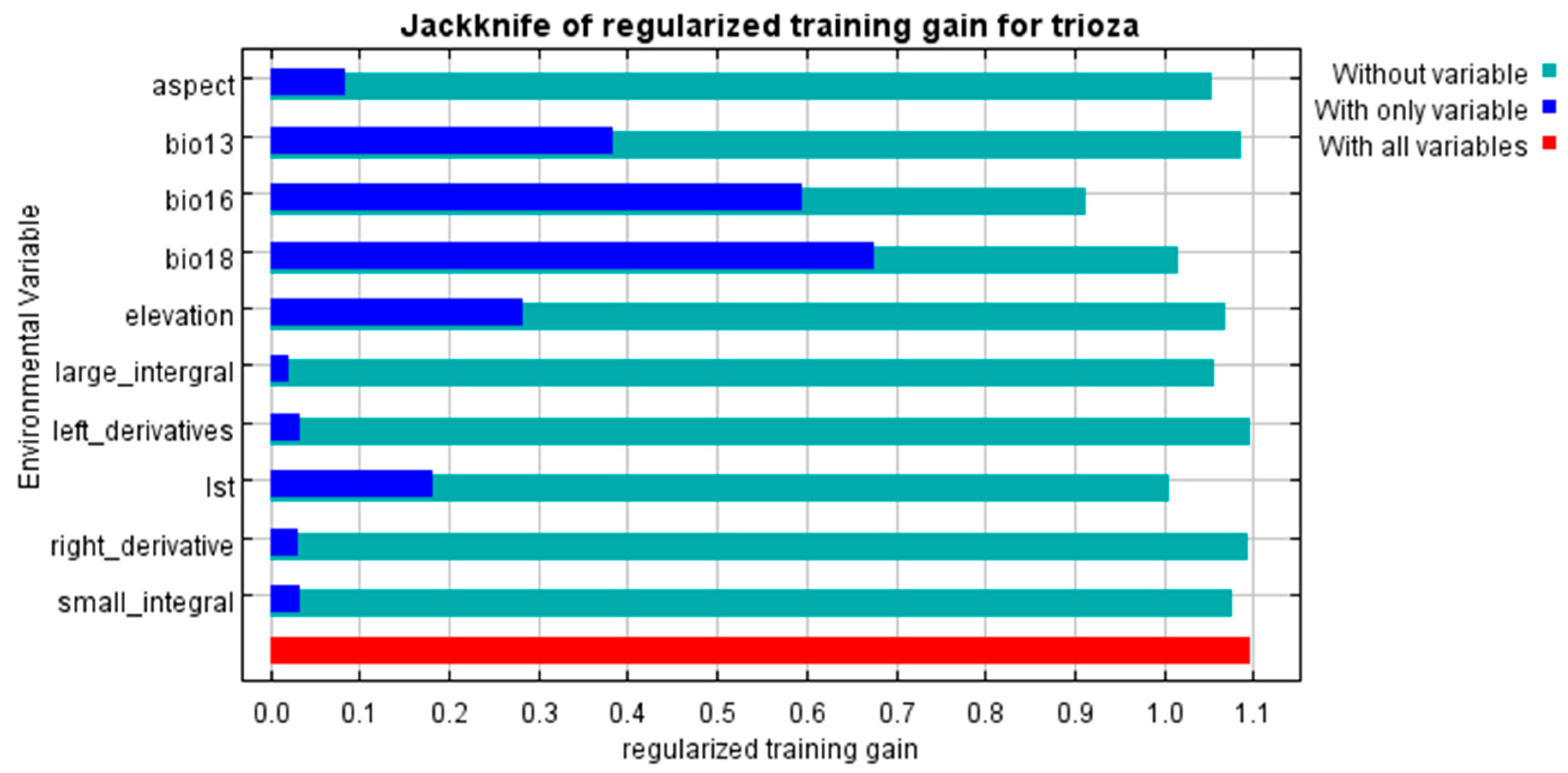
3.2. Variable Importance
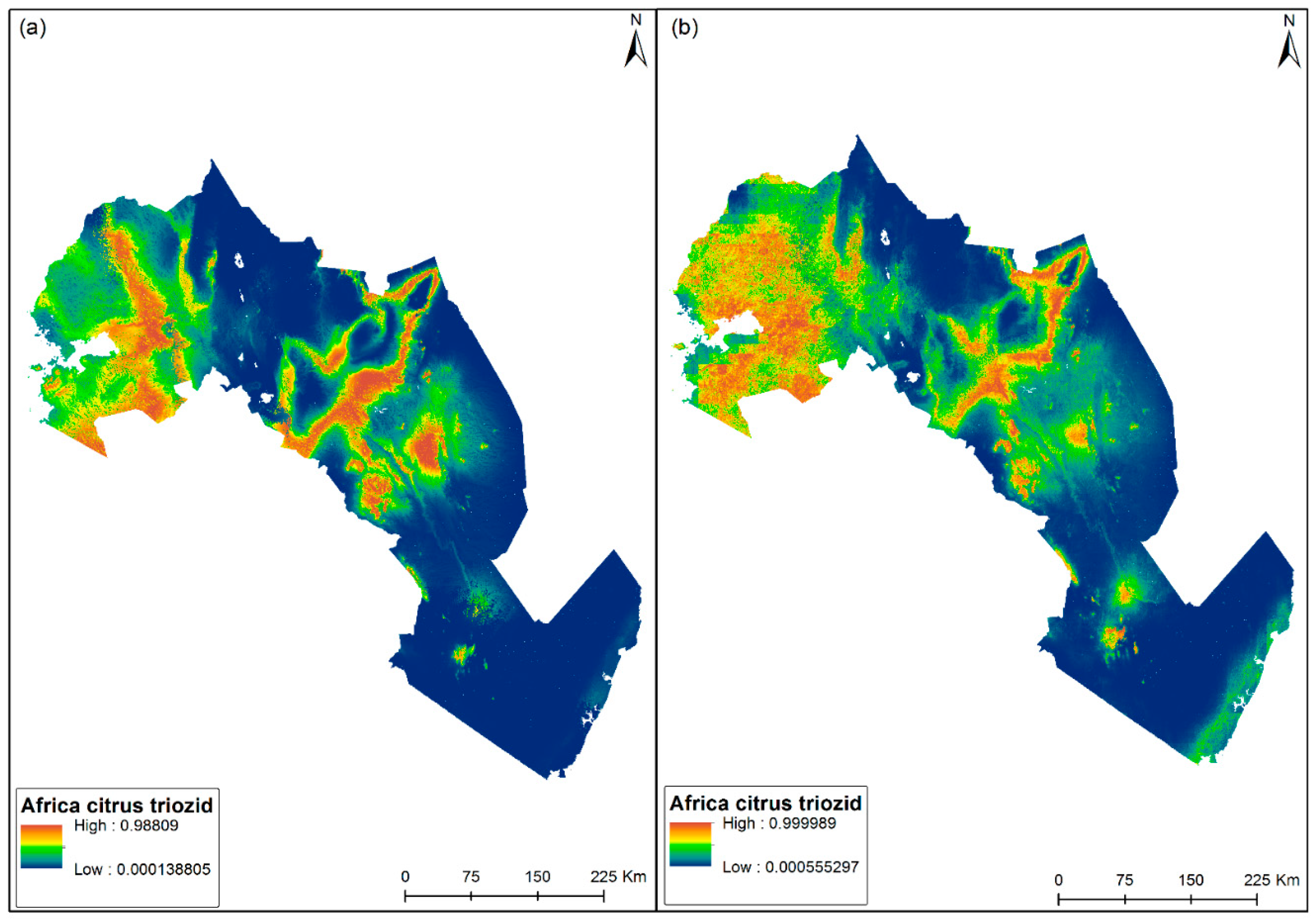
3.3. Habitat Suitability Mapping
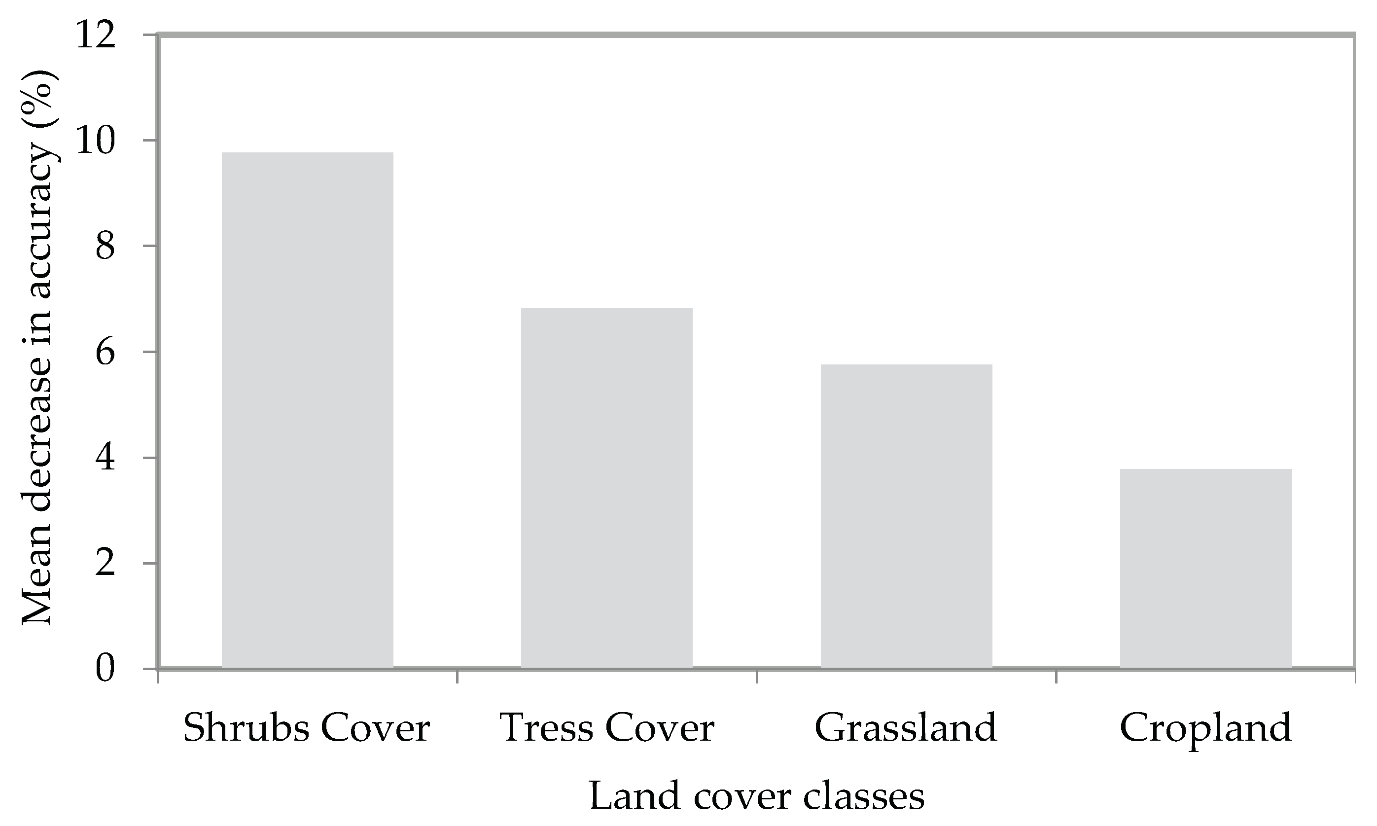
3.4. Relationship between ACT Habitat Suitability and Landscape Context
4. Discussion
5. Conclusions
Author Contributions
Funding
Acknowledgments
Conflicts of Interest
References
- Franco-Vega, A.; Reyes-Jurado, F.; Cardoso-Ugarte, G.A.; Sosa-Morales, M.E.; Palou, E.; López, M. Chapter 89—Sweet Orange (Citrus sinensis) Oils A2. In Essential Oils in Food Preservation, Flavor and Safety; Preedy, V.R., Ed.; Academic Press: San Diego, CA, USA, 2016; pp. 783–790. [Google Scholar]
- Liu, Y.; Heying, E.; Tanumihardjo, S.A. History, Global Distribution, and Nutritional Importance of Citrus Fruits. Compr. Rev. Food Sci. Food Saf. 2012, 11, 530–545. [Google Scholar] [CrossRef] [Green Version]
- FAO, Food and Agriculture Organization of the United. FAOSTAT Statistics Database; FAO: Rome, Italy, 2016. [Google Scholar]
- Ouma, G. Challenges and approaches to sustainable citrus production in Kenya. Afr. J. Plant Sci. Biotechnol. 2008, 2, 49–51. [Google Scholar]
- Adhikari, U.; Nejadhashemi, A.P.; Woznicki, S.A. Climate change and eastern Africa: A review of impact on major crops. Food Energy Secur. 2015, 4, 110–132. [Google Scholar] [CrossRef]
- Nicholas, I.D. 26—Plantings in Tropical and Subtropical Areas A2. In Windbreak Technology; Brandle, J.R., Hintz, D.L., Sturrock, J.W., Eds.; Elsevier: Amsterdam, The Netherlands, 1988; pp. 465–482. [Google Scholar]
- Asharaf, S.; Khan, A.G.; Ali, S.; Iftikhar, M. An Assessment of the Socio-Economic Factors Affecting the Adoption of Citrus Tissue Culture Technology in Kenya; Ciencia Rural: Santa Maria, Brazil, 2002. [Google Scholar]
- Waithaka, K. Consultant’s Report on Tropical Fruit Production in East and Southern Africa; Food and Agriculture Organization of the United Nations: Rome, Italy, 1991. [Google Scholar]
- ICIPE. SCIPM: Project by ICIPE and Partners to Improve Citrus Farming. 2015. Available online: http://www.icipe.org/news/scipm-project-icipe-and-partners-improve-citrus-farming (accessed on 17 April 2018).
- Michaud, J.P. Natural mortality of Asian citrus psyllid (Homoptera: Psyllidae) in Central Florida. Biol. Control 2004, 29, 260–269. [Google Scholar] [CrossRef]
- Zou, H.; Gowda, S.; Zhou, L.; Hajeri, S.; Chen, G.; Duan, Y. The Destructive Citrus Pathogen, ‘Candidatus Liberibacter asiaticus’ Encodes a Functional Flagellin Characteristic of a Pathogen-Associated Molecular Pattern. PLoS ONE 2012, 7, e46447. [Google Scholar] [CrossRef] [PubMed]
- Boykin, L.M.; De Barro, P.; Hall, D.G.; Hunter, W.B.; McKenzie, C.L.; Powell, C.A.; Shatters, R.G. Overview of worldwide diversity of Diaphorina citri Kuwayama mitochondrial cytochrome oxidase 1 haplotypes: Two Old World lineages and a New World invasion. Bull. Entomol. Res. 2012, 102, 573–582. [Google Scholar] [CrossRef] [PubMed]
- Jagoueix, S.; Bove, M.J.; Garnier, M. The phloem-limited bacterium of greening disease of citrus is a member of the α subdivision of the proteobacteria. Int. J. Syst. Bacteriol. 1994, 44, 379–386. [Google Scholar] [CrossRef] [PubMed]
- Khamis, F.M.; Rwomushana, I.; Ombura, L.O.; Cook, G.; Tanga, C.M.; Ekesi, S. DNA Barcode Reference Library for the African Citrus Triozid, Trioza erytreae (Hemiptera: Triozidae): Vector of African Citrus Greening. J. Econ. Entomol. 2017, 110, 2637–2646. [Google Scholar] [CrossRef] [PubMed]
- Catling, H.D. Notes on the biology of the South African citrus psylla, Trioza erytreae (Del Guercio) (Homoptera: Psyllidae). J. Entomol. Soc. S. Afr. 1973, 36, 299–306. [Google Scholar]
- Aubert, B. Trioza erytreae Del Guercio and Diaphorina citri Kuwayama (Homoptera: Psyllidae), the two vectors of citrus greening disease: Biological aspects and possible control strategies. Fruits 1987, 42, 149–162. [Google Scholar]
- Dormann, C.F.; Elith, J.; Bacher, S.; Buchmann, C.; Carl, G.; Carré, G.; Marquéz, J.R.G.; Gruber, B.; Lafourcade, B.; Leitão, P.J.; et al. Collinearity: A review of methods to deal with it and a simulation study evaluating their performance. Ecography 2013, 36, 27–46. [Google Scholar] [CrossRef]
- Pole, F.N.; Ndung’u, J.M.; Kimani, J.M. Citrus farming in Kwale district: A case study of Lukore location. In Proceedings of the 12th KARI Biennial Conference: Transforming Agriculture for Improved Livelihoods through Agricultural Product Value Chains, Nairobi, Kenya, 8–12 November 2010. [Google Scholar]
- Alvarez, S.; Rohrig, E.; Solís, D.; Thomas, M.H. Citrus Greening Disease (Huanglongbing) in Florida: Economic Impact, Management and the Potential for Biological Control. Agric. Res. 2016, 5, 109–118. [Google Scholar] [CrossRef]
- Grafton-Cardwell, E.E.; Stelinski, L.L.; Stansly, P.A. Biology and Management of Asian Citrus Psyllid, Vector of the Huanglongbing Pathogens. Annu. Rev. Entomol. 2013, 58, 413–432. [Google Scholar] [CrossRef] [PubMed]
- Moore, S.M.; Borer, E.T.; Hosseini, P.R. Predators indirectly control vector-borne disease: Linking predator–prey and host–pathogen models. J. R. Soc. Interface 2010, 7, 161–176. [Google Scholar] [CrossRef] [PubMed]
- Peterson, A.T. Ecologic Niche Modeling and Spatial Patterns of Disease Transmission. Emerg. Infect. Dis. 2006, 12, 1822–1826. [Google Scholar] [CrossRef] [PubMed] [Green Version]
- Brownstein, J.S.; Holford, T.R.; Fish, D. A climate-based model predicts the spatial distribution of the Lyme disease vector Ixodes scapularis in the United States. Environ. Health Perspect. 2003, 111, 1152–1157. [Google Scholar] [CrossRef] [PubMed]
- Lord, C.C. Modeling and biological control of mosquitoes. J. Am. Mosq. Control Assoc. 2007, 23, 252–264. [Google Scholar] [CrossRef]
- Hol, W.H.; Bezemer, T.M.; Biere, A. Getting the ecology into interactions between plants and the plant growth-promoting bacterium Pseudomonas fluorescens. Front. Plant Sci. 2013, 4, 81. [Google Scholar] [CrossRef] [PubMed]
- Shabani, F.; Kumar, L.; Ahmadi, M. A comparison of absolute performance of different correlative and mechanistic species distribution models in an independent area. Ecol. Evol. 2016, 6, 5973–5986. [Google Scholar] [CrossRef] [PubMed] [Green Version]
- Yackulic, C.B.; Chandler, R.; Zipkin, E.F.; Royle, J.A.; Nichols, J.D.; Campbell Grant, E.H.; Veran, S. Presence-only modelling using MAXENT: When can we trust the inferences? Methods Ecol. Evol. 2013, 4, 236–243. [Google Scholar] [CrossRef]
- Zhu, Z.; Woodcock, C.E. Potential Geographic Distribution of Brown Marmorated Stink Bug Invasion (Halyomorpha halys). PLoS ONE 2012, 7, e31246. [Google Scholar] [CrossRef] [PubMed]
- Barredo, J.I.; Strona, G.; Rigo, D.; Caudullo, G.; Stancanelli, G.; San-Miguel-Ayanz, J. Assessing the potential distribution of insect pests: Case studies on large pine weevil (Hylobius abietis L) and horse-chestnut leaf miner (Cameraria ohridella) under present and future climate conditions in European forests. EPPO Bull. 2015, 45, 273–281. [Google Scholar] [CrossRef]
- Hof, A.R.; Svahlin, A. The potential effect of climate change on the geographical distribution of insect pest species in the Swedish boreal forest. Scand. J. For. Res. 2016, 31, 29–39. [Google Scholar] [CrossRef]
- Marchioro, C.A. Global Potential Distribution of Bactrocera carambolae and the Risks for Fruit Production in Brazil. PLoS ONE 2016, 11, e0166142. [Google Scholar] [CrossRef] [PubMed]
- Alkishe, A.A.; Peterson, A.T.; Samy, A.M. Climate change influences on the potential geographic distribution of the disease vector tick Ixodes ricinus. PLoS ONE 2017, 12, e0189092. [Google Scholar] [CrossRef] [PubMed]
- Chiyaka, C.; Singer, B.H.; Halbert, S.E.; Morris, J.G.; van Bruggen, A.H.C. Modeling huanglongbing transmission within a citrus tree. Proc. Natl. Acad. Sci. USA 2012, 109, 12213–12218. [Google Scholar] [CrossRef] [PubMed] [Green Version]
- Vilamiu, R.G.d.A.; Ternes, S.; Braga, G.A.; Laranjeira, F.F. A model for Huanglongbing spread between citrus plants including delay times and human intervention. Proc. Natl. Acad. Sci. USA 2012, 1479, 2315–2319. [Google Scholar]
- Ramirez, G.R.G.; Medina, H.C.P.B.; Trujillo, T.J.R. Agroclimatic risk of development of Diaphorina citri in the citrus region of Nuevo Leon, Mexico. Afr. J. Agric. Res. 2016, 11, 3254–3260. [Google Scholar]
- Shimwela, M.M.; Narouei-Khandan, H.A.; Halbert, S.E.; Keremane, M.L.; Minsavage, G.V.; Timilsina, S.; Massawe, D.P.; Jones, J.B.; van Bruggen, A.H.C. First occurrence of Diaphorina citri in East Africa, characterization of the Ca. Liberibacter species causing huanglongbing (HLB) in Tanzania, and potential further spread of D. citri and HLB in Africa and Europe. Eur. J. Plant Pathol. 2016, 146, 349–368. [Google Scholar] [CrossRef]
- Narouei-Khandan, H.A.; Halbert, S.E.; Worner, S.P.; van Bruggen, A.H.C. Global climate suitability of citrus huanglongbing and its vector, the Asian citrus psyllid, using two correlative species distribution modeling approaches, with emphasis on the USA. Eur. J. Plant Pathol. 2016, 144, 655–670. [Google Scholar] [CrossRef]
- Paull, S.H.; Song, S.; McClure, K.M.; Sackett, L.C.; Kilpatrick, A.M.; Johnson, P.T.J. From superspreaders to disease hotspots: Linking transmission across hosts and space. Front. Ecol. Environ. 2012, 10, 75–82. [Google Scholar] [CrossRef] [PubMed]
- Zimmermann, N.E.; Edwards, T.C., Jr.; Moisen, G.G.; Frescino, T.S.; Blackard, J.A. Remote sensing-based predictors improve distribution models of rare, early successional and broadleaf tree species in Utah. J. Appl. Ecol. 2007, 44, 1057–1067. [Google Scholar] [CrossRef] [PubMed]
- Green, G.C.; Catling, H.D. Weather induced mortality of the citrus psylla, trioza erytreae (del guercio) (homoptera: Psyllidae), a vector of greening virus, in some citrus producing areas of Southern Africa. Agric. Meteorol. 1971, 8, 305–317. [Google Scholar] [CrossRef]
- Amoros Lopez, J. Land cover classification of VHR airborne images for citrus grove identification. ISPRS J. Photogramm. Remote Sens. 2011, 66, 115–123. [Google Scholar] [CrossRef]
- Ozdemir, L. Separation of Citrus Plantations from forest cover using Landsat Imagery. Allg. For. Jagdztg. 2007, 178, 208–212. [Google Scholar]
- Shrivastava, R.J.; Gebelein, J.L. Landcover classification and economic assessment of citrus groves using remote sensing. ISPRS J. Photogramm. Remote Sens. 2007, 61, 341–353. [Google Scholar] [CrossRef]
- Plantegenest, M.; Le May, C.; Fabre, F.D.R. Landscape epidemiology of plant diseases. J. R. Soc. Interface 2007, 4, 963–972. [Google Scholar] [CrossRef] [PubMed] [Green Version]
- Margosian, M.L.; Garrett, K.A.; Hutchinson, J.M.S.; With, K.A. Connectivity of the American Agricultural Landscape: Assessing the National Risk of Crop Pest and Disease Spread. BioSci 2009, 59, 141–151. [Google Scholar] [CrossRef] [Green Version]
- Rizzo, D.M.; Garbelotto, M. Sudden oak death: Endangering California and Oregon forest ecosystems. Front. Ecol. Environ. 2003, 1, 197–204. [Google Scholar] [CrossRef]
- Avelino, J.; Romero-Gurdian, A.; Cruz-Cuellar, H.F.; Declerck, F.A. Landscape context and scale differentially impact coffee leaf rust, coffee berry borer, and coffee root-knot nematodes. Ecol. Appl. 2012, 22, 584–596. [Google Scholar] [CrossRef] [PubMed]
- Thies, C.; Steffan-Dewenter, I.; Tscharntke, T. Effects of landscape context on herbivory and parasitism at different spatial scales. Oikos 2003, 101, 18–25. [Google Scholar] [CrossRef] [Green Version]
- Oosten, C.V. Farming Systems and Food Security in Kwale District Kenya; MOPAN Development, Ed.; Africa Studies Centre: Leiden, The Netherlands, 1989. [Google Scholar]
- Anonymous. Horticulture Crops Protection Handbook; Ministry of Agriculture: Nairobi, Kenya, 1984.
- Wisz, M.S.; Hijmans, R.J.; Li, J.; Peterson, A.T.; Graham, C.H.; Guisan, A. Effects of sample size on the performance of species distribution model. Divers. Distrib. 2008, 14, 763–773. [Google Scholar] [CrossRef]
- Amirpour Haredasht, S.; Barrios, M.; Farifteh, J.; Maes, P.; Clement, J.; Verstraeten, W.W.; Tersago, K.; Van Ranst, M.; Coppin, P.; Berckmans, D.; et al. Ecological niche modelling of bank voles in Western Europe. Int. J. Environ. Res. Public Health 2013, 10, 499–514. [Google Scholar] [CrossRef] [PubMed]
- Qin, A.; Liu, B.; Guo, Q.; Bussmann, R.W.; Ma, F.; Jian, Z.; Xu, G.; Pei, S. Maxent modeling for predicting impacts of climate change on the potential distribution of Thuja sutchuenensis Franch., an extremely endangered conifer from southwestern China. Glob. Ecol. Conserv. 2017, 10, 139–146. [Google Scholar] [CrossRef]
- Hijmans, R.J.; Cameron, S.E.; Parra, J.L.; Jones, P.G.; Jarvis, A. Very high resolution interpolated climate surfaces for global land areas. Int. J. Climatol. 2005, 25, 1965–1978. [Google Scholar] [CrossRef] [Green Version]
- Pierce, K.B.; Lookingbill, T.; Urban, D. Urban, A simple method for estimating potential relative radiation (PRR) for landscape-scale vegetation analysis. Landscape Ecology. Landsc. Ecol. 2005, 20, 137–147. [Google Scholar] [CrossRef]
- Jarvis, A.; Reuter, H.I.; Nelson, A.; Guevara, E. Hole-Filled SRTM for the Globe Version 4. The CGIAR Consortium for Spatial Information (CGIAR-CSI). 2008. Available online: http://srtm.csi.cgiar.org/ (accessed on 16 May 2018).
- Usery, E.L.; Finn, M.P.; Scheidt, D.J.; Ruhl, S.; Beard, T.; Bearden, M. Geospatial data resampling and resolution effects on watershed modeling: A case study using the agricultural non-point source pollution model. J. Geogr. Syst. 2004, 6, 289–306. [Google Scholar] [CrossRef]
- Li, Z.; Li, X.; Wei, D.; Xu, X.; Wang, H. An assessment of correlation on MODIS-NDVI and EVI with natural vegetation coverage in Northern Hebei Province, China. Procedia Environ. Sci. 2010, 2, 964–969. [Google Scholar] [CrossRef]
- Matsushita, B.; Yang, W.; Chen, J.; Onda, Y.; Qiu, G. Sensitivity of the Enhanced Vegetation Index (EVI) and Normalized Difference Vegetation Index (NDVI) to Topographic Effects: A Case Study in High-Density Cypress Forest. Sensors 2007, 7, 2636–2651. [Google Scholar] [CrossRef] [PubMed]
- Wang, Z.; Liu, C.; Chen, W.; Lin, X. Preliminary Comparison of MODIS-NDVI and MODIS-EVI in Eastern Asia; Geomatics and Information Science of Wuhan University: Wuhan, China, 2006; Volume 31, pp. 407–410. [Google Scholar]
- Liu, S.; Liu, X.; Liu, M.; Wu, L.; Ding, C.; Huang, Z. Extraction of Rice Phenological Differences under Heavy Metal Stress Using EVI Time-Series from HJ-1A/B Data. Sensors 2017, 17, 1243. [Google Scholar] [CrossRef]
- Huete, A.; Didan, K.; Miura, T.; Rodriguez, E.; Gao, X.; Ferreira, L.G. Overview of the Radiometric and Biophysical Performance of the MODIS Vegetation Indices. Remote Sens. Environ. 2002, 83, 195–213. [Google Scholar] [CrossRef]
- Tuck, S.L.; Phillips, H.R.P.; Hintzen, R.E.; Scharlemann, J.P.W.; Purvis, A.; Hudson, L.N. MODISTools—Downloading and processing MODIS remotely sensed data in R. Ecol. Evol. 2014, 4, 4658–4668. [Google Scholar] [CrossRef] [PubMed]
- Jönsson, P.; Eklundh, L. TIMESAT—A program for analyzing time-series of satellite sensor data. Comput. Geosci. 2004, 30, 833–845. [Google Scholar] [CrossRef]
- Wei, H.; Heilman, P.; Qi, J.; Nearing, M.A.; Gu, Z.; Zhang, Y. Assessing phenological change in China from 1982 to 2006 using AVHRR imagery. Front. Earth Sci. 2012, 6, 227–236. [Google Scholar] [CrossRef]
- Penatti, N.; Isnard, T. Subdivision of pantanal quaternary wetlands: Modis NDVI timeseries in the indirect detection of sediments granulometry. Int. Arch. Photogramm. Remote Sens. Spat. Inf. Sci. 2012, XXXIX-B8, 311–316. [Google Scholar] [CrossRef]
- Cai, Z.; Jönsson, P.; Jin, H.; Eklundh, L. Performance of Smoothing Methods for Reconstructing NDVI Time-Series and Estimating Vegetation Phenology from MODIS Data. Remote Sens. 2017, 9, 1271. [Google Scholar] [CrossRef]
- Chen, J. A simple method for reconstructing a high-quality NDVI time-series data set based on the Savitzky-Golay filter. Remote Sens. Environ. 2004, 91, 332–344. [Google Scholar] [CrossRef]
- Makori, D.; Fombong, A.; Abdel-Rahman, E.; Nkoba, K.; Ongus, J.; Irungu, J.; Mosomtai, G.; Makau, S.; Mutanga, O.; Odindi, J.; et al. Predicting Spatial Distribution of Key Honeybee Pests in Kenya Using Remotely Sensed and Bioclimatic Variables: Key Honeybee Pests Distribution Models. ISPRS Int. J. Geo-Inf. 2017, 6, 66. [Google Scholar] [CrossRef]
- Chabot-Couture, G.; Nigmatulina, K.; Eckhoff, P. An Environmental Data Set for Vector-Borne Disease Modeling and Epidemiology. PLoS ONE 2014, 9, e94741. [Google Scholar] [CrossRef] [PubMed]
- Phillips, S.J.; Anderson, R.P.; Schapire, R.E. Maximum entropy modeling of species geographic distributions. Ecol. Model. 2006, 190, 231–259. [Google Scholar] [CrossRef]
- Buermann, W.; Saatchi, S.; Smith, T.B.; Zutta, B.R.; Chaves, J.A.; Milá, B.; Graham, C.H. Predicting species distributions across the Amazonian and Andean regions using remote sensing data. J. Biogeogr. 2008, 35, 1160–1176. [Google Scholar] [CrossRef]
- Royle, J.A.; Chandler, R.B.; Yackulic, C.; Nichols, J.D. Likelihood analysis of species occurrence probability from presence-only data for modelling species distributions. Methods Ecol. Evol. 2012, 3, 545–554. [Google Scholar] [CrossRef]
- Sahlean, T.C.; Gherghel, I.; Papeş, M.; Strugariu, A.; Zamfirescu, Ş.R. Refining Climate Change Projections for Organisms with Low Dispersal Abilities: A Case Study of the Caspian Whip Snake. PLoS ONE 2014, 9, e91994. [Google Scholar] [CrossRef] [PubMed]
- Cord, A.F.; Klein, D.; Gernandt, D.S.; de la Rosa, J.A.P.; Dech, S. Remote sensing data can improve predictions of species richness by stacked species distribution models: A case study for Mexican pines. J. Biogeogr. 2014, 41, 736–748. [Google Scholar] [CrossRef]
- Anderson, R.P.; Lew, D.; Peterson, A.T. Evaluating predictive models of species’ distributions: Criteria for selecting optimal models. Ecol. Model. 2003, 162, 211–232. [Google Scholar] [CrossRef]
- Jorge Soberon, B. Mapping Species Distributions: Spatial Inference and Prediction. Q. Rev. Biol. 2011, 86, 219–220. [Google Scholar]
- Allouche, O.; Tsoar, A.; Kadmon, R. Assessing the accuracy of species distribution models: Prevalence, kappa and the true skill statistic (TSS). J. Appl. Ecol. 2006, 43, 1223–1232. [Google Scholar] [CrossRef]
- Zhang, L.; Liu, S.; Sun, P.; Wang, T.; Wang, G.; Zhang, X.; Wang, L. Consensus Forecasting of Species Distributions: The Effects of Niche Model Performance and Niche Properties. PLoS ONE 2015, 10, e0120056. [Google Scholar] [CrossRef] [PubMed]
- Matyukhina, D.S.; Miquelle, D.G.; Murzin, A.A.; Pikunov, D.G.; Fomenko, P.V.; Aramilev, V.V.; Litvinov, M.N.; Salkina, G.P.; Seryodkin, I.V.; Nikolaev, I.G.; et al. Assessing the Influence of Environmental Parameters on Amur Tiger Distribution in the Russian Far East Using a MaxEnt Modeling Approach. Achiev. Life Sci. 2014, 8, 95–100. [Google Scholar] [CrossRef]
- ESA CCI Land Cover-S2 Prototype Land Cover Map of Africa. Available online: http://www.2016africalandcover20m.esrin.esa.int/ (accessed on 23 May 2018).
- Van Den Berg, M.A.; Anderson, S.H.; Deacon, V.E. Population studies of the citrus psylla, trioza erytreae: Factors influencing dispersal. Phytoparasitica 1991, 19, 283. [Google Scholar] [CrossRef]
- Breiman, L. Random Forests. Mach. Learn. 2001, 45, 5–32. [Google Scholar] [CrossRef] [Green Version]
- Wang, L.; Zhou, X.; Zhu, X.; Dong, Z.; Guo, W. Estimation of biomass in wheat using random forest regression algorithm and remote sensing data. Crop J. 2016, 4, 212–219. [Google Scholar] [CrossRef]
- Forkuor, G.; Hounkpatin, O.K.L.; Welp, G.; Thiel, M. High Resolution Mapping of Soil Properties Using Remote Sensing Variables in South-Western Burkina Faso: A Comparison of Machine Learning and Multiple Linear Regression Models. PLoS ONE 2017, 12, e0170478. [Google Scholar] [CrossRef] [PubMed]
- Tonnang, H.E.Z.; Hervé, B.D.B.; Biber-Freudenberger, L.; Salifu, D.; Subramanian, S.; Ngowi, V.B.; Guimapi, R.Y.A.; Anani, B.; Kakmeni, F.M.M.; Affognon, H.; et al. Advances in crop insect modelling methods—Towards a whole system approach. Ecol. Model. 2017, 354, 88–103. [Google Scholar] [CrossRef]
- De Meyer, M.; Robertson, M.P.; Mansell, M.W.; Ekesi, S.; Tsuruta, K.; Mwaiko, W.; Vayssieres, J.F.; Peterson, A.T. Ecological niche and potential geographic distribution of the invasive fruit fly Bactrocera invadens (Diptera, Tephritidae). Bull. Entomol. Res. 2010, 100, 35–48. [Google Scholar] [CrossRef] [PubMed]
- Bové, J.M. Huanglongbing or yellow shoot, a disease of Gondwanan origin: Will it destroy citrus worldwide? Phytoparasitica 2014, 42, 579–583. [Google Scholar] [CrossRef] [Green Version]
- Blum, M.; Lensky, I.M.; Rempoulakis, P.; Nestel, D. Modeling insect population fluctuations with satellite land surface temperature. Ecol. Model. 2015, 311, 39–47. [Google Scholar] [CrossRef]
- Ratnadass, A.; Fernandes, P.; Avelino, J.; Habib, R. Plant species diversity for sustainable management of crop pests and diseases in agroecosystems: Review. Agron. Sustain. Dev. 2012, 32, 273–303. [Google Scholar] [CrossRef] [Green Version]
- Cook, G.; Maqutu, V.Z.; Vuuren, S.P.V. Population Dynamics and Seasonal Fluctuation in the Percentage infection of Trioza erytreae with ‘Candidatus’ Liberibacter Africanus, the African Citrus Greening Pathogen, in an Orchard Severely Infected with African Greening and Transmission by Field-Collected Trioza erytreae. Afr. Entomol. 2013, 22, 127–135. [Google Scholar]


| Data Source | Category | Variables Description | Abbreviations | Units |
|---|---|---|---|---|
| WorldClim | Bioclimatic | Annual mean temperature | Bio 1 | °C |
| Mean diurnal range (mean of monthly (max temp, min temp)) | Bio 2 | °C | ||
| Isothermality (Bio 2/Bio 7) (×100) | Bio 3 | °C | ||
| Temperature seasonality (standard deviation × 100) | Bio 4 | °C | ||
| Maximum temperature of warmest month | Bio 5 | °C | ||
| Minimum temperature of coldest month | Bio 6 | °C | ||
| Temperature annual range (Bio 5-Bio 6) | Bio 7 | °C | ||
| Mean temperature of wettest quarter | Bio 8 | °C | ||
| Mean temperature of driest quarter | Bio 9 | °C | ||
| Mean temperature of warmest quarter | Bio 11 | °C | ||
| Mean temperature of coldest quarter | Bio 11 | °C | ||
| Annual precipitation | Bio 12 | mm | ||
| Precipitation of wettest month | Bio 13 | mm | ||
| Precipitation of driest month | Bio 14 | mm | ||
| Precipitation seasonality (coefficient of variation) | Bio 15 | mm | ||
| Precipitation of wettest quarter | Bio 16 | mm | ||
| Precipitation of driest quarter | Bio 17 | mm | ||
| Precipitation of warmest quarter | Bio 18 | mm | ||
| Precipitation of coldest quarter | Bio19 | mm | ||
| SRTM | Topographic | Ground height | Elevation | m |
| Sloping direction | Aspect | degree | ||
| Steepness of the ground | Slope | degree | ||
| Shading effect | Hill shade | n/a | ||
| MODIS EVI | Remotely sensed | Time for the start of the season | Start of season | decades |
| Time for the end of season | End of season | decades | ||
| Length of season from start to end | Length of season | decades | ||
| Mid of the season | Mid of season | decades | ||
| Difference between maximum and base level | Amplitude | n/a | ||
| Average minimum EVI value | Base value | n/a | ||
| Maximum fitted value | Max fitted value | n/a | ||
| Rate of increase at the beginning of season | Left derivative | % | ||
| Rate of decrease at the end of season | Right derivative | % | ||
| Large seasonal integral | Large integral | n/a | ||
| Small seasonal integral | Small integral | n/a | ||
| MODIS | Land surface temperature | LST | °C |
| Model | Bio-Climatic and Topographical Variables (BCL, n = 6) | Bio-Climatic, Topographical and Remotely-Sensed Variables (BCL-RS, n = 12) |
|---|---|---|
| Overall accuracy | 0.85 | 0.92 |
| Sensitivity | 0.73 | 0.91 |
| Specificity | 0.85 | 0.92 |
| Khat | 0.30 | 0.42 |
| TSS | 0.57 | 0.83 |
| Variables | Percent Contribution | Permutation Importance |
|---|---|---|
| BCL Model | ||
| Bio 16 | 49.3 | 40.5 |
| Bio 18 | 44.5 | 38.9 |
| Elevation | 04.0 | 18.3 |
| Aspect | 02.2 | 02.3 |
| Bio 2 | 00.0 | 00.0 |
| Bio 13 | 00.0 | 00.0 |
| BCL-RS Model | ||
| Bio 16 | 41.0 | 30.6 |
| Bio 18 | 36.3 | 23.9 |
| Land surface temperature (LST) | 06.6 | 11.5 |
| Elevation | 05.3 | 07.0 |
| Aspect | 04.9 | 07.8 |
| Small integral | 02.8 | 03.9 |
| Large integral | 02.5 | 07.6 |
| Bio 13 | 00.5 | 04.2 |
| Right derivative | 00.2 | 03.4 |
| Left derivatives | 00.0 | 00.1 |
© 2018 by the authors. Licensee MDPI, Basel, Switzerland. This article is an open access article distributed under the terms and conditions of the Creative Commons Attribution (CC BY) license (http://creativecommons.org/licenses/by/4.0/).
Share and Cite
Richard, K.; Abdel-Rahman, E.M.; Mohamed, S.A.; Ekesi, S.; Borgemeister, C.; Landmann, T. Importance of Remotely-Sensed Vegetation Variables for Predicting the Spatial Distribution of African Citrus Triozid (Trioza erytreae) in Kenya. ISPRS Int. J. Geo-Inf. 2018, 7, 429. https://doi.org/10.3390/ijgi7110429
Richard K, Abdel-Rahman EM, Mohamed SA, Ekesi S, Borgemeister C, Landmann T. Importance of Remotely-Sensed Vegetation Variables for Predicting the Spatial Distribution of African Citrus Triozid (Trioza erytreae) in Kenya. ISPRS International Journal of Geo-Information. 2018; 7(11):429. https://doi.org/10.3390/ijgi7110429
Chicago/Turabian StyleRichard, Kyalo, Elfatih M. Abdel-Rahman, Samira A. Mohamed, Sunday Ekesi, Christian Borgemeister, and Tobias Landmann. 2018. "Importance of Remotely-Sensed Vegetation Variables for Predicting the Spatial Distribution of African Citrus Triozid (Trioza erytreae) in Kenya" ISPRS International Journal of Geo-Information 7, no. 11: 429. https://doi.org/10.3390/ijgi7110429