2.3. MLP-CA Model for the Spatial Allocation of Land Use
An MLP-CA model was developed independently by combining multi-layer perception (MLP) [
19] and cellular automaton (CA) [
20]. Based on the MLP-CA model, corresponding transformation rules and principles were superposed to achieve the spatial allocation of the land use structure.
The MLP-CA model contains two modules, a training module and a simulation module. The training module is primarily realized by MLP and the simulation module is realized under the assistance of CA. The main process involves the automatic acquisition of internal transformation rules using training data in the training module; then, the external transformation rule is superposed. Later, these transformation rules are input to the simulation module to complete land use allocation [
21]. The detailed process is described below.
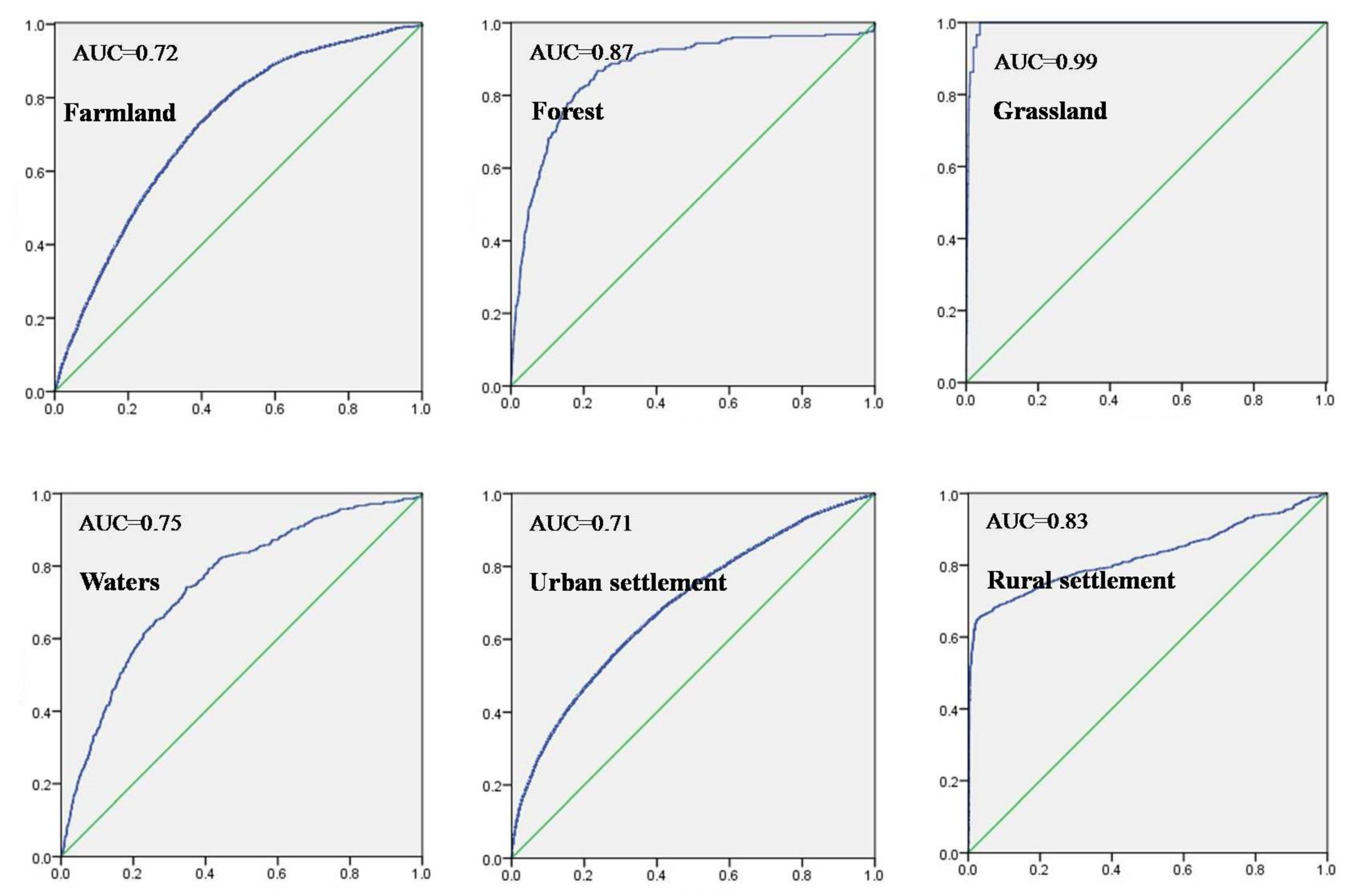
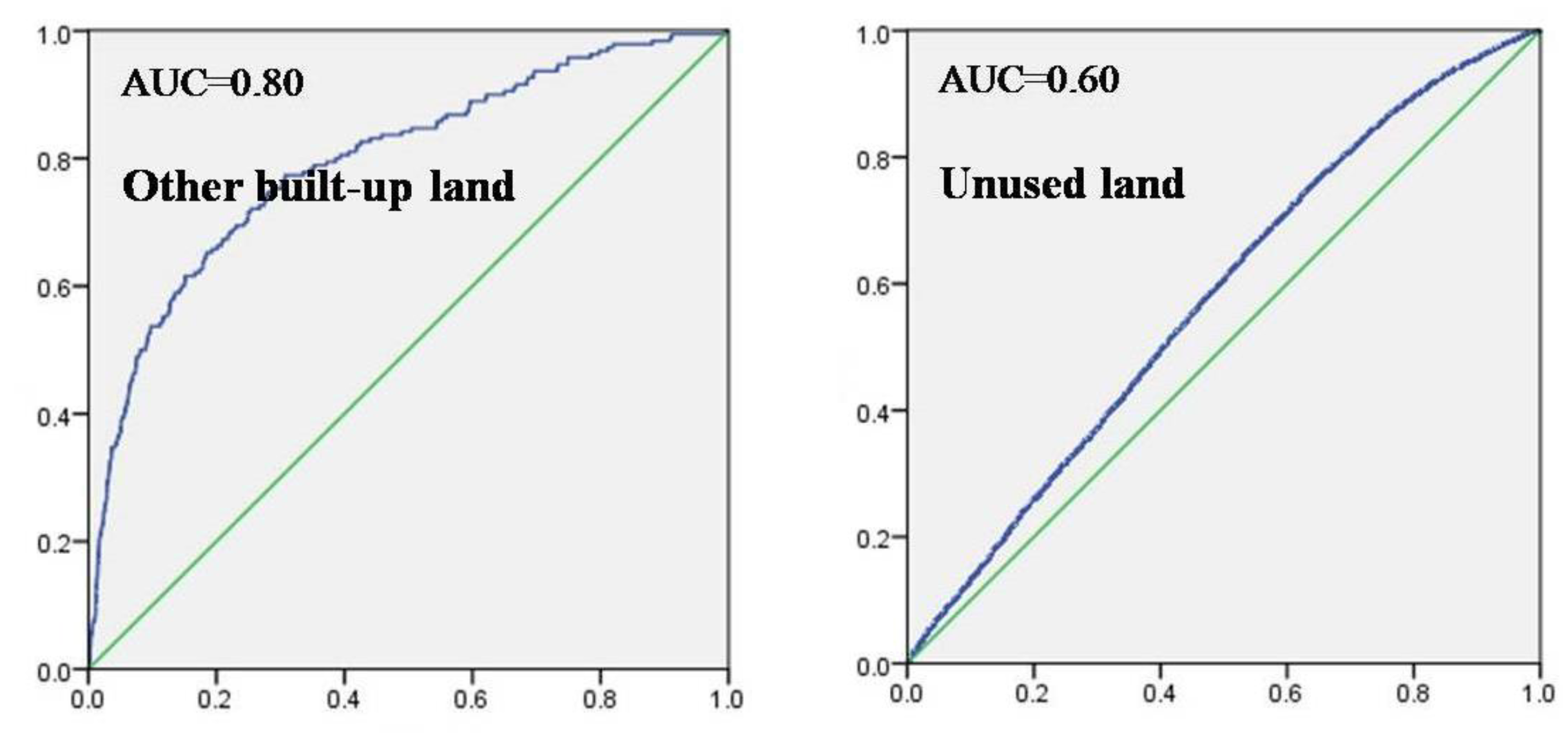
The training module is primarily responsible for two tasks: the first is to determine the structure of MLP and the second is to acquire the internal transformation rule through training data and target data and then output the probability of occurrence of different land use types. Meanwhile, a certain amount of training data and verification data are selected in the training process to verify the accuracy of the constructed MLP. Only the internal transformation rules produced from training under satisfactory training accuracy and verification accuracy are applicable to subsequent studies; otherwise, the data must be selected again, and the above training process must be repeated.
After the probability of occurrence of different land use types is determined, the external transformation rules are set in accordance with actual needs. The external rules include the quantity of land use types, the absolute restricted area, ecological sensitivity, neighborhood influence, land transfer cost, and the self-adaptive inertia coefficient.
(a) Quantity of land use types
Quantity of land use types reflects the development direction of land use. The sum of the areas of different land use types at different times is constant and is equal to the total land area. It can be expressed as a function:
where total area is the total land use area.
x1 to
xn are areas of different land use types. n is the land use type. The quantity constraint is used as the overall control during land use allocation. In other words, the quantity of land use transformation at a certain time, which is an essential constraint, is determined. Quantity of land use can be gained from the land use distribution map during a certain period; future quantity of land use is based on the simulation results.
(b) Absolute restricted area
The absolute restricted area is the area where land use transformation is restricted. The allocation of this region cannot be changed. These areas generally include cliffs, natural reserves, extensive water surfaces, and basic farmlands protecting regional food safety. The absolute restricted areas data are binary data with values of 0 or 1. A value of 1 reflects an absolute restricted space, indicating that land use transfer is prohibited in this region. A value of 0 indicates non-absolute restricted space, meaning that land use transfer is allowed in this region.
(c) Ecological sensitivity
To achieve maximum ecosystem service functions in national key ecological function zones, ecosystem structures and functions must be kept in the most stable state and must protect the maximum value of the ecosystem service. Hence, ecological sensitivity is added as another constraint in this study. Ecological sensitivity restricts transfer among different land use types to some extent. The factor weighting method is usually applied for ecological sensitivity evaluation. Ecological sensitivity can be expressed as:
where f(x
k) is the comprehensive value of ecological sensitivity. x
1 to x
n are influencing factors. In this study, slope, altitude, land use type, river, geological disaster liability, and soil erosion were chosen as the main influencing factors for the evaluation of ecological sensitivity. α1 to α
n are the weights of different influencing factors; they are determined by the analytic hierarchy process (AHP).
Based on the ecological sensitivity evaluation results, regions ranking in the top 20% (regions with high ecological sensitivity) are viewed as regions where land transfer is prohibited; these are set as 0. The remaining 80% of regions (regions with small ecological sensitivity) are viewed as regions allowing land transfer; these are set as 1.
(d) Neighborhood influence
Cellular expansion is influenced by cells in a neighborhood except for itself. In the MLP-CA model, the neighborhood analysis window was set as 7×7 to define the influence of neighborhood cells on central cells. The neighborhood function is defined as:
where
is the extent of grid cells affected by neighboring land use type j at time t, and
represents the total number of grid cells occupied by land use type j at the last iteration time
t–1 within the 7 × 7 window. wk is the variable weight among the different land use types, because there are different neighborhood effects for different land use types.
(e) Land transfer cost
Land transfer cost is mainly used to reflect difficulties in transformation among different land use types. When it is difficult to transform a particular land use type into another type, the land transfer cost is relatively high. When it is easy to transform a land use type into another type, the land transfer cost is relatively low. Land transfer cost is binary and is expressed as 0 or 1. Regions with low land transfer cost are 0, while regions with high land transfer cost are 1.
(f) Self-adaptive inertia coefficient
A self-adaptive inertia coefficient for each land use type is defined to auto-adjust the inheritance of the current land uses on each grid cell according to differences between the macro demand and the allocated land use amount. The inertia coefficient is defined as:
where,
denotes the inertia coefficient for land use type j at iteration time t.
and
denote the difference between the macro demand and the allocated amount of land use type j at iteration time t−1 and t–2, respectively.
Next, the possibility of occurrence of land use types, which is generated automatically in the training model, as well as neighborhood influence, land transfer cost, and the inertia coefficient are combined to construct a comprehensive transfer probability index:
where
is the comprehensive probability for cell i to transfer from the original type to type j at time t.
is the probability of occurrence of land use type j on cell i.
is the neighborhood expansion factor of land use type j on cell i at time t.
is the inertia coefficient of land use type j at time t.
is the transfer cost of the original land use type c to the target type j.
After obtaining the comprehensive transformation probability of the cells, the spatial allocation of land use is accomplished in the simulation module by superimposing a restriction area, ecological sensitivity constraints, and the quantitative structure of land use. However, there may be conflicts among the different rules in the allocation process. For example, a cell might be transferred from forest to farmland in view of the comprehensive transformation probability, but the cell might belong to a restricted area with land use transfer prohibited. Hence, several principles are defined in case of conflicts among transformation rules. (1) The preferential principle of the ecology: different land use types are distributed according to the following order: forest > grassland > waters > farmland > urban settlement > other built-up land > rural settlement > unused land; (2) The principle of maximum comprehensive transformation probability: taking forest, for example, different grids are ordered according to the comprehensive transformation probability [
22]. The grids with the highest transformation probability (forests) are recognized. The grids are ranked from high to low transformation probability until the desired total amount of forest is met.


