An Approach Based on Landsat Images for Shoreline Monitoring to Support Integrated Coastal Management—A Case Study, Ezbet Elborg, Nile Delta, Egypt

Abstract

Monitoring the dynamic behavior of shorelines is an essential factor for integrated coastal management (ICM). In this study, satellite-derived shorelines and corresponding eroded and accreted areas of coastal zones have been calculated and assessed for 15 km along the coasts of Ezbet Elborg, Nile Delta, Egypt. A developed approach is designed based on Landsat satellite images combined with GIS to estimate an accurate shoreline changes and study the effect of seawalls on it. Landsat images for the period from 1985 to 2018 are rectified and classified using Supported Vector Machines (SVMs) and then processed using ArcGIS to estimate the effectiveness of the seawall that was constructed in year 2000. Accuracy assessment results show that the SVMs improve images accuracy up to 92.62% and the detected shoreline by the proposed method is highly correlated (0.87) with RTK-GPS measurements. In addition, the shoreline change analysis presents that a dramatic erosion of 2.1 km² east of Ezbet Elborg seawall has occurred. Also, the total accretion areas are equal to 4.40 km² and 10.50 km² in between 1985-and-2000 and 2000-and-2018, respectively, along the southeast side of the study area.

1. Introduction

Coastal zones are extremely important for countries with highly populated coastal areas. Consequently, there is a concern about their future, particularly on the state of their natural resources, which provide life support and opportunities for economic development and tourism [1]. For this reason, models are developed to support Integrated Coastal Management (ICM) [2].

From this perspective, coastal management retains a crucial importance in order to shape economic and social objectives, especially for places with large sea resources. To accomplish such objectives, coastal monitoring surveys have been established to collect data useful for studying beach evolution and storms responses, identification of suitable sites for construction of harbors, shoreline protection plan, eco-system conservation, nourishments and dredging activities [3].

Ezbet Elborg is one of the most pivotal cities on the Egyptian coast, which is located at the northeast of Nile Delta, called Damietta branch. Fishing is the main socio-economic activity of this coastal region with about 60% of all Egyptian fishing activities existing in Ezbet Elborg while the agriculture and animal husbandry contribute to a certain extent [4]. Before Constructing Aswan High Dam (AHD), the sediments discharge from Damietta branch to the Mediterranean Sea was estimated to be about 0.6 to 1.8 million m³/year [5], which caused shoreline progression to the sea. After building AHD, the coast began to dramatically erode as the flow and sediments discharged to the sea became very negligible. Accordingly, Damietta beach has been suffering, since 1970, from a severe erosion [6]. Therefore, in the year 2000, the Egyptian government, represented by the Shore Protection Authority (SPA), constructed a 6 km seawall to protect this area from erosion. Also, according to the development plan of Damietta Governorate, a new fishing port is proposed in this area to provide life support and opportunities for economic development. For this reason, this study will be helpful for supporting management and monitoring of coastal area changes at Ezbet Elborg region.

Shoreline monitoring has widely supported ICM plans and policies. For instance, Dibajnia et al. [7] presented a national shoreline management plan (SMP) to the Ports and Maritime Organization of Iran that is useful for addressing existing coastal problems and setting policies that show shoreline management as part of ICM policy dealing with existing and planned development in coastal areas. Goncalves and Wange [1] evaluated three of the most commonly used GPS-based shoreline monitoring methods: relative kinematic (RK), real-time kinematic (RTK) and precise point positioning (PPP) methods. Their results highlighted the issues and important considerations in choosing an economically viable GPS method for mapping shoreline changes, particularly for supporting ICM policies. Valentini et al. [3] presented a monitoring system deployed in 2015 in the Apulia region (South Italy), aimed at supporting management and monitoring activities of coastal areas. Video stations are installed at two different sites, characterized by different geographic exposition and wave climate. The shoreline extraction and the data post processing are based on new algorithms automatically working on Timex images, providing a calculation of shoreline evolution and cross-shore profiles. The video system employed improves the actual available methodologies for shoreline extraction. Samaras and Koutitas [8] presented a new shoreline evolution model for quantifying the impact of watershed management on coastal morphology, using an integrated methodological approach. The approach is based on the consideration of the watershed and the coast as a spatiotemporal continuum in the ICM framework by utilizing the capabilities of numerical modeling to simulate the evolution of the phenomena in both fields and thus quantifying their correlation. On the other hand, for improving the ICM concepts, better understanding and knowledge of coastal dynamics and shoreline erosion due to hard structures such as seawalls are required. Many studies have investigated the effect of seawalls construction on adjacent beaches and coastal dynamics. Ismail and El-Sayed [9] examined numerically the sea-bottom morphology and cross shore profiles in front of Rosetta seawalls which constructed in 1990, on the Nile Delta coastline to decelerate coastal erosion of the headland after the operation of the (AHD) in 1965. The results showed that a significant component of sediment scour, in front of the seawall, is manifested as an offshore sediment transport current. Thereafter this offshore current is deflected alongshore contributing to sediment accretion down drift the seawall. Balaji et al. [10] studied the effects of seawall along the coast of Fansa, India, using a combination of numerical modelling, theoretical modelling and geo-informatics. They found that the construction of the seawall resulted in a landward erosion of about 20 m in the down-drift direction of the seawall, within a year of construction. Also, the beach is further predicted to erode by another 20 m before attaining the state of equilibrium by the year 2014. This estimation is successfully validated through remote sensing-based analysis, the results of which confirm that the landward erosion from 2011 to 2014 is approximately 40 m in the northern side of the sea wall.

Long-term monitoring of shorelines changes by comprehensive field surveys is costly, labor-intensive and time-consuming. Therefore, as per the availability of satellite images at different dates for same locations, remote sensing is one of the best solutions for monitoring coastal changes over a long period as it is a cost-effective method [11,12,13,14].

Satellite images features extraction has been studied by several researchers. For instance, the Normalized Difference Water Index (NDWI) along with the Red, Green and Blue (RGB) system provide an excellent delimitation of the coastline [15]. Di, et al. [16] presented a semi-automatic method to extract a shoreline from a commercial Earth observation satellite (IKONOS) image., The method is based on mean shift segmentation, major water body identification, initial shoreline extraction and shoreline refinement. Dewidar and Frihy [17] used digital shoreline analysis software (DSAS) to calculate the annual rate of beach changes for detecting pre and post-beach response to protection structures constructed north-west the Nile delta. They found that historical Landsat data can be applied for change detection analysis of rapidly changes highly energetic coastlines. El Banna and Herher [18] detected temporal coastline changes by analyzing satellite Landsat images for the Mediterranean coast of northern Sinai for the years 1986 and 2001 for monitoring shorelines changes and their associated sediment characteristics. Giannini and Parente [19] used Quickbird multispectral images to extract coastline where, segmentation is performed using all multispectral bands of the satellite dataset. Then, classification is performed using both segmented images as well as NDVI (Normalized Difference Vegetation Index) map to discriminate accurately between the water and no water for extraction of coastlines. Numerous studies for extracting shoreline via remote satellite images have been discussed by References [20,21,22,23,24,25]. Also, mapping shorelines was carried out using supervised approaches such as the machine learning techniques. Zhang et al. [26] presented Support Vector Machine (SVM) classification algorithm to coastline extraction, they checked different SVM kernel functions such as Polynomial, Radial basis and Sigmoid and they found that the Sigmoid kernel function outperforms other functions. Yun and Myung [27] compared the water-index-based method and SVM algorithm for plotting accurate shorelines using high-resolution satellite images. The results showed that both techniques accurately identified coastal zones with the SVM outperformed the water–index for coastal zones with irregular shapes and shaded areas.

The resolution of the satellite images is the main constraint for mapping which governs the accuracy and precision. However, coastal areas are spatially and optically more complex and require more frequent spatial and spectral sampling to enhance the monitoring ability and assessing the dynamics of the coastal processes [28,29,30,31,32,33]. Despite this, few of these studies checked the accuracy of the derived shorelines via image classification technique, especially in Egypt.

The aim of this study is to investigate the shoreline changes in the northeast of Nile Delta, Egypt, which is exposed to obvious changes in the coastline, due to a combination of natural and anthropogenic factors. Construction of dams across the Nile River, such as AHD, reduce the sediment flux into the sea. Consequently, coastal erosion is produced in the delta. This erosion has been diminished due to hard structures such as jetties, detached breakwaters and seawalls at eroded promontories. This study is implemented in the area of Ezbet Elborg, northeast of Nile Delta, Egypt, for supporting management and monitoring of coastal area changes. This location was selected because there are numerous socio-economic activities that are taking place; so, the present study would be helpful for the design of the proposed fish port in this location. To achieve these objectives, a novel method is developed to assess the shoreline change based on the combination of SVMs classification for Landsat images and GIS to improve the accuracy of shoreline estimation. Accordingly, changes of the shorelines every five years during the period between 1985 to 2018 including seawall effects are evaluated. The present study is organized as follows. The Introduction starts with the state-of-the-art of the problem. Then, the study area information and the corresponding coastal processes are presented. The next section describes the details of the collected Landsat images, a brief description of SVMs technique is introduced, the methods of accuracy assessment for classified images is presented. Also, the proposed method for the Shoreline changes detection. Then, the obtained results are presented and compared with field data.

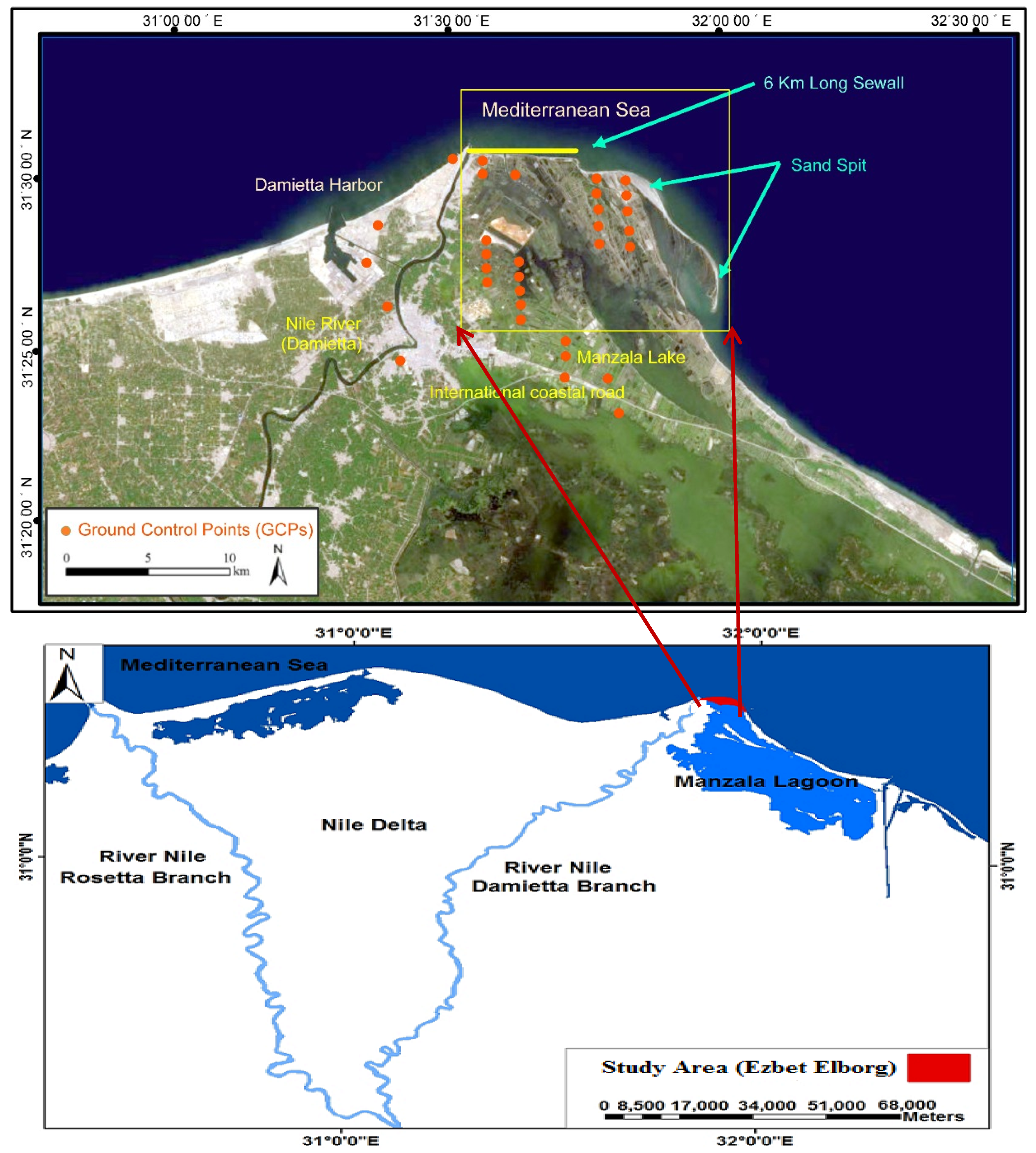
2. Study Area

The study was carried out along the shoreline of Ezbet Elborg city located next to the tip of Damietta promontory on the north-eastern Nile delta coast. The coastline of the study area extends about 15 km east of Damietta with 6 km long seawall that constructed in year 2000 along the eastern side of the Nile’s mouth for protecting the shore from erosion as shown in Figure 1. The study area lies between latitudes 31°26′00″ N to 31°32′00″ N and longitudes 31°54′00″ E to 32°20′00″ E. The beach of the area consists of loose quartz sand merged with little amounts of heavy minerals and shell fragments. Moreover, the southeast of the study area is distinguished by developing sand spits due to longshore sediment transported directed to the east by the prevailing northwest waves along the Nile Delta coast; in addition, the quasi-concave shoreline shape helps the evolution of sand spit [34]. Directional wave measurements for the study area in 2010 showed that recorded maximum wave height during the storms is almost 6.0 m, while significant wave height is 4.2 m from N. The monthly maximum peak wave period varies between 7.0 and 13.2 s. The direction of a predominant wave throughout is from the N-NW (86%) sector for all months (mainly from NNW (49%) direction). The littoral current movement is generally towards the east with an average velocity about 34 cm/s. Damietta promontory coast is of micro-tidal semi-diurnal nature with a range of the order 25–30 cm [35].

3. Materials and Methods

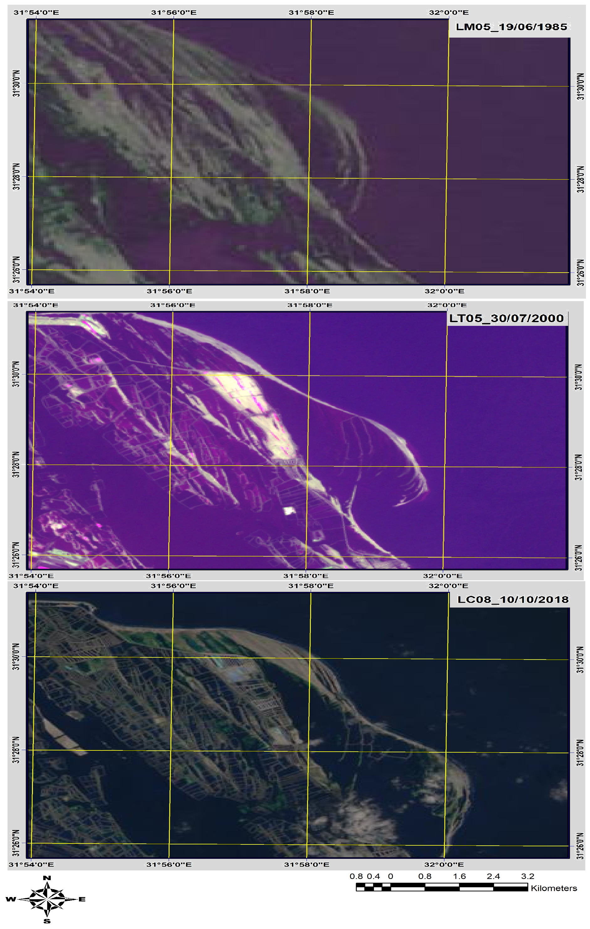
3.1. Satellite Images and Pre-Processing

A series of Landsat images were used in this study every five years between 1985 and 2018, as presented in

Table 1. Details of the satellite dataset used in this study.

Satellite and Sensors	Path/Row	Date of Acquisition	Spatial Resolution	Acquired Time (hh:mm:ss)	Tidal Level (cm)
Landsat 5 (TM)	177/38	19-06-1985	30 m	07:51:28	…….
Landsat 5 (TM)	177/38	16-05-1990	30 m	07:37:12	…….
Landsat 5 (TM)	177/38	09-02-1995	30 m	07:53:14	…….
Landsat 5 (TM)	177/38	30-07-2000	30 m	08:00:38	30.7
Landsat 7 (ETM)	177/38	28-07-2005	30 m	08:07:22	38
Landsat 7 (ETM)	177/38	14-10-2010	30 m	08:13:25	42
Landsat 8 (Oli/TiR)	177/38	24-07-2015	15 m	08:07:18	36
Landsat 8 (Oli/TiR)	177/38	10-10-2018	15 m	08:10:04	32

. Eight Landsat images were taken into consideration spanning the time period between 1985–2018. Those images were downloaded from the U.S. Geological Survey (USGS) Earth Explorer Web Tool (https://earthexplorer.usgs.gov/). Most of Landsat images are in good quality with lowest cloud coverage. Also, the time-series satellite dataset must be collected at similar tidal levels to compare the shorelines at different times as shown in Table 1 [36,37].

Geometric distortions are normally introduced to satellite data during acquisition. They result from several factors including attitude (roll, pitch and yaw) or in other words, the Earth’s rotation and panoramic distortions. Remotely sensed scene coordinates do not, therefore, coincide with a standard map projection and the coordinates of fixed point vary from image to image. Hence, geometric correction (rectification) is needed for removing geometric anomalies and create a faithful representation of the original scene by correcting pixel location errors and establishing a coincidence between ground attributes and the incorrect position throughout the image [38]. The geometric correction of each Landsat image is carried out using standard procedures [38]. First, the data from image coordinates (i.e., lines and pixels) is transformed to geographic coordinates (i.e., latitude and longitude or UTM, etc.) by selecting pairs of GCPs—one from the image and the other from a map—for the same location. This is repeated for several locations across the whole scene till the best transformation fit is established. This process, named rectification, corrects the distortion in the input image. Then, the rectified image is resampled as the position of the pixels in the geometrically corrected image differ from those in the original image, the software follows a pre-defined sampling strategy to determine which source pixels should be used to define each georeferenced pixel [38].

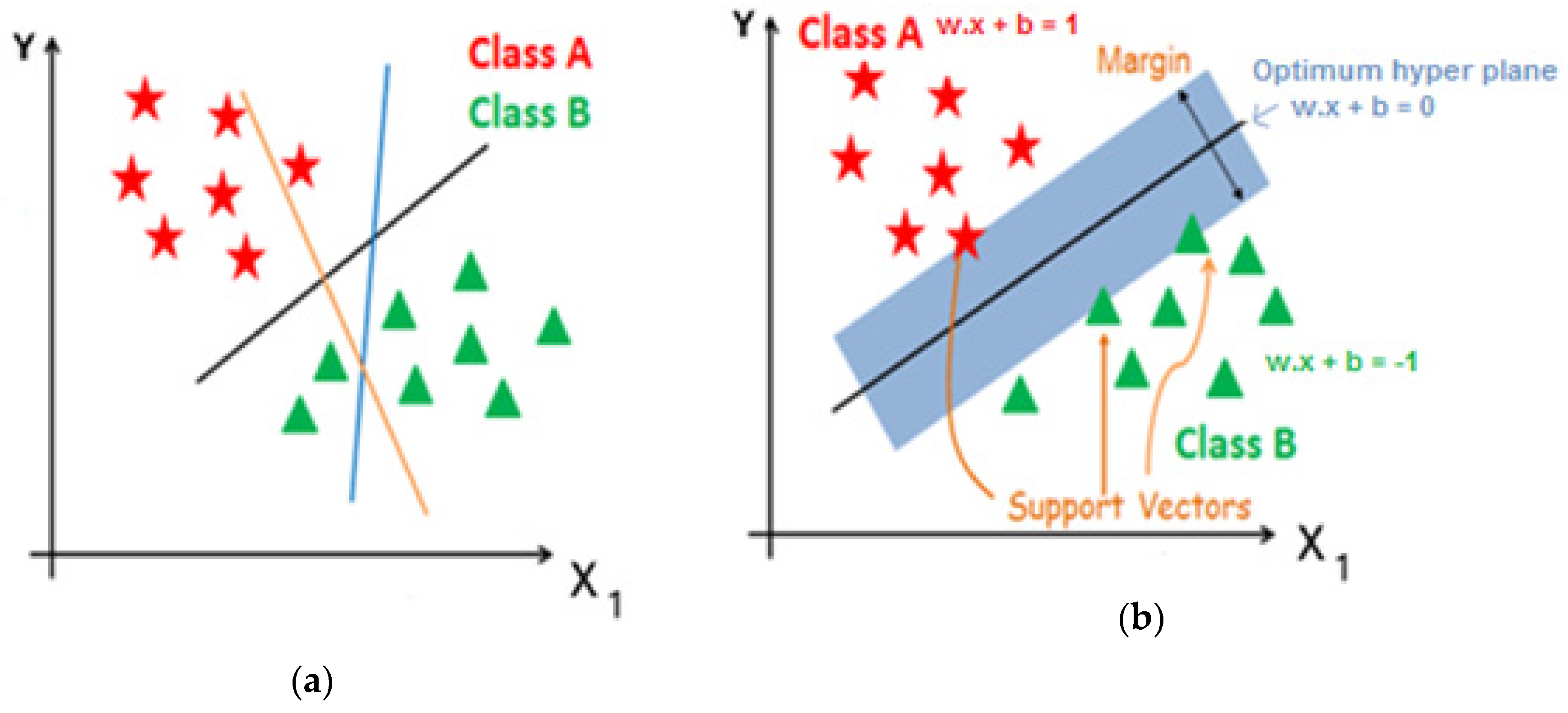
3.2. Images Classification

Shoreline image classification was made for improving the accuracy of extracted shoreline change. Image classification techniques relies on many factors, such as the complication of the landscape in the study area, chosen remotely sensed data, choice of suitable classification methods and assessment of classification accuracy [39].

In this paper, SVMs were used to extract coastline from remotely sensing images. The SVM classification algorithm is considered the best method for problems of small sample, nonlinear and high dimension [40]. SVM has higher performance in terms of training speed and classification accuracy than other techniques when used for classifying remote sensing images; it does not need to reduce data dimensionality. It solves the common difficulties of artificial neural networks and other methods, such as difficulties associated with identifying network structure, over-learning and local minima [26].

Basically, the main idea of SVM is the selection of an optimal hyper plane, which can be used for linear classification of separable patterns. The optimal hyper plane can be defined as the plane that maximizes the distance from the hyper plane to the nearest point of each pattern which called a margin. As shown in Figure 2a, there exist many hyper planes but only one can provide the maximum margin between the two classes (Figure 2b) called the optimum hyper plane. Support vectors are the points located on the boundary of margin that define the hyperplane of maximum margin.

SVM is developed from the optimal classification surface in case of linear separable, for datasets {x_i, y_i} (i = 1, . . ., k) where x ϵ R^N in an N-dimensional space and y ϵ {−1, +1}. Its basic idea is to find the optimal classification surface (hyperplane) between the two types of datasets. As shown from Figure 2b, this hyperplane is defined as

$$\mathrm{w}*x_i+\mathrm{b}=0,$$

(1)

where, (w) is the weight vector of the classification surface, (x) is a point lying on the hyperplane and (b) is the bias of the distance of the hyper plane from the origin. For the linearly separable case, a separating hyperplane can be defined for two classes as:

$$\mathrm{w}*x_i+\mathrm{b}\ge 1.\mathrm{for} \mathrm{all} \mathrm{y}=+1$$

(2)

$$\mathrm{w}*x_i+\mathrm{b}\le 1.\mathrm{for} \mathrm{all} \mathrm{y}=-1.$$

(3)

These inequalities can be combined into a single inequality:

$$y_i(w*x_i+b)-1\ge 0.$$

(4)

If the optimal classification surface meets the condition in Equation (4), the phenomenon of linearly separable classes is executed [41]. Also, the SVM model uses a kernel function to separate classes which cannot be separated using line or plane. Therefore, a non-linear region is required by the classifier to separate such classes. This is also known as kernel trick, transformation of the data into higher dimensional feature space in order to separate it linearly.

By using the Lagrange multipliers, the dual formulation expressed in terms of variables ${\propto }_i$ is determined (also known as the dual representation of the decision boundary), an optimal desired weights vector of the regression hyper-plane is represented as:

$$w^{*}={\sum }_{i-1}^n\left( {\propto }_i-{\propto }_j\right) K\left( X_i-X_j\right).$$

(5)

Finally, SVM algorithm can be expressed as:

$$f\left(x\right)={\sum }_{i-1}^n\left( {\propto }_i-{\propto }_j\right) K\left( X_i-X_j\right)+b,$$

(6)

where $K \left( X_i-X_j\right)$ is the Kernel function which equals the inner product of two vectors $X_i$ and $X_j$ in the feature space $\varphi \left(X_i\right)$ and $\varphi \left(X_j\right)$ that used to compute a non-linearly separable function and then transform it into a higher dimension linearly separable function.

Kernel functions are used to change the dimensionality of the input space, in order to perform the classification task with more confidence. Zhang et al. [26] recommended the Sigmoid kernel function for optimal classification (Equation (7)), so it is used in the current study.

$$K\left( X_i.X_j\right)=\tanh \left[C\left(X_i.X_j\right)+b\right],$$

(7)

where, C and b are kernel function parameters.

3.3. Accuracy Assessment of Classified Images

Accuracy assessment or validation is a significant step in the processing of remote sensing data. Accuracy assessment parameters are useful for assessing the model performance regarding a particular category/class of specific interest for the study. The confusion matrix is the most widely used measure of image classification accuracy. It is simple cross-tabulation of the mapped class label against the observed or reference data in the ground for a sample set [42]. Several measures of classification accuracy can be obtained from a confusion matrix, in this study, both Overall Accuracy (OA) and KAPPA (Equation (9)) are used for accuracy assessment. The OA is obtained by dividing the total number of correctly classified pixels (n) by the total number of pixels (N), as follows:

$$OA=\frac{n\left( Total number of corrected pixel\right)}{N\left(Total number of pixel of raw image\right)}.$$

(8)

KAPPA analysis is a discrete multivariate technique used for assessing the accuracy of image classification [42,43]. It is generally a measure of agreement between the classified map and the reference data. According to Reference [43], the KAPPA statistic is computed as follows:

$$KAPPA\left(K\right)=\frac{N{\sum }_{i=1}^r{X}_{ii -}{\sum }_{i=1}^r\left(X_{i+}*X_{+i }\right)}{N^2-{\sum }_{i=1}^r\left(X_{i+}* X_{+i}\right)},$$

(9)

where; r = number of rows and columns in error matrix, N = total number of observations (pixels), Xii = observation in row i and column i, Xi+ = marginal total of row i and X+i = marginal total of column i.

Many schemes describing the strength of agreement of classification are based on the KAPPA coefficient. The categorization of KAPPA is reproduced by Rwanga and Ndambuki [42] as shown in

Table 2. Rating criteria of KAPPA.

Category No	KAPPA Statistics	Strength of Agreement
1	<0.00	Poor
2	0.00–0.20	Slight
3	0.21–0.40	Fair
4	0.41–0.60	Moderate
5	0.61–0.80	Substantial
6	0.81–1.00	Almost perfect

.

3.4. Comparative Study

To evaluate the extracted shoreline accuracy, differential-real time kinematic (DRTK) global positioning system (GPS) observations for shoreline were collected. The DRTK-GPS was used to estimate an accurate shoreline change [1]. The D-RTK GPS data was collected at the same period where the Landsat image was acquired in 2015 by walking along the shoreline of the study area, carrying portable DGPS Hemisphere R131 joined with marine laptop model Tetra Note-EX that continuously record the coordinates of the shore using hydrographic survey software (c-navigator). GPS data sets are projected in UTM projection with zone 36 north and WGS 84 datum.

3.5. Shoreline Indicators

Shoreline is defined as the line of contact between land and a body of water. It is easy to define but difficult to capture, since the water level is always changing [44]. Mapping shoreline changes as an input data is important for coastal hazard assessment such as tidal flooding, sea level rise, land subsidence and erosion-sedimentation. Multi-year shoreline mapping is a valuable task for coastal monitoring and assessment [44]. Due to the dynamic behavior of the idealized shoreline boundary and practical considerations, Boak and Turner [45] classified two groups of shoreline indicators from 45 examples. Classifications in the first group are based on a visually discernible coastal feature. The other ones are datum-based shoreline indicators that are determined by the intersection of the coastal profile with a specified vertical elevation defined by tidal constituents of a particular area, such as mean high level (MHL) or mean sea level (MSL). The amount of tidal correction can be large or small depending on the tidal range, the maximum correction amount can be a few meters in cases of large tidal range [20,46]. As the tidal change in the study area is very small, its impact on the shoreline change due to tide variation is very small. Therefore, this paper investigates the shoreline change and beach evolution of Ezbet Elborg using Landsat satellite images. The shoreline position extracted from a satellite image is a waterline or a wet/dry line that describes the instantaneous land-water boundary at the time of imaging similar to the first kind of shoreline indicator as used before in many studies [20,47]. Moreover, for minimizing the error, the Landsat images with similar tidal phases are considered in the present study as shown in Table 1.

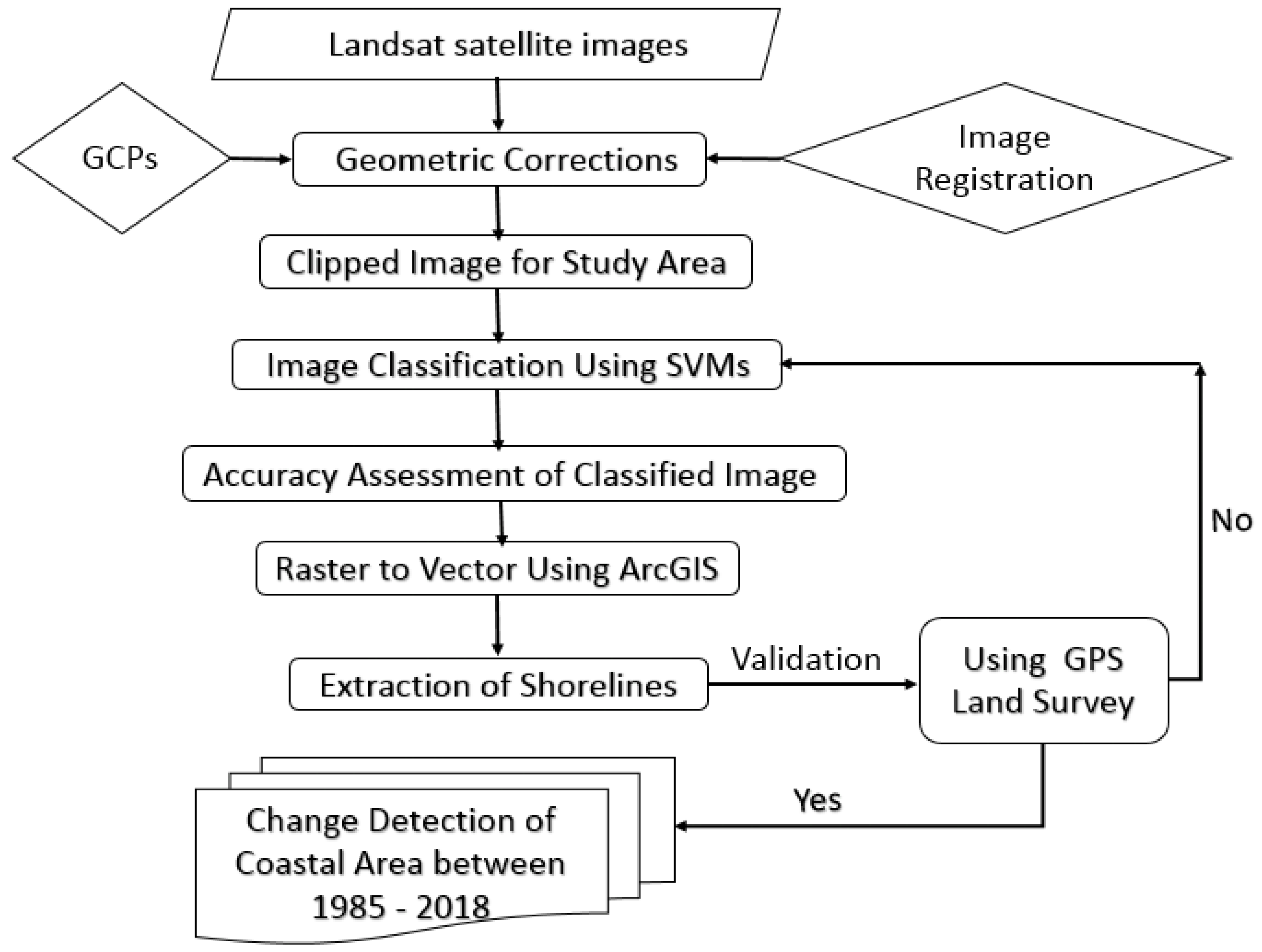
3.6. Proposed Method for the Shoreline Changes Detection

In this research, a post-classification comparison is applied for Ezbet Elborg shoreline changes detection, classified images are converted to vector layers by using Raster to Vector module using GIS software (ArcGIS 10.4.1). All shorelines extracted from classified images were overlaid and operated in a geodetic base in ArcGIS 10.4.1 software for detection change of shoreline. The process used in this study is presented in Figure 3 and described as follows:

• Image to Image registration process is implemented for all satellite images. The Satellite map from Google earth software was used as a base map to georeferenced the Landsat image acquired in 1985 through image to map referencing. Then, the Landsat image was considered as the master image that was utilized to register other images through image-to-image registration. To accurately register each image, a total of at least 35 ground control points (GCP) was examined and matched with all images. These points include: road intersections, prominent geomorphologic features and river channels as shown in Figure 1. After rectification, the root mean square error (RMSE) for the deviations between the GCP and GP location is determined and kept smaller than 0.45 pixels to ensure a good geo-referencing of the images. The images of the study area are extracted by clipping it from the registered satellite images based on GIS solution.
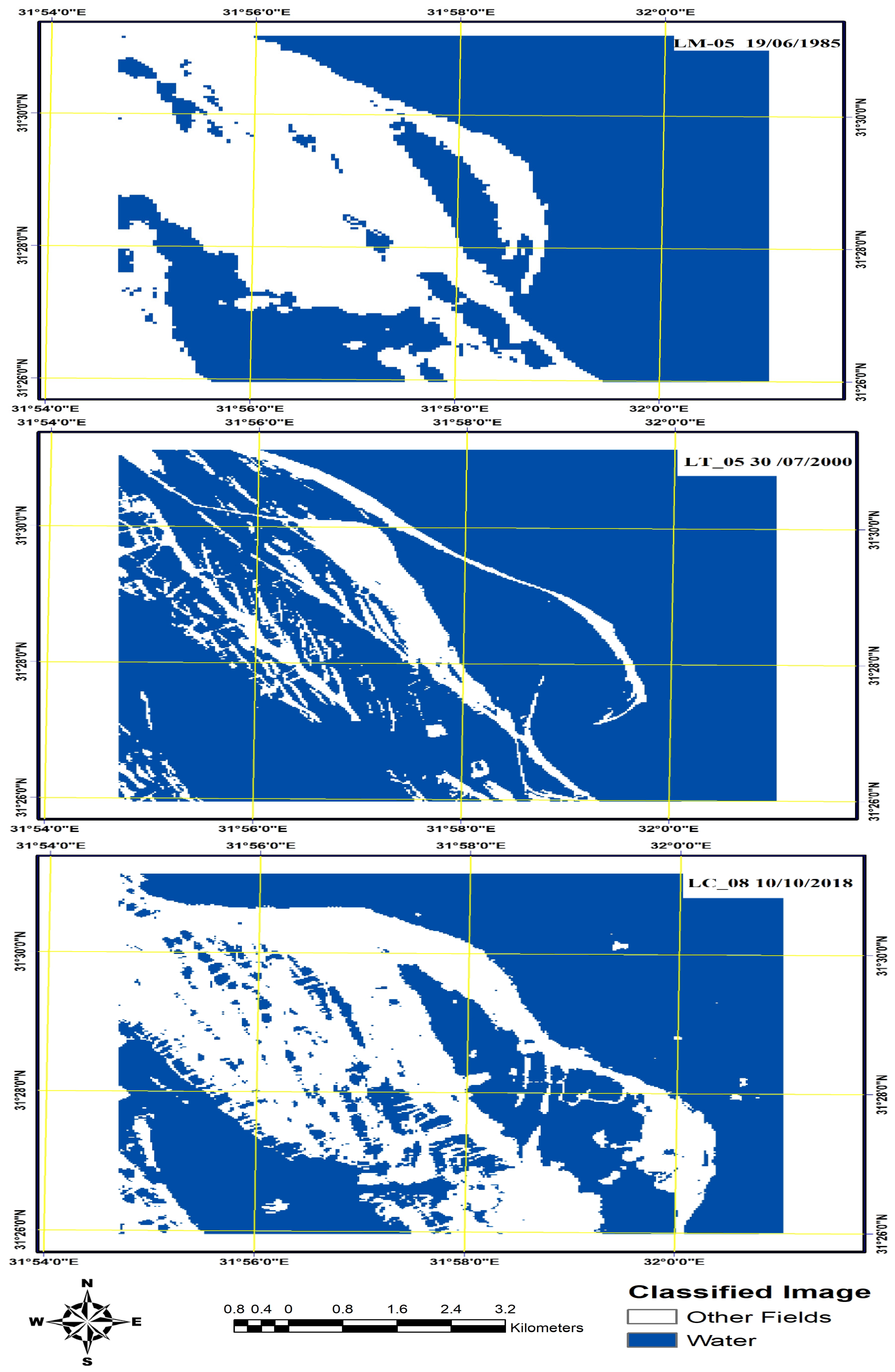
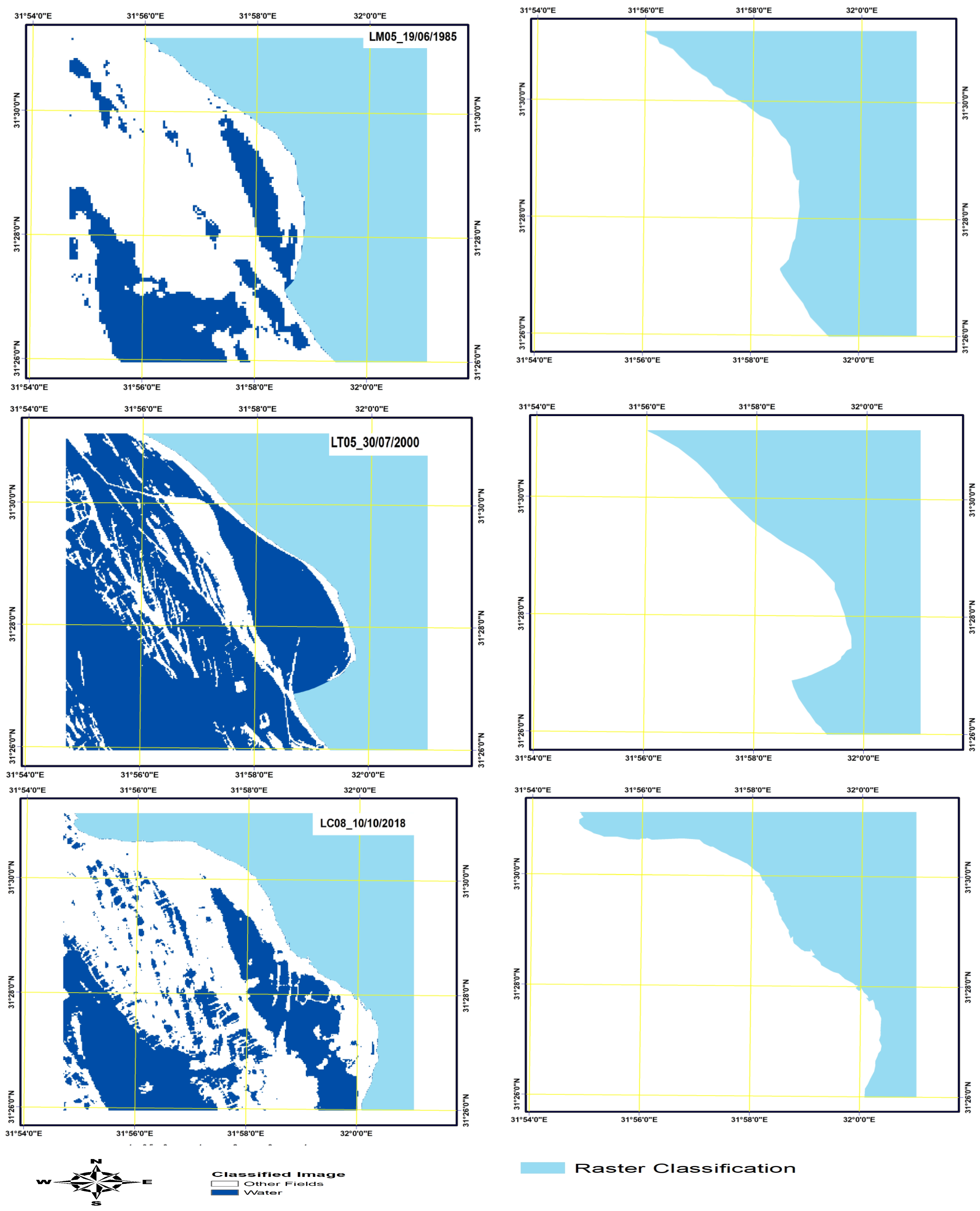
• Image classification is done using SVMs. The SVM algorithm is designed using MATLAB software. By this classification, two classes are created and called “Water” and “Other-Fields.”
• Image classification accuracy is determined as presented before in the “image classification” section. KAPPA coefficients are then calculated and evaluated.
• The classified image is converted to vector layers using ArcGIS to extract shorelines.
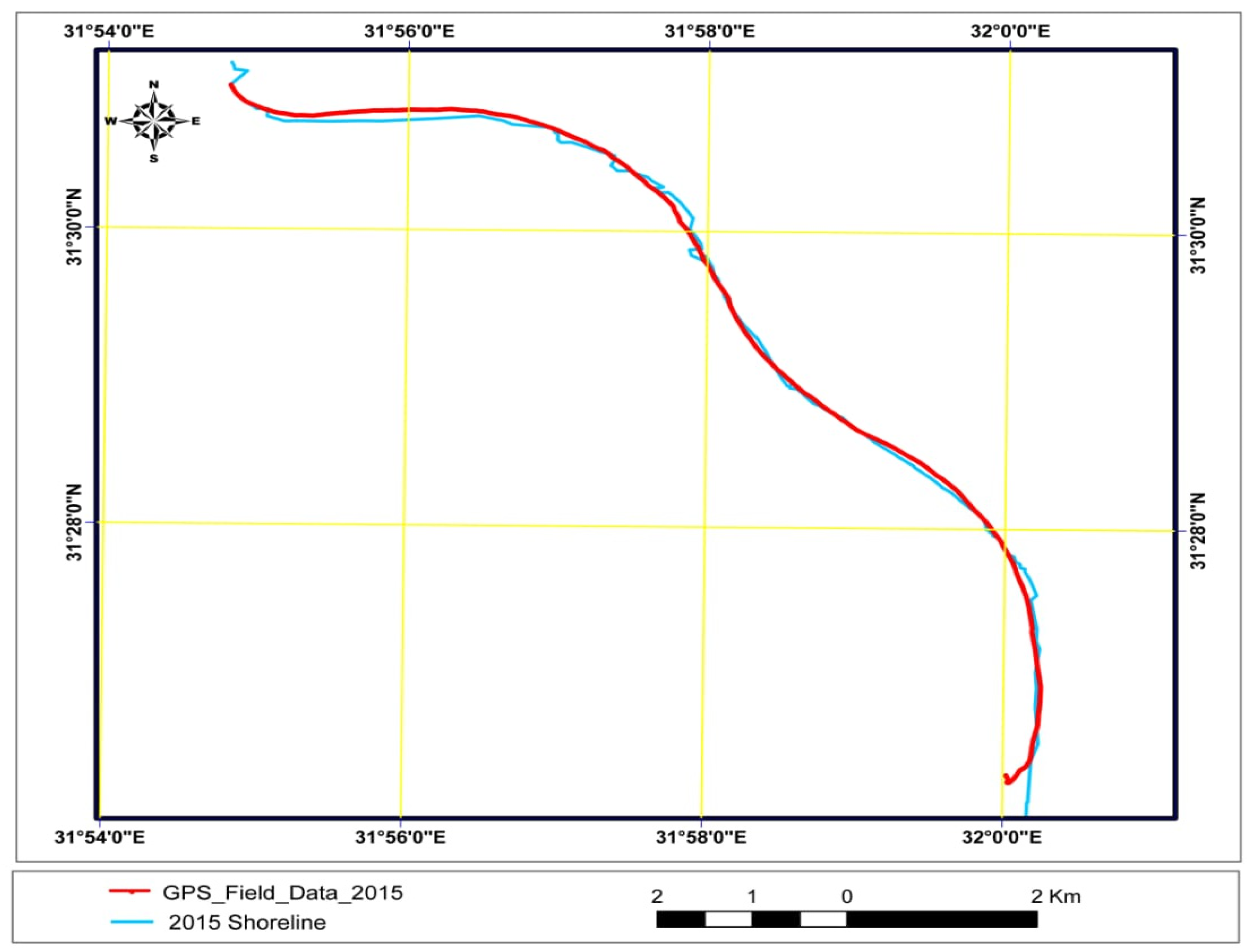
• Additional verification is done by comparing the extracted shorelines using the proposed approach with the GPS land survey to evaluate its applicability to monitor shoreline changes.
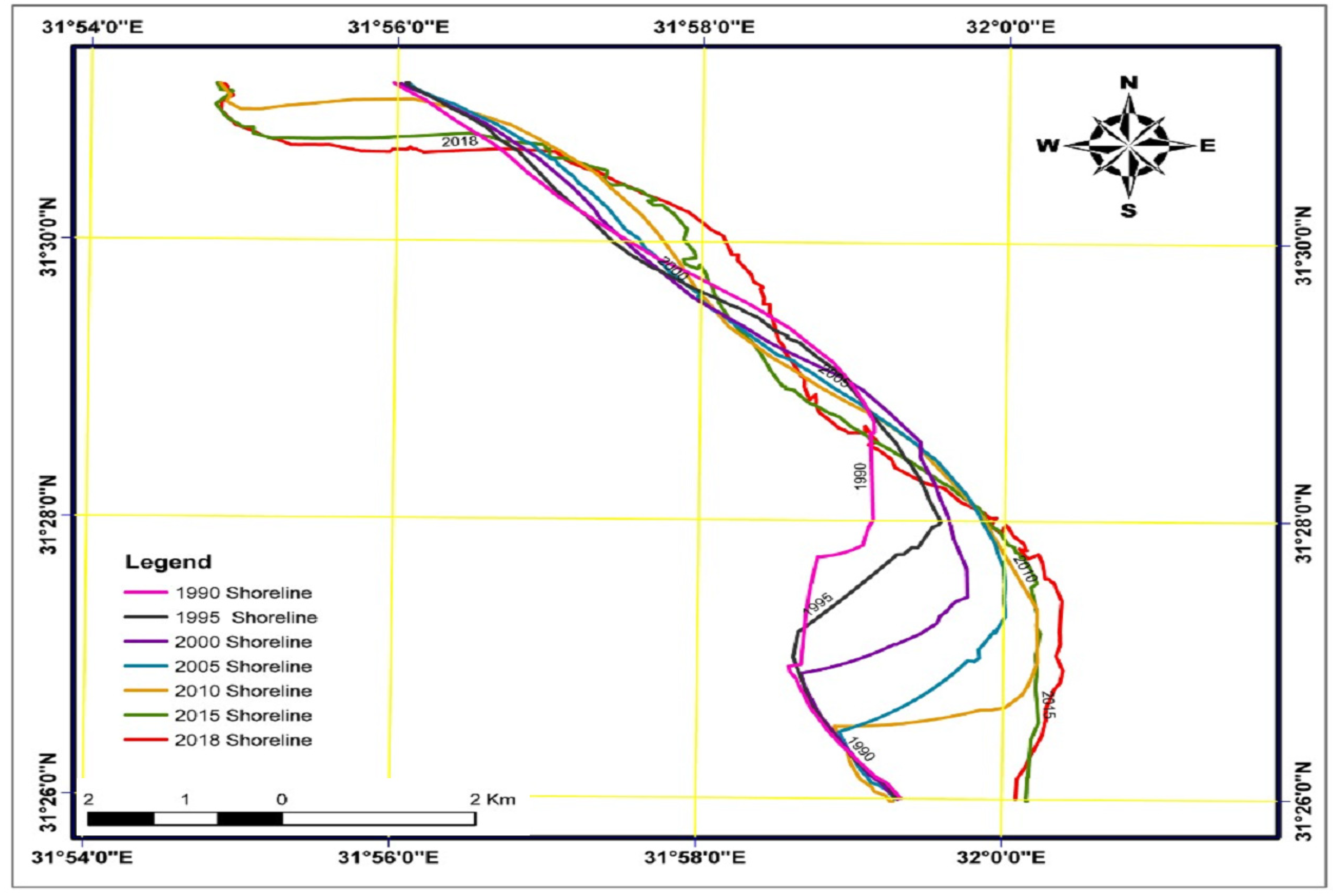
• Finally, change detection of coastal areas is studied using the generated vector maps by the ArcGIS.

4. Results and Discussion

Figure 4 illustrates the original satellite image of the study area which clipped from registered images of years 1985, 2000 and 2018. The actual shoreline position is determined using the SVM classifier with sigmoid Kernel function to categorize the trained samples into two classes named “Water” and “Other-Fields” from Landsat images, as shown in Figure 5. Also, the classification accuracies of the classified images are calculated (

Table 3. Overall Accuracy (OA) and KAPPA statistics of the images.

Date of Satellite Image	OA	KAPPA Statistics
19-06-1985	86.0%	0.74
16-05-1990	89.0%	0.76
09-02-1995	90.0%	0.77
30-07-2000	92.0%	0.79
28-07-2005	94.0%	0.79
14-10-2010	95.0%	0.84
24-07-2015	97.0%	0.86
10-10-2018	98.0%	0.86

). From Table 3, the final accuracy assessment revealed that the average OA of the classification accuracy is 92.625% and the average KAPPA agreement coefficient is 0.8. Accordingly, the classification is rated as substantial based on the KAPPA agreement coefficient and hence the classified images can be used for detecting shoreline changes. Then, each classified image is converted to vector layers using Raster to Vector module to convert the pixels representing the seaside into vector layer to get the actual position of shoreline as shown in Figure 6. It is noted that the blue areas noticed in the left part of the picture (Figure 6) are fish farms.

To extract the shoreline, the distance between the shoreline positions produced from the current analysis and fixed polygon is measured to provide a reliable record for monitoring the changes of the shoreline positions over the 33-year time frame. For validation, the extracted shoreline from the Landsat images is compared with the shoreline identified by the ground survey performed by the Coastal Research Institute (CORI) in 2015 as shown in Figure 7. It is found that the correlation coefficient between the Landsat images and field data is 0.87, which reflects the validity of Landsat images to detect shoreline changes.

All shorelines extracted from the classified images (Figure 6) are overlaid and operated in a geodatabase using the GIS software as seen in Figure 8. From Figure 8, it is seen that the shoreline behavior is dramatically changed during the monitoring time. The shoreline length is increased by 7.52% and 31.31% during the years 2000 and 2018, respectively, relative to the shoreline length in 1985.

Figure 9 and

Table 4. Coastal areas change of the study area.

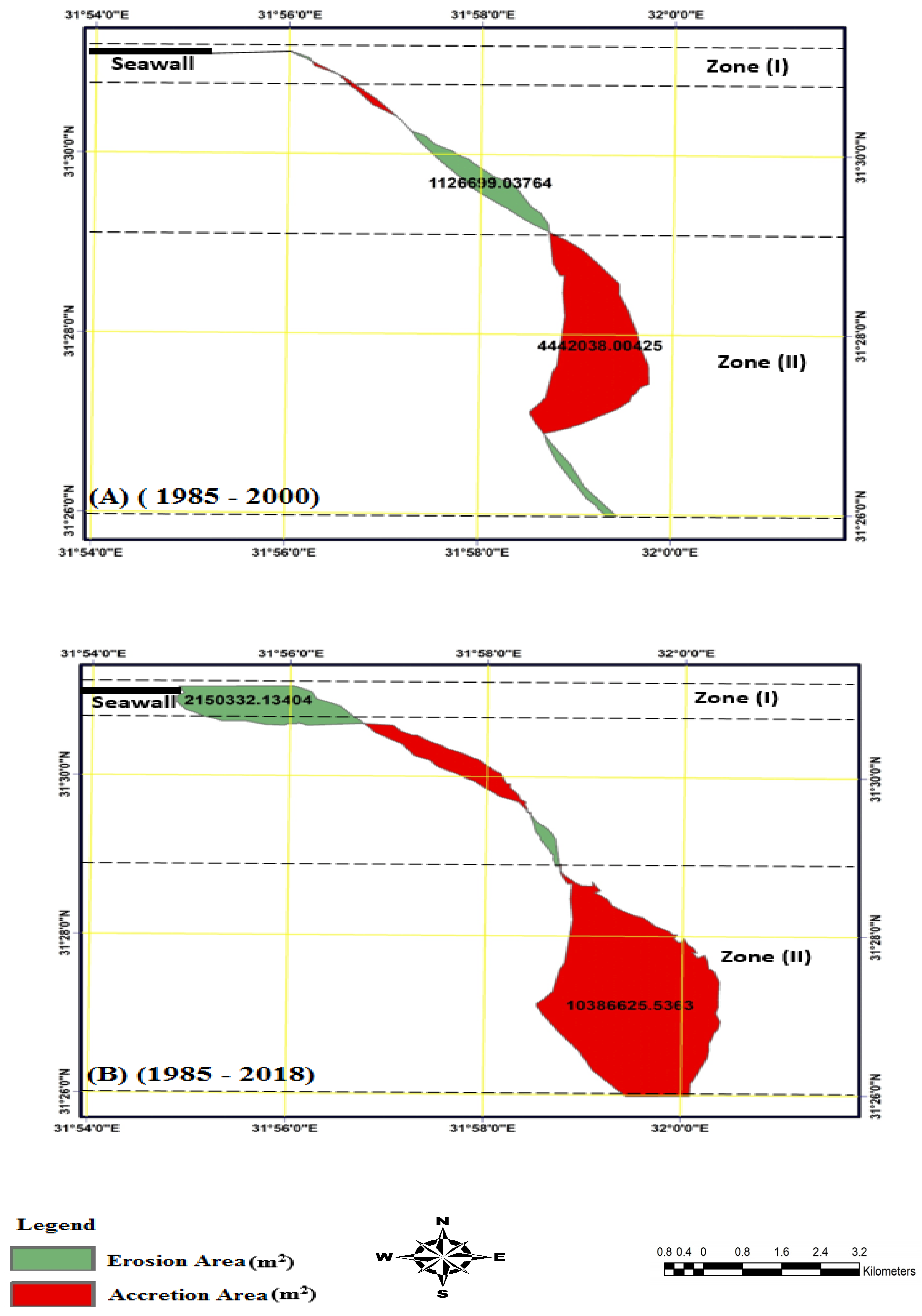
Date	Area (m2)		Rate of Change (m2/year)
	Erosion	Accretion	Erosion	Accretion
(1985–2000)	1,126,699	4,442,038	75,113	296,135
(1985–2018)	2,150,332	10,386,625	65,161	314,746

demonstrate the changes of the coastal area for the years 2000 and 2018 according to the base map. Along the area of erosion/accretion, an overview of the historical coastal dynamic can assist in better explanation of other features of the morphological phenomena occurred. Erosion at the eastern side of Damietta Promontory had begun after the construction of the AHD and continued until the construction of the 6 km seawall at year 2000 as shown in Figure 1. The erosion rate was 53 m/year during the period 1990 to 1999 [48]. The seawall successfully stopped the erosion at proposed area and the shoreline is relatively stable (Figure 9A; Zone I) but the erosion was shifted to the leeside of the seawall with high rates 59 m/year as seen clearly in Figure 9B; Zone I and

Table 5. Comparison between previous studies and the present study.

Research	Time Period	Average Annual Retreat (m/year)	The Used Technique
Esmail et al. [48]	1990–1999	54	Iso cluster technique, Threshold method, On screen digitizing method.
	1999–2003	61.5
	2003–2015	54.5
El-Asmar et al. [50]	2003–2011	61.45	On screen digitizing method
Present Study	2000–2018	59	Digitizing as line feature based on SVM Classifier.

. Also, the maximum shoreline progress (1950 m) during the period (2000–2018) was recorded for the southeast of the study area with maximum accretion 124 m/year that causes the increase of spit area from 4.4 km² to 10.38 km², approximately (6 km²) net area, pre and post the construction of the seawall (Zone II) due to the movement of littoral drift of sand at the seawall lee after its construction with the seasonal NE wave action. El-Banna and Frihy [49] indicated that Damietta spit arms were formed from sediments discharged due to predominant waves coming from N, NNW, NE which generate a unidirectional longshore current toward the SE with no westward current reversals. The prevailing SE longshore current along this sector is responsible for creating the sandy spit (Figure 9).

In a separate effort, from the analysis of shoreline changes and after the construction of the seawall. For zone (I) in Figure 9B, it was found that the average shoreline retreat (1060 m) at the seawall lee side area during the period (2000–2018). In comparison with different remote sensing techniques from previous studies for the same area, the established trend of shoreline change extracted using the SVM method was found to be closely consistent with the previous results for the area beside the seawall. This is clear by comparing the results of the applied approach with the results of the previous studies as shown in Table 5.

5. Conclusions

An integrated approach of remotely sensed images has been developed and presented in the current study, which aimed at the coastal monitoring of Ezbet Elborg city, Egypt, as a case study. This shoreline extends roughly 15 km eastward from the mouth of the Damietta Nile branch. Landsat images of the period between 1985 and 2018 were classified using SVMs for monitoring the changes in the shoreline of the study area. In addition, the accuracy of image classification was assessed using overall accuracy and KAPPA Coefficient. The GPS land survey measurements are used to validate the proposed method.

Studying the accuracy of the proposed model for images classification shows that the classified images had an overall classification accuracy of 92.625% and KAPPA coefficient of agreement of 0.8. accordingly, the classified images are found to be suitable for use in monitoring of shoreline changes.

In addition, the validation of the proposed model by using GPS land survey data shows that a good agreement between extracted shoreline by the GPS and the proposed model (with correlation coefficient = 0.87). Such agreement reveals the high accuracy of the proposed model and its ability to accurately estimate the shoreline changes. Finally, the results of the shoreline change in the present study shows that massive erosion rates northwest of the study area due to the construction of the 6 km long seawall by 2.15 km² associated with an increase by 6 km² of spit area. It is important to understand the mechanism of the effect of hard structures on beach changes. Although the construction of the seawall allows for property protection by controlling the beach, negative effects presented in the resulted erosion at the down-drift end of the seawall should be taken into consideration when constructing similar seawalls. This research also highlights the need to examine the hard structures–beach interaction before installing a hard structure to control shoreline erosion by studding different scenarios and choose the suitable one.

This research did not study the influences of water currents, wave actions, wind patterns, other climate variables and irregularity of shorelines due to coastal morphological features such as spits, estuaries and heads. However, they should be taken into account for better results. The information of shoreline changes in this area is an important aid to stakeholders such as coastal engineers and coastal planners who are engaged in coastal zone management. Such information allows them to take appropriate precautions related to disaster risk reduction by making strategies, such as constructing of coastal defenses structures to stabilize shoreline areas.

References

- Goncalves, R.M.; Awange, J.L. Three Most Widely Used GNSS-Based Shoreline Monitoring Methods to Support Integrated Coastal Zone Management Policies. Surv. Eng. ASCE 2017, 143, 1–11. [Google Scholar] [CrossRef]
- Nagy, G.J.; Gomez, E.M.; Kay, R.; Glavovic, B.; Kelly, M.; Kay, R.; Travers, A. A risk-based and participatory approach to assessing climate vulnerability and improving governance in coastal Uruguay. Climate Change and the Coast; Taylor & Francis Group CRC Press: London, UK, 2015; pp. 357–378. [Google Scholar]
- Valentini, N.; Spongier, A.; Damiani, L. A new video monitoring system in support of Coastal Zone Management at Apulia Region, Italy. Ocean Coast. Manag. 2017, 142, 122–135. [Google Scholar] [CrossRef]
- Sharaan, M.A. Study for Improving Efficiency of Egyptian Fishing Ports. Ph.D. Thesis, School of Energy Resources, Environment, Chemical and Petrochemical Engineering, E–JUST, Alexandria, Egypt, 2018. [Google Scholar]
- Stanley, D.; Warne, A. Nile Delta: Recent Geological Evolution and Human Impact. Science 1993, 260, 628–634. [Google Scholar] [CrossRef] [PubMed]
- Sestini, G. Nile Delta: A review of depositional environments and geological history. Geol. Soc. Lond. Spec. Publ. 1989, 41, 99–127. [Google Scholar] [CrossRef]
- Dibajnia, M.; Soltanpour, M.; Vafai, F.; Shoushtari, S.M.H.J.; Kebriaee, A. A shoreline management plan for Iranian coastlines. Ocean Coast. Manag. 2012, 63, 1–15. [Google Scholar] [CrossRef]
- Samaras, A.G.; Koutitas, C.G. An integrated approach to quantify the impact of watershed management on coastal morphology. Ocean Coast. Manag. 2012, 69, 68–77. [Google Scholar] [CrossRef]
- Ismail, N.; El-Sayed, W. Seawall-Waves Interaction and Impact on Sediment Morphology. In Proceedings of the Conference on Coastal Engineering Practice 2011, San Diego, CA, USA, 21–24 August 2011. [Google Scholar] [CrossRef]
- Balaji, R.; Kumar, S.S.; Misra, A. Understanding the effects of seawall construction using a combination of analytical modelling and remote sensing techniques: Case study of Fansa, Gujarat, India. Int. J. Ocean Clim. Syst. 2017, 8, 153–160. [Google Scholar] [CrossRef] [Green Version]
- Anand, R.; Chandrasekhar, B.N.; Magesh, S. Shoreline change rate and erosion risk assessment along the Trou Aux Biches—Mont Choisy beach on the northwest coast of Mauritius using GIS-DSAS technique. Environ. Earth 2016, 75, 1–12. [Google Scholar] [CrossRef]
- Kabuth, A.K.; Kroon, A.; Pedersen, J.B.T. Multidecadal shoreline changes in Denmark Multidecadal shoreline changes in Denmark. Coast. Res. 2014, 30, 714–728. [Google Scholar] [CrossRef]
- Masria, A.; Nadaoka, K.; Negm, A.M.; Iskander, M.M. Detection of shoreline and land cover changes around Rosetta Promontory, Egypt, based on remote sensing analysis. Land 2015, 4, 216–230. [Google Scholar] [CrossRef] [Green Version]
- Warnasuriya, T.W.S. Mapping land-use pattern using image processing techniques for medium resolution satellite data: A Case study in Matara District, Sri Lanka. In Proceedings of the International conference on advances in ICT for emerging regions (ICTer), Colombo, Sri Lanka, 24–26 August 2015; pp. 106–111. [Google Scholar] [CrossRef]
- Bouchahma, M.; Yan, W. Automatic measurement of shoreline change on Djerba island of Tunisia. J. Comput. Inf. Sci. 2012, 5, 17–24. [Google Scholar] [CrossRef] [Green Version]
- Di, K.; Wang, J.; Ma, R.; LI, R. Automated shoreline extraction from high-resolution IKONOS satellite images. In Proceedings of the (ASPRS) Annual Conference Proceedings, Anchorage, AK, USA, 5–9 May 2003; Available online: https://www.researchgate.net/publication/241058589_Automatic_shoreline_extraction_from_high_resolution_IKONOS_satellite_imagery (accessed on 1 May 2019).
- Dewidar, K.M.; Frihy, O.E. Pre and post-beach response to engineering hard structures using Landsat time-series at the northwestern part of the Nile delta, Egypt. J. Coast. Conser. 2008, 11, 33–142. [Google Scholar] [CrossRef]
- El Banna, M.M.; Herher, M. Detecting temporal shoreline changes and erosion/accretion rates, using remote sensing, and their associated sediment characteristics along the coast of North Sinai, Egypt. J. Environ. Geol. 2009, 8, 1419–1427. [Google Scholar] [CrossRef]
- Giannini, M.B.; Parente, C. An Object Based Approach for Coastline Extraction from Quickbird Multispectral Images. Int. J. Eng. Tech (IJET) 2014, 6, 2698–2704. Available online: https://www.researchgate.net/publication/270280894_An_object_based_approach_for_coastline_extraction_from_Quickbird_multispectral_images (accessed on 1 May 2019).
- Chen, W.W.; Chang, H.K. Estimation of shoreline position and change from satellite images considering tidal variation. J. Estuar. Coast. Shelf Sci. 2009, 84, 54–60. [Google Scholar] [CrossRef]
- Plant, N.G.; Aarninkhof, S.G.J.; Turner, I.L.; Turner, K.S. The performance of shoreline detection models applied to video images. J. Coast. Res. 2007, 23, 658–670. [Google Scholar] [CrossRef]
- Dinesh, P.K.; Gopinath, G.; Laluraj, C.M.; Seralathan, P.; Mitra, D. Change detection studies of Sagar Island, India, using Indian remote sensing satellite 1c linear imaging self-scan sensor III data. J. Coast. Res. 2007, 23, 1498–1502. [Google Scholar] [CrossRef]
- Kuleli, T.; Guneroglu, A.; Karsli, F.; Dihkan, M. Automatic detection of shoreline change on coastal Ramsar wetlands of Turkey. J. Ocean. Eng. 2011, 38, 1141–1149. [Google Scholar] [CrossRef]
- Wang, C.; Zhang, J.; Ma, Y. Coastline interpretation from multispectral remote sensing images using an association rule algorithm. Int. J. Remote Sens. 2010, 31, 6409–6423. [Google Scholar] [CrossRef]
- Teodoro, A.C. Optical satellite remote sensing of the coastal zone environment—An overview. In Environment Applications of Remote Sensing; In Tech Open: London, UK, 2016; pp. 165–196. [Google Scholar] [CrossRef] [Green Version]
- Zhang, H.; Jiang, Q.; Xu, J. Coastline extraction using Support Vector Machine from Remote Sensing Image. J. Multimedia 2013, 8, 175–182. Available online: https://www.researchgate.net/publication/269808229_Coastline_Extraction_Using_Support_Vector_Machine_from_Remote_Sensing_Image (accessed on 15 May 2019).
- Yun, J.C.; Myung, H.J. Comparison between a machine-learning-based method and a water-index-based method for shoreline mapping using a high-resolution satellite image acquired in Hwado Island, South Korea. J. Sens. 2017, 13, 8245204. [Google Scholar] [CrossRef] [Green Version]
- Choung, Y.J. Mapping 3D shorelines using KOMPSAT-2 images and airborne LiDAR data. J. Korean Soc. Surv. Geod. Photogramm. Cartogr. 2015, 33, 23–30. [Google Scholar] [CrossRef] [Green Version]
- Davis, C.O.; Kavanaugh, M.; Letelier, R.; Bissett, W.P.; Kohler, D. Spatial and spectral resolution considerations for imaging coastal waters. In Proceedings of the International Society for Optical Engineering (SPIE), San Diego, CA, USA, 26–30 August 2007. [Google Scholar] [CrossRef] [Green Version]
- Dewidar, K.M.; Frihy, O.E. Automated techniques for quantification of beach change rates using Landsat series along the North-eastern Nile Delta, Egypt. Oceangr. Mar. Sci. 2010, 1, 28–39. Available online: https://www.researchgate.net/publication/228989842_Automated_techniques_for_quantification_of_beach_change_rates_using_Landsat_series_along_the_Northeastern_Nile_Delta_Egypt (accessed on 1 November 2019).
- Philip, N.Q.; Kwasi, A.A.; Kufogbe, S.K. Medium resolution satellite images as a tool for monitoring shoreline change: A case study of the Eastern coast of Ghana. J. Coast. Res. 2013, 65, 511–520. [Google Scholar] [CrossRef]
- Maglione, P.; Parente, C.; Vallario, A. coastline extraction using high resolutionWorldView-2 satellite images. Euro. J. Remote Sens. 2014, 47, 685–699. [Google Scholar] [CrossRef]
- Sekovski, I.; Stecchi, F.; Mancini, F.; Del Rio, N.L. Image classification methods applied to shoreline extraction on very high-resolution multispectral images. Int. J. Remote Sens. 2014, 35, 3556–3578. [Google Scholar] [CrossRef]
- El Banna, M.M. Damietta sand spit, Nile Delta, Egypt. Egypt Sedimentol. 2004, 12, 269–282. [Google Scholar]
- Khalifa, A.M.; Soliman, M.R.; Yassin, A.A. Assessment of a combination between hard structures and sand nourishment eastern of Damietta harbor using numerical modeling. Alex. Eng. J. 2017, 56, 545–555. [Google Scholar] [CrossRef]
- Wang, X.; Liu, Y.; Ling, F.; Liu, Y.; Fang, F. Spatio-temporal change detection of Ningbo coastline using Landsat time-series images during 1976–2015. ISPRS Int. J. Geo-Inf. 2017, 6, 68. [Google Scholar] [CrossRef] [Green Version]
- United States Geological Survey (USGS). Available online: https://earthexplorer.usgs.gov/ (accessed on 10 October 2018).
- Olmanson, L.G.; Kloiber, S.M.; Bauer, M.E.; Brezonik, P.L. Image Processing Protocol for Regional Assessment of Lake Water Quality; Water Resources Center Technical Report 14; University of Minnesota: St. Paul, MN, USA, 2001. [Google Scholar]
- Lu, D.; Weng, Q. A survey of image classification methods and techniques for improving classification performance. Int. J. Remote Sens. 2007, 28, 823–870. [Google Scholar] [CrossRef]
- Elgohary, T.; Mubasher, A.; Salah, H. Significant deep wave height prediction by using support vector machine approach (Alexandria as case of study). Int. J. Curr. Eng. Tech. 2017, 7, 135–143. Available online: https://inpressco.com/significant-deep-wave-height-prediction-by-using-support-vector-machine-approach-alexandria-as-case-of-study/ (accessed on 25 December 2018).
- Kavzoglu, T.; Colkesen, I. A kernel functions analysis for support vector machines for land cover classification. Int. J. Appl. Earth Obs. Geoinf. 2009, 11, 352–359. [Google Scholar] [CrossRef]
- Rwanga, S.S.; Ndambuki, J.M. Accuracy assessment of land use/land cover classification using remote sensing and GIS. Int. J. Geosci. 2017, 8, 611–622. [Google Scholar] [CrossRef] [Green Version]
- Jenness, J.; Wynne, J.J. 2007 Kappa Analysis (kappa_stats.avx) Extension for ArcView3.x.JennessEnterprises. Available online: http://www.jennessent.com/arcview/kappa_stats.htm (accessed on 20 November 2018).
- Lipakis, M.; Chrysoulakis, N.; Kamarianakis, Y. Shoreline Extraction using Satellite Imagery. In Beach Erosion Monitoring. Results from BEACHMED/e-OpTIMAL Project (Optimization des Techniques Integrées de Monitorage Appliquées aux Lottoraux) INTERREG IIIC South; Pranzini, E., Wetzel, E., Eds.; Nuova Grafica Fiorentina: Florence, Italy, 2008; pp. 81–95. [Google Scholar]
- Boak, E.H.; Turner, I.L. Shoreline definition and detection: A review. J. Coast. Res. 2005, 214, 688–703. [Google Scholar] [CrossRef] [Green Version]
- Enríquez, A.R.; Marcos, M.; Álvarez-Ellalcuría, A.; Orfila, A.; Gomis, D. Changes in beach shoreline due to sea level rise and waves under climate change scenarios: Application to the Balearic Islands (western Mediterranean). J. Nat. Hazards Earth Syst. Sci. 2017, 17, 1075–1089. [Google Scholar] [CrossRef] [Green Version]
- Foody, G.M.; Muslim, A.M.; Atkinson, P.M. Super-resolution mapping of the waterline from remotely sensed data. Int. J. Remote Sens. 2005, 26, 5381–5392. [Google Scholar] [CrossRef]
- Esmail, M.; Mahmod, W.E.; Fath, H. Assessment and prediction of shoreline change using multi-temporal satellite images and statistics: Case study of Damietta coast. Egypt Appl. Ocean Res. 2019, 82, 274–282. [Google Scholar] [CrossRef]
- El-Banna, M.M.; Frihy, O.E. Human-induced changes in the geomorphology of the northeastern coast of the Nile Delta. Egypt Geomorphol. 2009, 107, 72–78. [Google Scholar] [CrossRef]
- El-Asmar, H.; El-Kafrawy, S.; Taha, M. Monitoring Coastal Changes along Damietta Promontory and the Barrier Beach toward Port Said East of the Nile Delta. Egypt J. Coast. Res. 2014, 30, 993–1005. [Google Scholar] [CrossRef]