A Parsimonious Test of Constancy of a Positive Definite Correlation Matrix in a Multivariate Time-Varying GARCH Model

Abstract

We construct a parsimonious test of constancy of the correlation matrix in the multivariate conditional correlation GARCH model, where the GARCH equations are time-varying. The alternative to constancy is that the correlations change deterministically as a function of time. The alternative is a covariance matrix, not a correlation matrix, so the test may be viewed as a general test of stability of a constant correlation matrix. The size of the test in finite samples is studied by simulation. An empirical example involving daily returns of 26 stocks included in the Dow Jones stock index is given.

1. Introduction

Successors of the Constant Conditional Correlation (CCC-)GARCH model by Bollerslev (1990) have become quite popular in financial applications. For overviews of multivariate GARCH models, see Bauwens et al. (2006) and Silvennoinen and Teräsvirta (2009). The most popular time-varying conditional correlation GARCH model is the DCC-GARCH model by Engle (2002). Tse and Tsui (2002) independently developed a rather similar model called the Varying Correlation (VC-)GARCH model. Both nest the CCC-GARCH model. However, there do not exist tests for testing the CCC model against either one of them. The reason may be that when the data-generating process is the CCC-GARCH model, neither the DCC- nor the VC-GARCH model is identified. This causes problems in deriving an appropriate test.

Among multivariate regime-switching GARCH models, both the Markov-switching multivariate GARCH model (Pelletier 2006), and the Smooth Transition Conditional Correlation (STCC-)GARCH model (Berben and Jansen 2005; Silvennoinen and Teräsvirta 2005, 2015) nest the CCC-GARCH model. Neither of them is identified when data are generated from the smaller model. The latter authors circumvented the identification problem and developed a Lagrange multiplier type test of CCC-GARCH against STCC-GARCH.

In the meantime, GARCH equations of the CCC-GARCH model have been extended to accommodate potential nonstationarity in the series to be modelled. This has, to a large extent, been done through the so-called multiplicative decomposition of the variance of an individual series into the customary conditional variance and a deterministic component. Contributions include Feng (2004, 2018); van Bellegem and von Sachs (2004); Engle and Rangel (2008); Amado and Teräsvirta (2008, 2013, 2017); Brownlees and Gallo (2010) and Mazur and Pipień (2012). Amado and Teräsvirta (2014) incorporated this feature into CCC-, DCC- and VC-GARCH models. For a recent review, see Amado et al. (2019). The problem for which multiplicative decomposition offers a solution is that many sufficiently long return series are nonstationary in the sense that the amplitude of volatility clusters that GARCH is designed to parameterise is not constant over time. The purpose of the deterministic component in the decomposition is to rescale the observations such that the rescaled series can be described by a standard weakly stationary GARCH model.

Silvennoinen and Teräsvirta (2021) retained the multiplicative decomposition of variances and, in addition, assumed that the correlations of their smooth transition correlation model were changing deterministically over time. As opposed to the DCC- and VC-GARCH, this allows systematic changes in correlations. For example, correlations may change from one level to another and remain there. Hall et al. (2021) derived a test of CCC-GARCH against this Time-Varying Correlation (TVC-)GARCH model. A drawback of their test, called the HST-test for short, is that if the dimension of the model is large, the null hypothesis of the test will also be quite large. This limits the applicability of the HST-test in practical, large dimensional applications. In this paper we develop a parsimonious alternative to the HST-test. The main thrust is to use the spectral decomposition of the correlation matrix, thereby making the eigenvalues rather than individual correlation parameters the focal point of the test. As with the HST-test, while the statistic here has been derived using a linear time trend as a transition variable, it can be generalised to detect variation in correlations according to other variables of interest, see Silvennoinen and Teräsvirta (2015). As a consequence, both of these tests are designed to detect correlation movement as a function of the chosen transition variable, making them flexible in practical applications. The test presented in this paper does have a difference compared to the HST test: the alternative hypothesis is generally not a correlation matrix. The resulting test may therefore be viewed as a general misspecification test of the CCC-GARCH model when the correlations are allowed to change systematically over time.

The plan of the paper is as follows. Section 2 contains an overview of previous tests of constant GARCH equations and correlations. The model and the null hypothesis to be tested are also presented there. The log-likelihood, score and the information matrix can be found in Section 3 and Section 4 and the test statistic in Section 5. In Section 6, the performance of the test in finite samples is examined by simulation, including a few cases in which the GARCH equations are misspecified. Section 7 contains a real-world application. Conclusions can be found in Section 8. Proofs and further simulation evidence are relegated to an appendix.

2. Previous Literature and the Time-Varying Smooth Transition Correlation GARCH Model

Before considering our Time-Varying Smooth Transition Correlation (TV-STC-GARCH) model, we take a quick look at the literature on tests of constancy of the error covariance matrix of a possibly nonlinear vector model. This literature is not very large, and rather few tests actually focus on the correlation matrix. There exist tests against conditional heteroskedasticity. Lütkepohl (2004, pp. 130–131) constructed a test of no multivariate ARCH against multivariate ARCH of order q. This Lagrange multiplier test works best when q and N, the dimension of the model, are small. The test statistic has an asymptotic ${\chi }^2$-distribution with $q{N}^2{(N+1)}^2/4$ degrees of freedom when the null hypothesis of no ARCH holds.

Eklund and Teräsvirta (2007) designed a test in which the covariance matrix ${\mathsf{\Sigma }}_t$ is decomposed as in Bollerslev (1990) such that ${\mathsf{\Sigma }}_t$ $={\mathit{D}}_t\mathit{P}{\mathit{D}}_t$ where ${\mathit{D}}_t=diag(d_{1t},\dots ,d_{Nt})$ is a time-varying matrix with positive diagonal elements and $\mathit{P}$ is a positive definite correlation matrix. The null hypothesis is that ${\mathit{D}}_t=\mathit{D}=diag(d_1,\dots ,d_N)$ where $d_i>0$, $i=1,\dots ,N$. The alternative is $d_{it}\ne d_i$ at least for one i. Typically $d_{it}=d_i+d({\mathit{x}}_t)$, where both the (parametric) function $d(·)$ and the argument ${\mathit{x}}_t$ can be defined in various ways. The restriction that $\mathit{P}$ is constant saves degrees of freedom but in some situations has a negative effect on the power of the test.

A similar decomposition is employed by Catani et al. (2017), but the purpose of their test is more limited. The decomposition has the form ${\mathsf{\Sigma }}_t={\mathit{D}}_t{\mathit{S}}_t\mathit{P}{\mathit{S}}_t{\mathit{D}}_t$, where ${\mathit{D}}_t=diag(h_{1t}^{1/2},\dots ,h_{Nt}^{1/2})$ such that $h_{it}$, $i=1,\dots ,N$, are ARCH- or GARCH-type conditional variances. For example,

$$h_{it}={\alpha }_{i0}+{\alpha }_{i1}\frac{{\epsilon }_{i,t-1}^2}{g_{i,t-1}}+{\kappa }_{i1}\frac{{\epsilon }_{i,t-1}^2}{g_{i,t-1}}I({\epsilon }_{i,t-1}<0)+{\beta }_{i1}{h}_{i,t-1},$$

(1)

where $I(·)$ is an indicator variable, with ${\alpha }_{i0}>0$, ${\alpha }_{i1}\ge 0$, ${\alpha }_{i1}+{\kappa }_{i1}>0$, and ${\beta }_{i1}\ge 0$, so (1) has a GJR-GARCH structure, see Glosten et al. (1993). Furthermore ${\mathit{S}}_t=diag(g_{1t}^{1/2},\dots ,g_{Nt}^{1/2})$ where $g_{it}=1+{\sum }_{j=1}^{q_i}{\delta }_{ij}{z}_{i,t-j}^2$, and ${\mathit{z}}_t={(z_{1t},\dots ,z_{Nt})}^{\prime }\sim iid(\mathbf{0},\mathit{P})$. The null hypothesis H${}_0$: ${\mathit{S}}_t={\mathit{I}}_N$, or $g_{it}=1$, $i=1,\dots ,N$, which means that after estimating the CCC-GARCH model, there is no structure unmodelled in conditional variances. When ${\mathit{D}}_t=\mathit{D}$, this test may be viewed as a parsimonious version of Lütkepohl’s test of no multivariate ARCH. The authors point out that their test can also be interpreted as a generalisation of the more parsimonious test by Ling and Li (1997).

The aforementioned tests are tests of ${\mathsf{\Sigma }}_t$ such that in the decomposition ${\mathsf{\Sigma }}_t={\mathit{D}}_t{\mathit{P}}_t{\mathit{D}}_t$ or ${\mathsf{\Sigma }}_t={\mathit{D}}_t{\mathit{S}}_t{\mathit{P}}_t{\mathit{S}}_t{\mathit{D}}_t$, it is assumed ${\mathit{P}}_t=\mathit{P}$, and the hypothesis to be tested has been ${\mathit{D}}_t=\mathit{D}$. In this work the focus is on testing H${}_0$: ${\mathit{P}}_t=\mathit{P}$. Assuming ${\mathit{S}}_t=\mathit{I}$, Tse (2000) derived a portmanteau type constancy test of this hypothesis and found that it has reasonable power against the alternatives he was interested in. Péguin-Feissolle and Sanhaji (2016) proposed two portmanteau tests that are in fact extensions to Tse’s test. The authors showed by simulation that the power of their tests is superior to that of Tse. A common feature of these tests is that the alternative is not a correlation matrix.

The TV-STC-GARCH model is a multivariate GARCH model with time-varying GARCH equations and correlations

$${\mathit{\epsilon }}_t={\mathit{H}}_t^{1/2}{\mathit{\zeta }}_t={\mathit{D}}_t{\mathit{S}}_t{\mathit{P}}_t^{1/2}{\mathit{\zeta }}_t,$$

(2)

where ${\mathit{\epsilon }}_t={({\mathit{\epsilon }}_{1t},\dots ,{\mathit{\epsilon }}_{Nt})}^{\prime }$ is a stochastic $N\times 1$ vector and ${\mathit{H}}_t={\mathit{D}}_t{\mathit{S}}_t{\mathit{P}}_t{\mathit{S}}_t{\mathit{D}}_t$ is an $N\times N$ conditional covariance matrix of ${\mathit{\epsilon }}_t$, typically the vector of returns in applications. The diagonal matrix ${\mathit{S}}_t=diag(g_{1t}^{1/2}({\mathit{\theta }}_{g1}),\dots ,g_{Nt}^{1/2}({\mathit{\theta }}_{gN}))$ is a matrix of square roots of positive-valued deterministic components to be defined below and ${\mathit{D}}_t=diag(h_{1t}^{1/2}({\mathit{\theta }}_{g1},{\mathit{\theta }}_{h1}),\dots ,$ $h_{Nt}^{1/2}({\mathit{\theta }}_{gN},{\mathit{\theta }}_{hN}))$ contains the conditional standard deviations of ${\mathit{\varphi }}_t={\mathit{S}}_t^{-1}{\mathit{\epsilon }}_t=({\varphi }_{1t},\dots ,$${\varphi }_{Nt}{)}^{\prime }$, where ${\varphi }_{it}={\mathit{\epsilon }}_{it}/g_{it}^{1/2},i=1,\dots ,N$. In what follows it is assumed that the elements of ${\mathit{\varphi }}_t$ have a first-order GJR-GARCH representation, see Glosten et al. (1993):

$$h_{it}({\mathit{\theta }}_{gi},{\mathit{\theta }}_{hi})={\alpha }_{i0}+{\alpha }_{i1}{\varphi }_{i,t-1}^2+{\kappa }_{i1}I({\varphi }_{i,t-1}<0){\varphi }_{i,t-1}^2+{\beta }_{i1}{h}_{i,t-1},$$

$i=1,\dots ,N$. Furthermore, in ${\mathit{S}}_t$,

$$g_{it}={\delta }_{i0}+\sum _{j=1}^{r_i}{\delta }_{ij}{G}_{ij}(t/T,{\gamma }_{ij},{\mathit{c}}_{ij})$$

(3)

with

$$G_{ij}(t/T)=G_{ij}(t/T,{\gamma }_{ij},{\mathit{c}}_{ij})=(1+exp\{-{\gamma }_{ij}\prod _{k=1}^{K_{ij}}(t/T-c_{ijk})\}{)}^{-1},$$

(4)

$i=1,\dots ,N$, where ${\gamma }_{ij}>0$ and ${\mathit{c}}_{ij}={(c_{ij1},\dots ,c_{ij{K}_{ij}})}^{\prime }$ such that $c_{ij1}\le \dots \le c_{ij{K}_{ij}}$. Note that ${\delta }_{i0}>0$ is assumed known to solve the identification problem arising from both $h_{it}$ and $g_{it}$ having an intercept. It is often convenient to set ${\delta }_{i0}=1$, but any positive constant will do. Finally, ${\mathit{P}}_t$ is a positive definite deterministically varying covariance matrix of ${\mathit{z}}_t={\mathit{D}}_t^{-1}{\mathit{S}}_t^{-1}{\mathit{\epsilon }}_t$, and ${\mathit{\zeta }}_t\sim \mathrm{iid}(\mathbf{0},{\mathit{I}}_N)$. For the purposes of this paper it is assumed that ${\mathit{P}}_t$ is rotation invariant: ${\mathit{P}}_t=\mathit{Q}{\mathsf{\Lambda }}_t{\mathit{Q}}^{\prime }$, where the matrix $\mathit{Q}={({\mathit{q}}_1,\dots ,{\mathit{q}}_n)}^{\prime }$ holds the time-invariant eigenvectors as its columns, and the time-varying eigenvalues are

$$\begin{array}{ccc}\hfill {\mathsf{\Lambda }}_t& =& (1-G(t/T))(\mathsf{\Lambda }-{\mathsf{\Lambda }}^{*})+G(t/T)(\mathsf{\Lambda }+{\mathsf{\Lambda }}^{*})\hfill \\ & =& \mathsf{\Lambda }+\{2G(t/T)-1\}{\mathsf{\Lambda }}^{*}\hfill \end{array}$$

(5)

with

$$G(t/T)={(1+exp\{-\gamma (t/T-c_1)(t/T-c_2)\})}^{-1},\gamma >0.$$

(6)

If changes in the elements of ${\mathsf{\Lambda }}_t=diag({\lambda }_{1t},\dots ,{\lambda }_{Nt})$ are assumed monotonic, the exponent of order one in (6) is sufficient. If nonmonotonicity is allowed, a second-order exponent is necessary. Further note that these elements are required to be positive and sum up to N. It is assumed that the elements of the diagonal matrix $\mathsf{\Lambda }$ satisfy the same conditions, and the elements of the diagonal matrix ${\mathsf{\Lambda }}^{*}$ sum up to zero. When ${\mathit{P}}_t=\mathit{P}$, it is assumed that $\mathit{P}$ is a positive definite correlation matrix, in which case ${\mathit{H}}_t$ is a slightly generalised version of the decomposition of the conditional covariance matrix Bollerslev (1990) suggested.

Hall et al. (2021) derived a constancy test in a more general situation in which

$${\mathit{P}}_t=\{1-G(t/T)\}{\mathit{P}}_{(1)}+G(t/T){\mathit{P}}_{(2)},$$

where $G(t/T)$ is defined as in (6) and ${\mathit{P}}_{(1)}$ and ${\mathit{P}}_{(2)}$ are two positive definite correlation matrices. In that set-up, as a convex combination of these two matrices ${\mathit{P}}_t$ is always a positive definite correlation matrix. Their Lagrange multiplier test statistic of the null hypothesis $\gamma =0$, i.e., ${\mathit{P}}_t=\mathit{P}$, is asymptotically ${\chi }^2$-distributed with $N(N-1)$ degrees of freedom when the null hypothesis holds.

Even here, the focus is on testing ${\mathit{P}}_t=\mathit{P}$ against the alternative that the matrix varies deterministically with time. As already indicated, ${\mathit{P}}_t$ is not a correlation matrix when ${\mathit{P}}_t\ne \mathit{P}$. Testing constancy of ${\mathit{P}}_t$ in this framework is motivated by the fact that the test of the null hypothesis H${}_0$: $\gamma =0$ in (6) involves fewer parameters than the test of Hall et al. (2021) when $N>2$. It may be viewed as a parsimonious version of their test, which is an advantage when N becomes large. When H${}_0$ holds, $G(t/T)=1/2$, and ${\mathsf{\Lambda }}_t\equiv \mathsf{\Lambda }$. It is seen from (5) and (6) that in that situation the covariance matrix (5) is not identified. Both ${\mathsf{\Lambda }}^{*}$, $c_1$ and $c_2$ are unidentified nuisance parameters.

In order to derive a test of this null hypothesis, we circumvent the identification problem as in Luukkonen et al. (1988) and develop $G(t/T)$ into a Taylor series around the null hypothesis. After reparameterising, (5) becomes

$${\mathsf{\Psi }}_t={\mathsf{\Psi }}_{(0)}+{\mathsf{\Psi }}_{(1)}t/T+{\mathsf{\Psi }}_{(2)}{(t/T)}^2+{\mathsf{\Psi }}_{(R)},$$

(7)

where ${\mathsf{\Psi }}_{(R)}$ is a residual matrix and ${\mathsf{\Psi }}_{(j)}=diag({\psi }_{j1},\dots ,{\psi }_{jN})$, $j=0,1,2$. Requiring the diagonal elements of ${\mathsf{\Psi }}_t$ to sum up to N implies that ${\psi }_{0N}=N-{\sum }_{i=1}^{N-1}{\psi }_{0i}$ and ${\psi }_{jN}=-{\sum }_{i=1}^{N-1}{\psi }_{ji}$ for $j=1,2$. Under H${}_0$, ${\mathsf{\Psi }}_{(0)}=\mathsf{\Lambda }$. The elements ${\psi }_{ji}$, $i=1,\dots ,N$; $j=1,2$, in (7) are of the form ${\psi }_{ji}={\gamma }^j{\tilde{\psi }}_{ji}$, ${\tilde{\psi }}_{ji}\ne 0$, $j=1,2$, so the new $2(N-1)$-dimensional null hypothesis is H${}_0^{\prime }$: ${\mathsf{\Psi }}_{(1)}={\mathsf{\Psi }}_{(2)}=\mathbf{0}$.

Since we shall construct a Lagrange multiplier test that only requires estimating the model under the null hypothesis we can ignore the diagonal residual matrix ${\mathsf{\Psi }}_{(R)}$ because its diagonal is a null vector when H${}_0$ (or H${}_0^{\prime }$) holds. It does contribute to the power of the test when the alternative is true. This leads to the following auxiliary covariance matrix:

$${\mathit{P}}_t^A=\mathit{Q}({\mathsf{\Psi }}_{(0)}+{\mathsf{\Psi }}_{(1)}t/T+{\mathsf{\Psi }}_{(2)}{(t/T)}^2){\mathit{Q}}^{\prime }.$$

(8)

Matrix (8) is a correlation matrix only under H${}_0^{\prime }$, and its purpose is to function as a basis for a test of constant correlations. We call the model (2) in which (5) is replaced by (8), the auxiliary time-varying correlation GARCH model. It is a device constructed to derive the test and not a data-generating process. Its log-likelihood and score are considered in the next section.

The test we propose is similar to the one by Yang (2014) in that both make use of the spectral decomposition of ${\mathsf{\Sigma }}_t$. It should be noted, however, that Yang (2014) did not decompose the covariance matrix further into conditional variances and correlations. He constructed instead a test of constancy of the covariance matrix based on this decomposition. Our work may therefore be also seen as a variant of or an extension to Yang (2014).

3. Log-Likelihood and Score of the Auxiliary Model

The log-likelihood of the auxiliary TV-STC-GARCH model for observation t equals

$$\begin{array}{ccc}\hfill {\ell }_t(\mathit{\theta })& =& k-\frac{1}{2}\sum _{i=1}^{N}ln{g}_{it}-\frac{1}{2}\sum _{i=1}^{N}ln{h}_{it}-\frac{1}{2}\sum _{i=1}^{N-1}ln{\psi }_i(t/T)\hfill \\ & & -\frac{1}{2}ln(N-\sum _{k=1}^{N-1}{\psi }_k(t/T))-\frac{1}{2}\sum _{i=1}^{N-1}{\psi }_i^{-1}(t/T)w_{it}^2\hfill \\ & & -\frac{1}{2}{(N-\sum _{k=1}^{N-1}{\psi }_k(t/T))}^{-1}{w}_{Nt}^2,\hfill \end{array}$$

(9)

where ${\psi }_i(t/T)={\psi }_{0i}+{\psi }_{1i}t/T+{\psi }_{2i}{(t/T)}^2$, and $w_{it}={\mathit{q}}_i^{\prime }{\mathit{z}}_t$, $i=1,\dots ,N$, with ${\mathit{z}}_t={\mathit{D}}_t^{-1}{\mathit{S}}_t^{-1}{\mathit{\epsilon }}_t$, so cov$({\mathit{z}}_t)={\mathit{P}}_t$. The vector $\mathit{\theta }={({\mathit{\theta }}_g^{\prime },{\mathit{\theta }}_h^{\prime },{\mathit{\theta }}_{\psi }^{\prime })}^{\prime }$, where its components are defined as follows: ${\mathit{\theta }}_g={({\mathit{\theta }}_{g1}^{\prime },\dots ,{\mathit{\theta }}_{gN}^{\prime })}^{\prime }$ with ${\mathit{\theta }}_{gi}={({\mathit{\delta }}_i^{\prime },{\mathit{\gamma }}_i^{\prime },{\mathit{c}}_i^{\prime })}^{\prime }$, where ${\mathit{\delta }}_i={({\delta }_{i1},\dots ,{\delta }_{i{r}_i})}^{\prime }$, ${\mathit{\gamma }}_i={({\gamma }_{i1},\dots ,{\gamma }_{i{r}_i})}^{\prime }$, and ${\mathit{c}}_i={({\mathit{c}}_{i1}^{\prime },\dots ,{\mathit{c}}_{i{r}_i}^{\prime })}^{\prime }$; ${\mathit{\theta }}_h={({\mathit{\theta }}_{h1}^{\prime },\dots ,{\mathit{\theta }}_{hN}^{\prime })}^{\prime }$ with ${\mathit{\theta }}_{hi}=({\alpha }_{i0},{\alpha }_{i1},{\kappa }_{i1},$${\beta }_{i1}{)}^{\prime }$; and ${\mathit{\theta }}_{\psi }={({\mathit{\psi }}_0^{\prime },{\mathit{\psi }}_1^{\prime },{\mathit{\psi }}_2^{\prime })}^{\prime }$, contains the parameters of (8). Let ${\mathit{e}}_i$ be the ith column of the $N\times N$ identity matrix and ${\mathbf{1}}_N={(1,\dots ,1)}^{\prime }$ an $N\times 1$ vector of ones. For notational purposes define the following $N-1\times 3$ parameter matrix

$$\mathsf{\Psi }=\left[\begin{array}{ccc}{\psi }_{01}& {\psi }_{11}& {\psi }_{21}\\ \cdots & & \\ {\psi }_{0,N-1}& {\psi }_{1,N-1}& {\psi }_{2,N-1}\end{array}\right]=\left[\begin{array}{ccc}{\mathit{\psi }}_0& {\mathit{\psi }}_1& {\mathit{\psi }}_2\end{array}\right]$$

and let $\mathit{\psi }=\mathrm{vec}(\mathsf{\Psi })={({\mathit{\psi }}_0^{\prime },{\mathit{\psi }}_1^{\prime },{\mathit{\psi }}_2^{\prime })}^{\prime }$ and $\overline{\mathit{\psi }}=\mathrm{vec}({\mathsf{\Psi }}^{\prime })={({\overline{\mathit{\psi }}}_1^{\prime },\dots ,{\overline{\mathit{\psi }}}_{N-1}^{\prime })}^{\prime }$, where ${\overline{\mathit{\psi }}}_j={({\psi }_{0j},{\psi }_{1j},{\psi }_{2j})}^{\prime }$, $j=1,\dots ,N-1$. We now state the following result:

Theorem 1.

Consider the auxiliary TV-STC-GARCH model (2) with (8) whose log-likelihood for observation t is defined in (9). The blocks of the average score of the auxiliary log-likelihood are

$$\frac{1}{T}\sum _{t=1}^T\frac{\partial {\ell }_t(\mathit{\theta })}{\partial {\mathit{\theta }}_{gi}}=\frac{1}{2T}\sum _{t=1}^T(\frac{1}{g_{it}}\frac{\partial g_{it}}{\partial {\mathit{\theta }}_{gi}}+\frac{1}{h_{it}}\frac{\partial h_{it}}{\partial {\mathit{\theta }}_{gi}})\{{\mathit{e}}_i^{\prime }{\mathit{z}}_t{\mathit{z}}_t^{\prime }{({\mathit{P}}_t^A)}^{-1}{\mathit{e}}_i-1\}$$

(10)

and

$$\frac{1}{T}\sum _{t=1}^T\frac{\partial {\ell }_t(\mathit{\theta })}{\partial {\mathit{\theta }}_{hi}}=\frac{1}{2T}\sum _{t=1}^T\frac{1}{h_{it}}\frac{\partial h_{it}}{\partial {\mathit{\theta }}_{hi}}\{{\mathit{e}}_i^{\prime }{\mathit{z}}_t{\mathit{z}}_t^{\prime }{({\mathit{P}}_t^A)}^{-1}{\mathit{e}}_i-1\}$$

(11)

for $i=1,\dots ,N$, and

$$\begin{array}{ccc}\hfill \frac{1}{T}\sum _{t=1}^T\frac{\partial {\ell }_t(\mathit{\theta })}{\partial {\overline{\mathit{\psi }}}_i}& =& \frac{1}{2T}\sum _{t=1}^T\{\frac{1}{{\psi }_i(t/T)}(\frac{w_{it}^2}{{\psi }_i(t/T)}-1)\hfill \\ & & -\frac{1}{N-{\sum }_{k=1}^{N-1}{\psi }_k(t/T)}\left(\frac{w_{Nt}^2}{N-{\sum }_{k=1}^{N-1}{\psi }_k(t/T)}-1\right)\}{\mathit{\tau }}_t\hfill \end{array}$$

(12)

for $i=1,\dots ,N-1$, where ${\mathit{\tau }}_t={(1,t/T,{(t/T)}^2)}^{\prime }$. Under H${}_0$, (10)–(12) become

$$\frac{1}{T}\sum _{t=1}^T\frac{\partial {\ell }_t(\mathit{\theta })}{\partial {\mathit{\theta }}_{gi}}{|}_{H_0}=\frac{1}{2T}\sum _{t=1}^T(\frac{1}{g_{it}}\frac{\partial g_{it}}{\partial {\mathit{\theta }}_{gi}}+\frac{1}{h_{it}}\frac{\partial h_{it}}{\partial {\mathit{\theta }}_{gi}})\{{\mathit{e}}_i^{\prime }{\mathit{z}}_t{\mathit{z}}_t^{\prime }{\mathit{P}}^{-1}{\mathit{e}}_i-1\},$$

$$\frac{1}{T}\sum _{t=1}^T\frac{\partial {\ell }_t(\mathit{\theta })}{\partial {\mathit{\theta }}_{hi}}{|}_{H_0}=\frac{1}{2T}\sum _{t=1}^T\frac{1}{h_{it}}\frac{\partial h_{it}}{\partial {\mathit{\theta }}_{hi}}\{{\mathit{e}}_i^{\prime }{\mathit{z}}_t{\mathit{z}}_t^{\prime }{\mathit{P}}^{-1}{\mathit{e}}_i-1\}$$

and

$$\begin{array}{ccc}\hfill \frac{1}{T}\sum _{t=1}^T\frac{\partial {\ell }_t(\mathit{\theta })}{\partial {\overline{\mathit{\psi }}}_i}{|}_{H_0}& =& \frac{1}{2T}\sum _{t=1}^T\{\frac{1}{{\psi }_{0i}}(\frac{w_{it}^2}{{\psi }_{0i}}-1)\hfill \\ & & -\frac{1}{N-{\sum }_{k=1}^{N-1}{\psi }_{0k}}\left(\frac{w_{Nt}^2}{N-{\sum }_{k=1}^{N-1}{\psi }_{0k}}-1\right)\}{\mathit{\tau }}_t.\hfill \end{array}$$

Proof. 

See Appendix B. □

4. Information Matrix

In order to form the test statistic, we need the information matrix of $L_T=\frac{1}{T}{\sum }_{t=1}^T{\ell }_t(\mathit{\theta })$. Define $\partial g_{it}^0/\partial {\mathit{\theta }}_{gi}=\partial g_{it}/\partial {\mathit{\theta }}_{gi}{|}_{{\mathit{\theta }}_{gi}={\mathit{\theta }}_{gi}^0}$ and $\partial h_{it}^0/\partial {\mathit{\theta }}_{hi}=\partial h_{it}/\partial {\mathit{\theta }}_{hi}{|}_{{\mathit{\theta }}_{hi}={\mathit{\theta }}_{hi}^0}$, where ${\mathit{\theta }}_{gi}^0=$${({\mathit{\delta }}_i^{0{}^{\prime }},{\mathit{\gamma }}_i^{0{}^{\prime }},{\mathit{c}}_i^{0{}^{\prime }})}^{\prime }$ and ${\mathit{\theta }}_{hi}^0={({\alpha }_{i0}^0,{\alpha }_{i1}^0,{\kappa }_{i1}^0,{\beta }_{i1}^0)}^{\prime }$ are the true parameter vectors. Let ${\psi }_{01}^0={\lambda }_1^0,\dots ,{\psi }_{0,N-1}^0={\lambda }_{N-1}^0$, ${\psi }_{0N}^0=N-{\sum }_{k=1}^{N-1}{\psi }_{0k}^0$, be the true eigenvalues, so the matrix of true eigenvalues equals ${\mathsf{\Psi }}^0=diag({\psi }_{01}^0,\dots ,{\psi }_{0N}^0)$. The true correlation matrix is denoted by ${\mathit{P}}^0$. The information matrix is divided into blocks as follows:

$$\mathit{J}=\underset{T\to \infty }{lim}\frac{1}{T}\sum _{t=1}^T\mathsf{E}\frac{\partial {\ell }_t}{\partial \mathit{\theta }}\frac{\partial {\ell }_t}{\partial {\mathit{\theta }}^{\prime }}{|}_{{\mathrm{H}}_0}=\left[\begin{array}{ccc}{\mathit{J}}_{{\theta }_g{\theta }_g}& {\mathit{J}}_{{\theta }_g{\theta }_h}& {\mathit{J}}_{{\theta }_g\overline{\psi }}\\ & {\mathit{J}}_{{\theta }_h{\theta }_h}& {\mathit{J}}_{{\theta }_h\overline{\psi }}\\ & & {\mathit{J}}_{\overline{\psi }\overline{\psi }}\end{array}\right].$$

(13)

The following result defines the blocks of (13).

Theorem 2.

The blocks of the information matrix (13) are as follows: The $(i,j)$ block, $i\ne j$, of ${\mathit{J}}_{{\theta }_g{\theta }_g}$ equals

$$\begin{array}{ccc}\hfill {[{\mathit{J}}_{{\theta }_g{\theta }_g}]}_{ij}& =& \underset{T\to \infty }{lim}\frac{1}{T}\sum _{t=1}^T\mathsf{E}\frac{\partial {\ell }_t}{\partial {\mathit{\theta }}_{gi}}\frac{\partial {\ell }_t}{\partial {\mathit{\theta }}_{gj}^{\prime }}{|}_{H_0}\hfill \\ & =& \frac{1}{4}[{\int }_0^1\frac{1}{g_{ir}^0{g}_{jr}^0}\frac{\partial g_{ir}^0}{\partial {\mathit{\theta }}_{gi}}\frac{\partial g_{jr}^0}{\partial {\mathit{\theta }}_{gj}^{\prime }}dr\hfill \\ & & +\underset{T\to \infty }{lim}\frac{1}{T}\sum _{t=1}^T\{\frac{1}{g_{it}^0{h}_{it}^0}\frac{\partial g_{it}^0}{\partial {\mathit{\theta }}_{gi}}\frac{\partial h_{it}^0}{\partial {\mathit{\theta }}_{gi}^{\prime }}+\frac{1}{h_{it}^0}\frac{\partial h_{it}^0}{\partial {\mathit{\theta }}_{gi}}(\frac{1}{g_{jt}^0}\frac{\partial g_{jt}^0}{\partial {\mathit{\theta }}_{gj}^{\prime }}+\frac{1}{h_{jt}^0}\frac{\partial h_{jt}^0}{\partial {\mathit{\theta }}_{gj}^{\prime }})\}]\hfill \\ & & \times {\mathit{e}}_i^{\prime }{({\mathit{P}}^0)}^{-1}{\mathit{e}}_j{\mathit{e}}_i^{\prime }{\mathit{P}}^0{\mathit{e}}_j\hfill \end{array}$$

and

$$\begin{array}{ccc}\hfill {[{\mathit{J}}_{{\theta }_g{\theta }_g}]}_{ii}& =& \underset{T\to \infty }{lim}\frac{1}{T}\sum _{t=1}^T\mathsf{E}\frac{\partial {\ell }_t}{\partial {\mathit{\theta }}_{gi}}\frac{\partial {\ell }_t}{\partial {\mathit{\theta }}_{gi}^{\prime }}{|}_{H_0}\hfill \\ & =& \frac{1}{4}[{\int }_0^1(\frac{1}{{(g_{ir}^0)}^2}\frac{\partial g_{ir}^0}{\partial {\mathit{\theta }}_{gi}}\frac{\partial g_{ir}^0}{\partial {\mathit{\theta }}_{gi}^{\prime }}dr+\underset{T\to \infty }{lim}\frac{1}{T}\sum _{t=1}^T\frac{1}{h_{it}^0}\frac{\partial h_{it}^0}{\partial {\mathit{\theta }}_{gi}}(\frac{1}{g_{it}^0}\frac{\partial g_{it}^0}{\partial {\mathit{\theta }}_{gi}^{\prime }}+\frac{1}{h_{it}^0}\frac{\partial h_{it}^0}{\partial {\mathit{\theta }}_{gi}^{\prime }})]\hfill \\ & & \times \{{\mathit{e}}_i^{\prime }{({\mathit{P}}^0)}^{-1}{\mathit{e}}_i+1\}.\hfill \end{array}$$

The $(i,j)$ block, $i\ne j$, of ${\mathit{J}}_{{\theta }_h{\theta }_h}$ equals

$$\begin{array}{ccc}\hfill {[{\mathit{J}}_{{\theta }_h{\theta }_h}]}_{ij}& =& \underset{T\to \infty }{lim}\frac{1}{T}\sum _{t=1}^T\mathsf{E}\frac{\partial {\ell }_t}{\partial {\mathit{\theta }}_{hi}}\frac{\partial {\ell }_t}{\partial {\mathit{\theta }}_{hj}^{\prime }}{|}_{H_0}\hfill \\ & =& \underset{T\to \infty }{lim}\frac{1}{4T}\sum _{t=1}^T\frac{1}{h_{it}^0{h}_{jt}^0}\frac{\partial h_{it}^0}{\partial {\mathit{\theta }}_{hi}}\frac{\partial h_{jt}^0}{\partial {\mathit{\theta }}_{hj}^{\prime }}{\mathit{e}}_i^{\prime }{({\mathit{P}}^0)}^{-1}{\mathit{e}}_j{\mathit{e}}_i^{\prime }{\mathit{P}}^0{\mathit{e}}_j\hfill \end{array}$$

and

$$\begin{array}{ccc}\hfill {[{\mathit{J}}_{{\theta }_h{\theta }_h}]}_{ii}& =& \underset{T\to \infty }{lim}\frac{1}{T}\sum _{t=1}^T\mathsf{E}\frac{\partial {\ell }_t}{\partial {\mathit{\theta }}_{hi}}\frac{\partial {\ell }_t}{\partial {\mathit{\theta }}_{hi}^{\prime }}{|}_{H_0}\hfill \\ & =& \underset{T\to \infty }{lim}\frac{1}{4T}\sum _{t=1}^T\frac{1}{{(h_{it}^0)}^2}\frac{\partial h_{it}^0}{\partial {\mathit{\theta }}_{hi}}\frac{\partial h_{it}^0}{\partial {\mathit{\theta }}_{hi}^{\prime }}\{{\mathit{e}}_i^{\prime }{({\mathit{P}}^0)}^{-1}{\mathit{e}}_i+1\}.\hfill \end{array}$$

The $(i,j)$ sub-block, $i\ne j$, of ${\mathit{J}}_{{\theta }_g{\theta }_h}$ equals

$$\begin{array}{ccc}\hfill {[{\mathit{J}}_{{\theta }_g{\theta }_h}]}_{ij}& =& \underset{T\to \infty }{lim}\frac{1}{T}\sum _{t=1}^T\mathsf{E}\frac{\partial {\ell }_t}{\partial {\mathit{\theta }}_{gi}}\frac{\partial {\ell }_t}{\partial {\mathit{\theta }}_{hj}^{\prime }}{|}_{H_0}\hfill \\ & =& \underset{T\to \infty }{lim}\frac{1}{4T}\sum _{t=1}^T(\frac{1}{g_{it}^0}\frac{\partial g_{it}^0}{\partial {\mathit{\theta }}_{gi}}+\frac{1}{h_{it}^0}\frac{\partial h_{it}^0}{\partial {\mathit{\theta }}_{gi}})\frac{1}{h_{jt}^0}\frac{\partial h_{jt}^0}{\partial {\mathit{\theta }}_{hj}^{\prime }}\{{\mathit{e}}_i^{\prime }{({\mathit{P}}^0)}^{-1}{\mathit{e}}_j{\mathit{e}}_i^{\prime }{\mathit{P}}^0{\mathit{e}}_j\}\hfill \end{array}$$

and

$$\begin{array}{ccc}\hfill {[{\mathit{J}}_{{\theta }_g{\theta }_h}]}_{ii}& =& \underset{T\to \infty }{lim}\frac{1}{T}\sum _{t=1}^T\mathsf{E}\frac{\partial {\ell }_t}{\partial {\mathit{\theta }}_{gi}}\frac{\partial {\ell }_t}{\partial {\mathit{\theta }}_{hi}^{\prime }}{|}_{H_0}\hfill \\ & =& \underset{T\to \infty }{lim}\frac{1}{4T}\sum _{t=1}^T(\frac{1}{g_{it}^0}\frac{\partial g_{it}^0}{\partial {\mathit{\theta }}_{gi}}+\frac{1}{h_{it}^0}\frac{\partial h_{it}^0}{\partial {\mathit{\theta }}_{gi}})\frac{1}{h_{it}^0}\frac{\partial h_{it}^0}{\partial {\mathit{\theta }}_{hi}^{\prime }}\{{\mathit{e}}_i^{\prime }{({\mathit{P}}^0)}^{-1}{\mathit{e}}_i+1\}.\hfill \end{array}$$

Furthermore, the $(i,j)$ sub-block of ${\mathit{J}}_{{\theta }_g\overline{\psi }}$, $i,j=1,\dots ,N$, has the form

$$\begin{array}{ccc}\hfill {[{\mathit{J}}_{{\theta }_g\overline{\psi }}]}_{ij}& =& \underset{T\to \infty }{lim}\frac{1}{T}\sum _{t=1}^T\mathsf{E}\frac{\partial {\ell }_t}{\partial {\mathit{\theta }}_{gi}}\frac{\partial {\ell }_t}{\partial {\overline{\mathit{\psi }}}_j^{\prime }}{|}_{H_0}\hfill \\ & =& \frac{1}{4}({\int }_0^1\frac{1}{g_{ir}^0}\frac{\partial g_{ir}^0}{\partial {\mathit{\theta }}_{gi}}{\mathit{r}}^{\prime }dr+\underset{T\to \infty }{lim}\frac{1}{T}\sum _{t=1}^T\frac{1}{h_{it}^0}\frac{\partial h_{it}^0}{\partial {\mathit{\theta }}_{gi}}{\mathit{\tau }}_t^{\prime })\hfill \\ & & \times \{\frac{1}{{\psi }_{0j}}{\mathit{e}}_i^{\prime }{\mathit{q}}_j{\mathit{q}}_i^{\prime }{\mathit{e}}_j-\frac{1}{N-{\sum }_{k=1}^{N-1}{\psi }_{0k}}{\mathit{e}}_i^{\prime }{\mathit{q}}_N{\mathit{q}}_i^{\prime }{\mathit{e}}_N\},\hfill \end{array}$$

where $\mathit{r}={(1,r,r^2)}^{\prime }$, and the corresponding sub-block of ${\mathit{J}}_{{\theta }_h\overline{\psi }}$ equals

$$\begin{array}{ccc}\hfill {[{\mathit{J}}_{{\theta }_h\overline{\psi }}]}_{ij}& =& \underset{T\to \infty }{lim}\frac{1}{T}\sum _{t=1}^T\mathsf{E}\frac{\partial {\ell }_t}{\partial {\mathit{\theta }}_{hi}}\frac{\partial {\ell }_t}{\partial {\overline{\mathit{\psi }}}_j^{\prime }}{|}_{H_0}\hfill \\ & =& \underset{T\to \infty }{lim}\frac{1}{4T}\sum _{t=1}^T\frac{1}{h_{it}^0}\frac{\partial h_{it}^0}{\partial {\mathit{\theta }}_{hi}}{\mathit{\tau }}_t^{\prime }\{\frac{1}{{\psi }_{0j}}{\mathit{e}}_i^{\prime }{\mathit{q}}_j{\mathit{q}}_i^{\prime }{\mathit{e}}_j-\frac{1}{N-{\sum }_{k=1}^{N-1}{\psi }_{0k}}{\mathit{e}}_i^{\prime }{\mathit{q}}_N{\mathit{q}}_i^{\prime }{\mathit{e}}_N\}.\hfill \end{array}$$

Finally,

$${\mathit{J}}_{\overline{\psi }\overline{\psi }}=\mathsf{E}\frac{\partial {\ell }_t}{\partial \overline{\mathit{\psi }}}\frac{\partial {\ell }_t}{\partial {\overline{\mathit{\psi }}}^{\prime }}{|}_{H_0}=\frac{1}{2}({\mathsf{\Psi }}_0^{-2}+\frac{1}{{(N-{\sum }_{k=1}^{N-1}{\psi }_{0k})}^2}{\mathbf{1}}_{N-1}{\mathbf{1}}_{N-1}^{\prime })\otimes \left[\begin{array}{ccc}1& 1/2& 1/3\\ & 1/3& 1/4\\ & & 1/5\end{array}\right],$$

where ${\mathsf{\Psi }}_0=diag({\psi }_{01},\dots ,{\psi }_{0,N-1})$.

Proof. 

See Appendix B. □

5. Test Statistic

Under regularity conditions, Silvennoinen and Teräsvirta (2021) showed that the maximum likelihood estimators of the parameters of the null model (time-varying GARCH equations and constant correlations) are consistent and asymptotically normal. Rewrite (13) as

$$\mathit{J}=\underset{T\to \infty }{lim}\frac{1}{T}\sum _{t=1}^T\mathsf{E}\frac{\partial {\ell }_t}{\partial \mathit{\theta }}\frac{\partial {\ell }_t}{\partial {\mathit{\theta }}^{\prime }}{|}_{{\mathrm{H}}_0}=\left[\begin{array}{cccc}{\mathit{J}}_{{\theta }_g{\theta }_g}& {\mathit{J}}_{{\theta }_g{\theta }_h}& {\mathit{J}}_{{\theta }_g{\psi }_0}& {\mathit{J}}_{{\theta }_g{\overline{\psi }}_{12}}\\ & {\mathit{J}}_{{\theta }_h{\theta }_h}& {\mathit{J}}_{{\theta }_h{\psi }_0}& {\mathit{J}}_{{\theta }_h{\overline{\psi }}_{12}}\\ & & {\mathit{J}}_{{\psi }_0{\psi }_0}& {\mathit{J}}_{{\psi }_0{\overline{\psi }}_{12}}\\ & & & {\mathit{J}}_{{\overline{\psi }}_{12}{\overline{\psi }}_{12}}\end{array}\right],$$

(14)

where ${\overline{\mathit{\psi }}}_{12}=({\overline{\mathit{\psi }}}_{12,1}^{\prime },\dots ,{\overline{\mathit{\psi }}}_{12,N-1}^{\prime })$ with ${\overline{\mathit{\psi }}}_{12,j}={({\psi }_{1j},{\psi }_{2j})}^{\prime }$, $j=1,\dots ,N-1$. Then

$${\mathit{J}}_{{\psi }_0{\psi }_0}=\frac{1}{2}({\mathsf{\Psi }}_0^{-2}+\frac{1}{{(N-{\sum }_{k=1}^{N-1}{\psi }_{0k})}^2}{\mathbf{1}}_{N-1}{\mathbf{1}}_{N-1}^{\prime }),$$

$${\mathit{J}}_{{\psi }_0{\overline{\psi }}_{12}}=\frac{1}{2}({\mathsf{\Psi }}_0^{-2}+\frac{1}{{(N-{\sum }_{k=1}^{N-1}{\psi }_{0k})}^2}{\mathbf{1}}_{N-1}{\mathbf{1}}_{N-1}^{\prime })\otimes \left[\begin{array}{cc}1/2& 1/3\end{array}\right]$$

and

$${\mathit{J}}_{{\overline{\psi }}_{12}{\overline{\psi }}_{12}}=\frac{1}{2}({\mathsf{\Psi }}_0^{-2}+\frac{1}{{(N-{\sum }_{k=1}^{N-1}{\psi }_{0k})}^2}{\mathbf{1}}_{N-1}{\mathbf{1}}_{N-1}^{\prime })\otimes \left[\begin{array}{cc}1/3& 1/4\\ & 1/5\end{array}\right].$$

Let

$${\mathit{J}}_{00}=\left[\begin{array}{ccc}{\mathit{J}}_{{\theta }_g\theta g}& {\mathit{J}}_{{\theta }_g{\theta }_h}& {\mathit{J}}_{{\theta }_g{\psi }_0}\\ & {\mathit{J}}_{{\theta }_h{\theta }_h}& {\mathit{J}}_{{\theta }_h{\psi }_0}\\ & & {\mathit{J}}_{{\psi }_0{\psi }_0}\end{array}\right]$$

and

$${\mathit{J}}_{0{\overline{\psi }}_{12}}=\left[\begin{array}{c}{\mathit{J}}_{{\theta }_g{\overline{\psi }}_{12}}\\ {\mathit{J}}_{{\theta }_h{\overline{\psi }}_{12}}\\ {\mathit{J}}_{{\psi }_0{\overline{\psi }}_{12}}\end{array}\right].$$

Using the Lagrange multiplier principle and the assumption that ${\mathit{z}}_t$ is multivariate normal, we obtain the following statistic for testing H${}_0^{\prime }$: ${\overline{\mathit{\psi }}}_{12,j}=\mathbf{0}$, $j=1,\dots ,N-1$:

$$\begin{array}{ccc}\hfill LM& =& \frac{T}{4}\{\frac{1}{T}\sum _{t=1}^T({\widehat{x}}_{1t}^0{\mathit{\tau }}_{12t}^{\prime },\dots ,{\widehat{x}}_{Nt}^0{\mathit{\tau }}_{12t}^{\prime })\}\{{\mathit{J}}_{{\overline{\psi }}_{12}{\overline{\psi }}_{12}}-{\mathit{J}}_{{\overline{\psi }}_{12}0}{\mathit{J}}_{00}^{-1}{\mathit{J}}_{0{\overline{\psi }}_{12}}\}\hfill \\ & & \times \{\frac{1}{T}\sum _{t=1}^T{({\widehat{x}}_{1t}^0{\mathit{\tau }}_{12t}^{\prime },\dots ,{\widehat{x}}_{Nt}^0{\mathit{\tau }}_{12t}^{\prime })}^{\prime }\},\hfill \end{array}$$

(15)

where ${\mathit{\tau }}_{12t}={(t/T,{(t/T)}^2)}^{\prime }$, and

$${\widehat{x}}_{jt}=\frac{1}{{\widehat{\psi }}_{0j}}(\frac{{\widehat{w}}_{jt}^2}{{\widehat{\psi }}_{0j}}-1)-\frac{1}{N-{\sum }_{k=1}^{N-1}{\widehat{\psi }}_{0j}}(\frac{{\widehat{w}}_{Nt}^2}{N-{\sum }_{k=1}^{N-1}{\widehat{\psi }}_{0j}}-1),$$

(16)

where ${\widehat{\psi }}_{0j}$ is the estimate of ${\psi }_{0j}$ under H${}_0^{\prime }$. In addition, in (16) ${\widehat{w}}_{it}={\widehat{\mathit{q}}}_i^{\prime }{\widehat{\mathit{S}}}_t^{-1}{\widehat{\mathit{D}}}_t^{-1}{\mathit{\epsilon }}_t$, where ${\widehat{\mathit{S}}}_t=diag({\widehat{g}}_{1t}^{1/2},\dots ,{\widehat{g}}_{Nt}^{1/2})$ contains square roots of the estimated deterministic components, ${\widehat{\mathit{D}}}_t=diag({\widehat{h}}_{1t}^{1/2},\dots ,{\widehat{h}}_{Nt}^{1/2})$ contains the estimated conditional standard deviations of ${\mathit{\varphi }}_t$, and ${\widehat{\mathit{q}}}_j$ is the jth eigenvector of the estimated correlation matrix $\widehat{\mathit{P}}$ under ${\mathrm{H}}_0^{\prime }$. Based on the results in Silvennoinen and Teräsvirta (2021), this statistic has an asymptotic ${\chi }^2$-distribution with $2(N-1)$ degrees of freedom when H${}_0^{\prime }$ holds. To make it operational, the blocks of the information matrix in (15) have to be replaced by their consistent estimators.

If the transition function (6) is assumed monotonic in $t/T$, that is, $t/T-c_2\equiv 1$, the second-order component can be omitted from the approximation (7), and the $N-1$-dimensional null hypothesis becomes ${\mathit{\psi }}_1=\mathbf{0}$. If this assumption holds, the power of the test increases compared to the situation in which the second-order component is included in the test.

As already discussed, the matrix ${\mathit{P}}_t=\mathit{Q}{\mathsf{\Lambda }}_t{\mathit{Q}}^{\prime }$ is a correlation matrix only when ${\mathit{P}}_t=\mathit{P}$, that is, when ${\mathsf{\Lambda }}_t\equiv \mathsf{\Lambda }$. There is one exception to this rule, however. When all correlations are equal, the time-varying matrix ${\mathit{P}}_t=\mathit{Q}{\mathsf{\Lambda }}_t{\mathit{Q}}^{\prime }$ remains a correlation matrix when ${\mathsf{\Lambda }}_t$ is defined as in (5). In the GARCH context this type of equicorrelation is discussed in Engle and Kelly (2012).

The test statistic (15) can be applied in the general case in which the GARCH component is multiplicative and contains a smooth deterministically varying component. The purpose of this component, ${\mathit{S}}_t$ in (2), is to account for nonstationarity in variance that manifests itself in changing amplitudes of the volatility clusters that ARCH and GARCH models are designed to explain. A cruder way of describing this type of variability is to assume that there are breaks in the variance. This alternative does not fit into the present analysis, however, because breaks at unknown points of time make the log-likelihood ill-behaved. Nevertheless, the statistic (15) does have power against that alternative, although the standard asymptotic theory does not cover it.

If it is assumed that ${\mathit{S}}_t={\mathit{I}}_N$ and that the GARCH process is weakly stationary, the test statistic continues to be valid. This simplifies the expressions, while the null hypothesis remains unchanged. Setting ${\mathit{D}}_t={\mathit{I}}_N$ makes it possible to test constancy of ${\mathit{P}}_t$ before specifying the conditional variances. This is discussed in Silvennoinen and Teräsvirta (2021). If both ${\mathit{D}}_t={\mathit{S}}_t={\mathit{I}}_N$, the test is a parsimonious test of constancy of a correlation matrix against the alternative that the correlations change over time. In that case, ${\mathit{P}}_t$ may be a covariance matrix and not necessarily a correlation matrix. The statistic (15) must, however, be modified because the restriction that the eigenvalues sum up to N does not hold for the covariance matrix. With this modification, the test can for instance be used for testing constancy of the error covariance matrix of a vector autoregressive model against deterministically changing covariances; see also Yang (2014).

6. Simulations

In this section we investigate the properties of our test via several simulations. The finer details of the various experiments as well as the tabulated results are found in Appendix C.

We first simulate the size of our test. For this purpose, we choose $N=2,5,10,20$ and $T=500,1000,2000$ in (2). All GARCH($1,1$) equations are standard symmetric GARCH ones, parameterised such that the persistence is $0.95$ and kurtosis of ${\epsilon }_{it}=4$, $i=1,\dots ,N$, or in the next set up, kurtosis of ${\epsilon }_{it}=6$, $i=1,\dots ,N$. For these simulations, $g_{it}\equiv 1$, and the unconditional variance is fixed to one by defining ${\alpha }_{i0}=1-{\alpha }_{i1}-{\beta }_{i1}$. The correlation matrix is an equicorrelation matrix (Engle and Kelly 2012) with either $\rho =0.33$ or $\rho =0.67$, and we call the model the Constant Equicorrelation (CEC-) GARCH model. Finally, ${\mathit{\zeta }}_t\sim iid\mathcal{N}(\mathbf{0},{\mathit{I}}_N)$.

The test statistic has been derived such that the highest order in the Taylor expansion equals two. In simulations, we include the orders up to four. This is done to find out how the empirical size of the test behaves when flexibility of the statistic (and the dimension of the null hypothesis) is increased to cover more variable and nonmonotonic shifts in correlations. In practice this means that (7) becomes

$${\mathsf{\Psi }}_t={\mathsf{\Psi }}_{(0)}+\sum _{i=1}^4{\mathsf{\Psi }}_{(i)}{(t/T)}^i+{\mathsf{\Psi }}_{(R4)},$$

where ${\mathsf{\Psi }}_{(R4)}$ is the residual. The null hypothesis is H${}_0^{\prime }$: ${\mathsf{\Psi }}_{(1)}(t/T)=\dots ={\mathsf{\Psi }}_{(4)}{(t/T)}^4=\mathbf{0}$.

The p-value size discrepancy, see Davidson and MacKinnon (1998), results for $g_{it}=1$ and for kurtosis of ${\epsilon }_{it}$ equal to 4 and 6, when $\rho =0.33$ appear in Figure 1 and Table A6. Although estimating GARCH equations when $T=500$ cannot be recommended in practice, this sample size is included in simulations to find out how the test behaves in that situation. The empirical size of the test is very close to its nominal size. In particular, the change in kurtosis does not have any effect on the empirical size. The only exception where the test is slightly oversized is the design in which $T=500$ and the order of the polynomial is four.

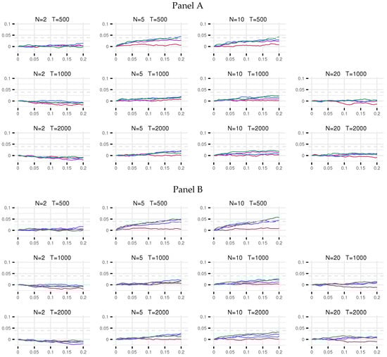
Figure 1. p-Value size discrepancy of the test statistic (15) of orders 1 (red), 2 (purple), 3 (blue), and 4 (green). The test is based on the correctly specified DGP, which is CEC-GARCH with persistence of $0.95$, kurtosis of 4 (Panel A) and 6 (Panel B), and equicorrelation of $0.33$. The dashed line indicates the upper 95% confidence level of $1.96/\sqrt{2500}$.

We move on to the strongly correlated situation, that is, $\rho =0.67$. The size discrepancies are in Figure 2, see also Table A7. The story remains, for most parts, similar to that of the weakly correlated system. Now the test is somewhat oversized when $T=500$ and the Taylor polynomial is at least equal to two. The equicorrelation matrix becomes gradually more ill-conditioned as its dimension grows but is still reasonably accurately inverted when $N=20$.

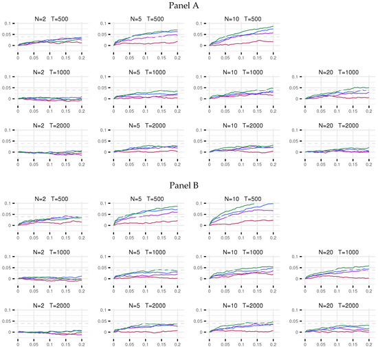
Figure 2. p-Value size discrepancy of the test statistic (15) of orders 1 (red), 2 (purple), 3 (blue), and 4 (green). The test is based on the correctly specified DGP, which is CEC-GARCH with persistence of $0.95$, kurtosis of 4 (Panel A) and 6 (Panel B), and equicorrelation of $0.67$. The dashed line indicates the upper 95% confidence level of $1.96/\sqrt{2500}$.

Furthermore, we consider a situation where we replace the equicorrelation matrix with a positive definite matrix comprised of equicorrelation blocks. The block-equicorrelation structure (Engle and Kelly 2012) imposes different equicorrelations between and within blocks of series. We choose $N=12$ and $N=16$ and blocks of size four. The chosen correlation strengths mimic those of the equicorrelated (weak and strong) levels while maintaining similar condition numbers to ensure fair comparison.1 The only difference in Table A8 compared to the equicorrelation case (Table A6 and Table A7) is that the test is slightly oversized when the order of the polynomial exceeds one.

The remaining results address misspecified GARCH equations. Such misspecification may show up in the covariance as time-variation, even if the correlations happen to be constant. The purpose of these simulations is to find out how well our test is able to detect the resulting time-variation in the eigenvalues.

When $g_{it}$ is time-varying but this variance is ignored, the model is indeed misspecified. In these simulations, the GARCH equations are TV-GARCH equations with ${\delta }_0=1$, ${\delta }_1=3$, $\gamma =20$ and $c=0.5$, with equicorrelation coefficient equal to $0.33$ and $0.67$. The slope parameter ${\gamma }_i$ has been calibrated such that the monotonically increasing $G_i(t/T,{\gamma }_i,c_i)$ remains practically equal to zero until $t/T=0.25$ and (almost) reaches one when $t/T=0.75$. This means that there is a rather mild shift in the (local) unconditional variance in these equations over time, resulting in the amplitude of clusters doubling in size over time. The error covariance matrix is thereby time-varying, whereas the error correlation matrix is constant over time. The reported rejection frequencies in Table A9 indicate that the test detects time-variation even for weakly correlated system (see also Figure 3), and even more so with the correlation of $0.67$ (Table A10), which stresses the importance of specifying the GARCH equations properly before testing constancy of correlations. The rejection frequency increases with the sample size and the dimension of the system, and becomes overwhelming when more information against the null hypothesis becomes available. We also experimented with higher values of ${\delta }_1$, but because the feature is already well illustrated for ${\delta }_1=3,$ we do not report any additional results here.

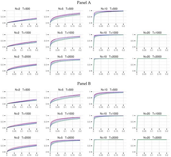
Figure 3. Rejection frequencies of the test statistic (15) of orders 1 to 4. The test is based on CEC-GARCH, while the DGP is TV-CEC-GARCH with persistence of $0.95$, kurtosis of 4 (Panel A) and 6 (Panel B), equicorrelation of $0.33$, and TV-parameters ${\delta }_0=1$, ${\delta }_1=3$, $c=0.5$, and $\gamma =20$ with $s_t=t/T$.

GARCH can also be misspecified such that asymmetry in the form of GJR-GARCH is ignored. The simulation design concerning this sets the ${\alpha }_1=0$ leaving the asymmetric component ${\kappa }_1$ solely responsible for the effect of the past shocks. The parameterisation follows the targets of the previous simulations, that is, the implied kurtosis of four and six, unconditional variance of one and persistence is kept at $0.95$. When the equicorrelation is $0.33$, there is positive size distortion for $N\ge 5$, and for each N, an increase in sample size makes very little difference in terms of improving the size. This is seen from the rejection frequencies reported in Table A11, see also Figure 4. The size distortion is already present when $N=2$ for the $0.67$ equicorrelated case, see Table A12. In situations where the past shocks feed into the volatility via both symmetric and asymmetric channels, the size distortion is milder than in the extreme case discussed here, and will lie somewhere between the results here and those in Table A6 and Table A7. Regardless, it may be concluded that a misspecification in the GARCH equation has a minor impact on constant correlation detection in comparison to the case when the deterministic shift in GARCH is erroneously ignored.

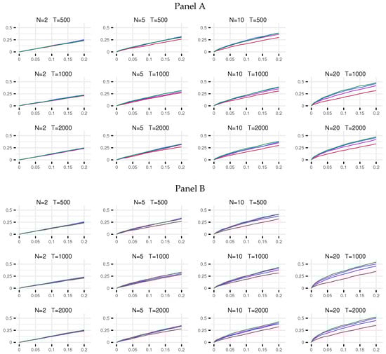
Figure 4. Rejection frequencies of the test statistic (15) of orders 1 (red), 2 (purple), 3 (blue), and 4 (green). The test is based on CEC-GARCH, while the DGP is CEC-GJR-GARCH with persistence of $0.95$, kurtosis of 4 (Panel A) and 6 (Panel B), and equicorrelation of $0.33$.

Yet another type of misspecification occurs when there are volatility spillovers between equations that are ignored while correlations remain constant. To this end we employ an equicorrelation version of the Extended CCC-GARCH (ECCC-GARCH) model of Jeantheau (1998) that use CEC with $\rho =0.33$ and $0.67$. Applications of the ECCC-GARCH model typically involve rather few series, and we therefore limit our simulations to systems of dimension 2, 3, and 5. The first spillover pattern is a circular one, where the past shocks travel from one volatility to another in a sequence through the system. In the second pattern the spillover shock comes from a single series and enters volatility of all the other series. For details, see Appendix C. The results in Table A13 and Table A14 indicate some size distortion which is, as before, larger the stronger the correlation and also increases with the order of the polynomial used in the test. In these simulations the size distortion is of lesser magnitude than what it was in the previous experiment, where the asymmetry of the GARCH was ignored. It can, however, be expected to vary with the strength of the spillover effect.

Finally, Table A15 and Table A16 and Figure 5 show what happens when, instead of normal, the error vectors are t-distributed with $df=5$ and $df=8$. Not accounting for this and assuming that the errors are multinormal, causes positive size distortion. Again, the distortion is not very large compared to what is observed in connection with ignoring the time-variation. It increases when the tails grow fatter (degrees of freedom decrease from eight to five) and when the order of the polynomial in the test grows. It may be noted, however, that this design may not be completely realistic. In practice it is quite possible that the GARCH residuals of equation i may seem to follow a t-distribution just because the GARCH component is misspecified, for example by ignoring the deterministic component $g_{it}$. Here we simulate the case in which the standard GARCH equation with normal errors for some unknown reason does not adequately describe the conditional variances. Once again, these results suggest that the GARCH equations have to be correctly specified before testing constancy of correlations can be attempted.

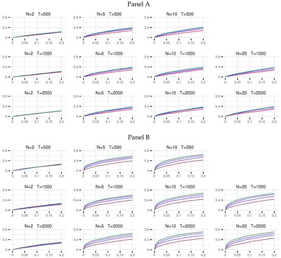
Figure 5. Rejection frequencies of the test statistic (15) of orders 1 (red), 2 (purple), 3 (blue), and 4 (green). The test is based on CEC-GARCH with normal errors, while the DGP has t-distributed errors, with persistence of $0.95$, $df=8$ (Panel A) and $df=5$ (Panel B), and equicorrelation of $0.33$.

It is worth mentioning that when (3) is valid, the error covariance matrix is nonconstant even when the correlations are constant. In that case, the test by Yang (2014) would no doubt reject the null hypothesis of a constant error covariance matrix, whereas our test, after modelling the time-varying error variances, would not reject constancy of the error correlation matrix.

Results of these simulations underline the need of testing adequacy of the GARCH model (constancy, asymmetry spillover effects) before embarking on testing constancy of correlations. There is another very large class of extensions to the standard GARCH model not mentioned yet, namely the GARCH-X model, see Han and Kristensen (2014). Within this class the possibilities of misspecification are almost limitless, and in practice the set of potential exogenous variables has to be restricted by theory considerations. We have therefore refrained from simulating designs involving ignored exogenous variables in the GARCH framework.

7. Application

In order to demonstrate the use of the test we select 26 stocks that have been included in the Dow Jones index during the whole observation period from 2 January 2001 to 31 December 2020 and consider their daily returns. The names, symbols and respective categories of the stocks are listed in Table A1 in Appendix A. We split the observation period into two halves such that the returns from 2001 to the end of 2010 form the first period and the rest belong to the second one. Both samples contain approximately 2500 observations. The first part of the sample includes the periods of turbulence due to the dot-com bubble and GFC, the second is tranquil with a lead-up into the recent Covid-19 events. To perform the tests we first determine the number of transitions in the Multiplicative Time-Varying (MTV) GJR-GARCH equations (it can be zero) using the sequential procedure described in Hall et al. (2021). The 26 estimated GARCH equations (or their $g_{it}$ specification test results) are not reported here, but the plots of the multiplicative component (3) together with the daily returns appear in Figure 6, Figure 7, Figure 8, Figure 9 and Figure 10.

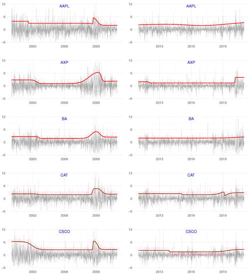
Figure 6. Daily returns of the Dow Jones stocks from Apple (AAPL) to Cisco (CSCO) (grey) and the corresponding deterministic component (red) from the MTV-GJR-GARCH equation for the period 2 January 2001–31 December 2010 (left column) and for 3 January 2011–31 December 2020 (right column).

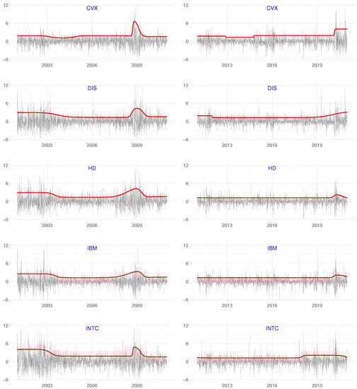
Figure 7. Daily returns of the Dow Jones stocks from Chevron (CVX) to Intel (INTC) (grey) and the corresponding deterministic component (red) from the MTV-GJR-GARCH equation for the period 2 January 2001–31 December 2010 (left column) and for 3 January 2011–31 December 2020 (right column).

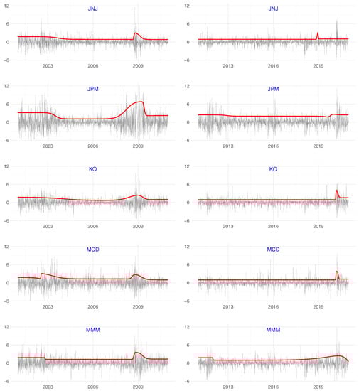
Figure 8. Daily returns of the Dow Jones stocks from Johnson and Johnson (JNJ) to 3M (MMM) (grey) and the corresponding deterministic component (red) from the MTV-GJR-GARCH equation for the period 2 January 2001–31 December 2010 (left column) and for 3 January 2011–31 December 2020 (right column).

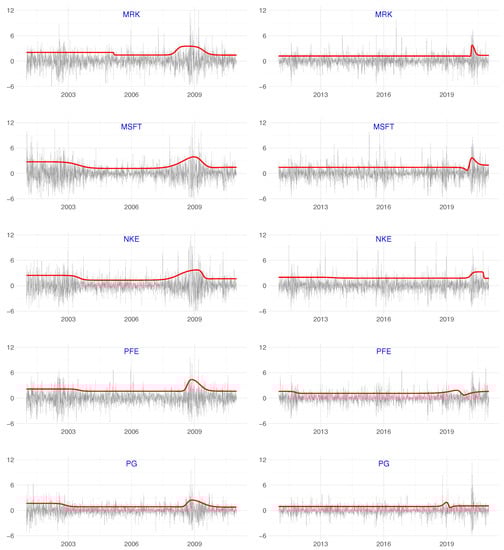
Figure 9. Daily returns of the Dow Jones stocks from Merck (MRK) to Procter & Gamble (PG) (grey) and the corresponding deterministic component (red) from the MTV-GJR-GARCH equation for the period 2 January 2001–31 December 2010 (left column) and for 3 January 2011–31 December 2020 (right column).

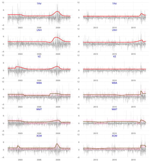
Figure 10. Daily returns of the Dow Jones stocks from Travelers Companies (TRV) to Exxon (XOM) (grey) and the corresponding deterministic component (red) from the MTV-GJR-GARCH equation for the period 2 January 2001–31 December 2010 (left column) and for 3 January 2011–31 December 2020 (right column).

The first-order test clearly rejects the null of constant correlations. Increasing the order of the polynomial in the test statistic does not affect the conclusions. Although the dimension of the null hypothesis increases from 25 to 100, all tests strongly reject the hypothesis of stable correlations for both observation periods. The p-values of the test are practically zero. If this had been attempted for the HST-test, the corresponding degrees of freedom would have increased from 325 to 1300.

While the main purpose of this example is to demonstrate the use of our tests for a relatively large set of stocks, we also consider stability of the pairwise correlations. The magnitudes of the resulting p-values from the pairwise tests applied to the first part of the sample can be found in Table A2 and Table A3 for the polynomial orders of one and two, respectively. Table A4 and Table A5 contain the corresponding ones for the second part of the sample. In the former, the evidence of time-variation in the correlations is very clear. In the latter, there are more cases where the first-order test fails to reject constancy of correlations. The second-order test, however, does find evidence of time-varying correlations between most pairs of stocks. It appears that the change during the second period can often be nonmonotonic rather than monotonic.

This paper clearly demonstrates that our test is the most practical option when the number of assets is large. When it is small so that both tests are available, we can make comparisons and see how much power may be lost when our parsimonious test is applied instead of the HST-test. To this end, groups of three to four stocks are subsequently examined. The results are consistent in most all cases. Two exceptions are discussed next.

The four stocks representing consumer staples (WMT, WBA), services (VZ), and energy (XOM) form the first example. Our test for 2001–2010 results in p-values of 0.0134 and 0.0000 for test orders one (three degrees of freedom, df) and two (six df), respectively. In 2011–2020, the corresponding p-values are 0.1059 and 0.0001. For the HST-test, the p-values for 2001–2010 are 0.0000 for both polynomial orders (six and 12 df), and for 2011–2020 they are 0.0001 and 0.0000, respectively. The obvious conclusion is that the parsimonious test should mainly be used when the other test is no longer applicable.

The three information technology companies AAPL, IBM and INTC, form an example of the smallest collection of stocks such that our test differs from the HST-test. For 2001–2010, the p-values for the first and second-order versions of our tests with two and four df are 0.0103 and 0.0000. The p-values of the corresponding HST-test (three and six df) are 0.0413 and 0.0000. For the second part of the sample, the p-values of our parsimonious test are 0.3459 and 0.0001, compared to 0.0000 for both orders for the HST-test. Here we note the rather rare occasion (2001–2010, first-order test) in which our test is more powerful than its competitor. An explanation may be found in Table A2. It is seen that only one of the p-values of the three pairwise tests lies below $0.1$. Thus, in the HST-test only one pair weighs towards a rejection, whereas the evidence against the null is more spread out in the test based on the eigenvalues, and the test has one df less than the HST-test.

In this example, the alternative to constancy of correlations is that the correlations vary as a function of time. However, both the parsimonious and the HST test are conditioned on the choice of the transition variable which need not be deterministic. This means that they are equally useful for practitioners who may wish to examine correlation stability over some other indicator than time. The underlying theoretical foundations of the tests are unaffected by such considerations, and hence the integrity of the tests is not compromised.

8. Conclusions

In this paper we derive a test for testing constancy of the correlation matrix in the multivariate time-varying GARCH model. It bears some similarity to the test of constancy of the error covariance matrix in a multivariate model by Yang (2014). However, there are substantial differences between the two tests. In Yang’s test, the model for covariances need not be a GARCH model, whereas our test is designed for a class of multivariate GARCH models. It is based on the decomposition of the error covariance matrix into variances and the correlation matrix as in Bollerslev (1990). The advantage of this decomposition is that one can test constancy of the conditional variances one by one as described in Amado and Teräsvirta (2017) or Hall et al. (2021), and estimate the time-varying variances before considering the constancy of correlations. This makes it possible to examine potential nonconstancy in the error correlation matrix such that time-variation in variances has already been taken care of. The simulation results emphasise the importance of correct specification of GARCH equations before constancy of the correlation matrix is tested.

The test is intended for use in situations in which the number of variables, typically asset returns, is large, and where for this reason the test by Hall et al. (2021) is either not available or suffers from numerical problems. Our simulations evidence the test is reasonably well-behaved as long as the conditional variances are correctly specified. The Dow-Jones example illustrates the use of the test in the entire 26-dimensional system, as well as conducting 325 pairwise tests and tests on some selected subgroups. Pairwise tests, while not the main topic of this paper, would help locate those pairs whose correlations are constant. This in turn would help specifying and estimating the final model.

Appendix C.1. Size

Table A6 and Table A7 contain the size simulations, where the DGP is a CEC-GARCH (constant equicorrelation). For each series, $g_t=1$ and the parameterisation of the GARCH equation is such that the persistence is $0.95$ and kurtosis is set to 4 in the first experiment, and to 6 in the second. That is, ${\alpha }_1=0.1104$, ${\beta }_1=0.8396$ in the former, and ${\alpha }_1=0.1561$, ${\beta }_1=0.7939$ for the latter. The GARCH intercept is set to $1-{\alpha }_1-{\beta }_1$ to standardise the unconditional variance to unity. The equicorrelation coefficient is equal to $0.33$ in the former and $0.67$ in the latter. The transition variable in the test is a linear time trend. The dimension N ranges from 2 to 20, and sample size T from 500 to 2000. Note that the smallest size $T=500$ is no longer feasible for $N=20$.

We extend the previous set-up by defining the constant correlation matrix as having a block structure. The system of N series is divided into subgroups consisting of four series. Group i is described as having an equicorrelated state with ${\rho }_i$ as the correlation parameter, $i=1,\dots ,N/4$. The correlation between groups i and j is defined as $\sqrt{{\rho }_i{\rho }_j}$. This structure ensures positive definiteness of the resulting correlation matrix. We consider $N=12$ (three groups of four series), first with $\mathit{\rho }=(0.2,0.3,0.4)$ and then $\mathit{\rho }=(0.25,0.5,0.75)$. The condition numbers of the resulting matrices are similar ($7.13$ and $25.69$) to the ones for equicorrelated matrices of the same dimension with correlation $0.33$ (condition number $C=7$) and $0.67$ (condition number $C=25$), respectively. This is important, because there is an introduced error associated with the matrix inversions that take place during the computation of the test statistic, and the error gets larger the higher the dimension N and the closer the matrix is to singularity. Setting the condition numbers equal will ensure the error is at par across the models and the results are comparable. We further extend the set up to $N=16$ (four groups of four series), with $\mathit{\rho }=(0.10,0.20,0.35,0.45)$ and $\mathit{\rho }=(0.25,0.35,0.55,0.75)$. The condition numbers for these matrices are $9.20$ and $32.21$, again aligning with those of equicorrelated systems of the same size ($C=9$ when $\rho =0.33$, and $C=33$ when $\rho =0.67$). The GARCH parameterisation is the same as in the first experiment, targeting persistence $0.95$ and kurtosis 4 and 6. The simulation results are presented in Table A8.

Appendix C.2. Misspecified Variance

The next experiment investigates the effect of neglecting the TV-component. That is, the DGP is a TV-CEC-GARCH, but the baseline volatility shift is ignored at the estimation stage, and only a CEC-GARCH model is estimated. As before, the GARCH equations are set up with persistence of $0.95$, kurtosis of 4 and 6, ${\alpha }_0=1-{\alpha }_1-{\beta }_1$ for each series, and two strengths of equicorrelation are examined, $0.33$ and $0.67$. The TV-component has a transition located at the center of the sample, and the transition variable is a linear time trend. The speed of the transition is set to $\gamma =20$, which translates to a transition that gradually begins at the first quartile and finishes at the third. The magnitude of the increase in the volatility from the initial level of ${\delta }_0=1$ is set to ${\delta }_1=3$ in the first simulation, and to ${\delta }_1=8$ in the second one, which effectively doubles and triples the standard deviations, respectively. The results for ${\delta }_1=3$ are presented in Table A9 and Table A10. Because the result indicates a very strong tendency to reject the null even at the rather modest increase in variance, the results for ${\delta }_1=8$ are omitted.

Another experiment investigates the sensitivity of the test to the correctness of the GARCH model specification. In this case the GARCH equation is misspecified such that it includes an asymmetry component (GJR-GARCH), but this is ignored when the model is estimated and the test statistic computed. To keep the results comparable, the parameters are chosen such that the implied kurtosis levels are 4 and 6, in addition to keeping the unconditional variance equal to one (${\alpha }_0=1-{\alpha }_1-0.5{\kappa }_1-{\beta }_1$ for each series) and persistence at $0.95$. We choose to look at the extreme case where the effect of the past shock is inherited only from the negative shocks (i.e., ${\alpha }_1=0$). This yields ${\kappa }_1=0.14,$ ${\beta }_1=0.88$ for the case of kurtosis $=4$ and ${\kappa }_1=0.198,{\beta }_1=0.851$ when kurtosis $=6$. The results are tabulated in Table A11 and Table A12 for the two levels of correlation ($0.33$ and $0.67$, respectively).

To investigate the sensitivity of the test to volatility spillovers we use the Extended CEC (ECEC) model which is a special case of the Extended CCC (ECCC) model of Jeantheau (1998). We consider two patterns for the spillover effects for the past shocks (excluding spillovers from past volatilities). First is a circular pattern, where the past shock of the first series enters the next period’s volatility of the second series, the past shock of the second enters the volatility of the third, and so on. The past shock of the last series then enters the volatility of the first series. The second set up is a spillover from a single source to all other series. The parameterisation mimics the earlier simulations in that persistence is set to $0.95$, and kurtosis is 4. That is, ${\beta }_1=0.8396$ and ${\alpha }_1=0.0704$, and the spillover coefficient is $0.04$. For the single source case, the first series has no spillover effect, and thus its ${\alpha }_1=0.1104$. The intercept is again set to $0.05$ for unit conditional variance for each series. For the correlation part we use the CEC models with weak and strong correlations ($\rho =0.33$ and $0.67$, respectively). In practice, the ECCC models are used in low-dimensional applications, and therefore we choose to use $N=2,3,5$. The results are found in Table A13 and Table A14.

Appendix C.3. Misspecified Error Distribution

As the last investigation we look into the effect of nonnormality of the error distribution. We choose t-distribution with $df=8$ and $df=5$. To create multivariate t-distributed data, the individual noise series are first standardised to have unit variance. The correlation matrix is again an equicorrelated one, with $\rho =0.33$ and $\rho =0.67$, as before. The resulting data is thus correlated multivariate t, with t-distributed (standardised) marginals. The GARCH parameters are chosen such that the fourth moment still exists, and the resulting kurtosis is reasonable. We also wish to keep the persistence at $0.95$ to allow for comparison with the normal cases discussed earlier, and the GARCH intercept is set to $1-{\alpha }_1-{\beta }_1$. To this end, we choose ${\alpha }_1=0.06$ and ${\beta }_1=0.89$ when $df=8$ (the implied kurtosis is $5.17$), and ${\alpha }_1=0.03$ and ${\beta }_1=0.92$ for $df=5$ (the implied kurtosis is $9.72$). The results of the size simulations are presented in Table A15 and Table A16.

Table A6. Size of the test. The data is generated from a CEC-GARCH with persistence of $0.95$, kurtosis of 4 (Panel A) and 6 (Panel B), and equicorrelation coefficient of $0.33$. 2500 replications.

			Order 1				Order 2				Order 3				Order 4
$\mathit{N}$	$\mathit{T}$		1%	5%	10%		1%	5%	10%		1%	5%	10%		1%	5%	10%
Panel A
2	500		0.010	0.048	0.108		0.009	0.053	0.102		0.008	0.049	0.107		0.013	0.054	0.099
2	1000		0.012	0.041	0.087		0.010	0.046	0.091		0.012	0.048	0.102		0.009	0.049	0.093
2	2000		0.008	0.045	0.097		0.008	0.047	0.088		0.009	0.045	0.092		0.010	0.046	0.090
5	500		0.013	0.058	0.107		0.015	0.068	0.124		0.019	0.070	0.130		0.017	0.071	0.126
5	1000		0.010	0.051	0.101		0.014	0.052	0.102		0.014	0.060	0.113		0.017	0.057	0.110
5	2000		0.010	0.052	0.103		0.008	0.050	0.107		0.011	0.048	0.106		0.013	0.055	0.109
10	500		0.009	0.050	0.106		0.010	0.062	0.121		0.013	0.070	0.122		0.019	0.064	0.125
10	1000		0.010	0.054	0.101		0.010	0.056	0.107		0.012	0.054	0.118		0.012	0.058	0.108
10	2000		0.010	0.054	0.102		0.012	0.055	0.114		0.014	0.058	0.104		0.014	0.064	0.118
20	1000		0.012	0.050	0.088		0.009	0.052	0.099		0.009	0.052	0.103		0.009	0.051	0.101
20	2000		0.015	0.048	0.094		0.012	0.050	0.103		0.010	0.050	0.100		0.011	0.056	0.107
Panel B
2	500		0.010	0.049	0.104		0.012	0.056	0.104		0.010	0.052	0.106		0.014	0.058	0.102
2	1000		0.012	0.040	0.085		0.010	0.045	0.092		0.012	0.048	0.102		0.009	0.050	0.094
2	2000		0.008	0.045	0.094		0.007	0.048	0.087		0.010	0.044	0.095		0.009	0.044	0.092
5	500		0.013	0.059	0.108		0.018	0.072	0.126		0.020	0.074	0.135		0.021	0.075	0.134
5	1000		0.011	0.050	0.101		0.012	0.051	0.100		0.014	0.056	0.108		0.014	0.053	0.109
5	2000		0.010	0.054	0.102		0.008	0.054	0.110		0.011	0.051	0.110		0.015	0.058	0.108
10	500		0.010	0.053	0.104		0.010	0.066	0.128		0.016	0.076	0.133		0.021	0.072	0.133
10	1000		0.012	0.054	0.104		0.012	0.053	0.108		0.012	0.054	0.116		0.016	0.063	0.112
10	2000		0.010	0.051	0.101		0.012	0.058	0.119		0.016	0.060	0.107		0.016	0.066	0.124
20	1000		0.012	0.050	0.090		0.010	0.052	0.102		0.010	0.055	0.103		0.010	0.054	0.103
20	2000		0.014	0.048	0.093		0.012	0.048	0.107		0.009	0.055	0.101		0.013	0.056	0.116

Table A6. Size of the test. The data is generated from a CEC-GARCH with persistence of $0.95$, kurtosis of 4 (Panel A) and 6 (Panel B), and equicorrelation coefficient of $0.33$. 2500 replications.

			Order 1				Order 2				Order 3				Order 4
$\mathit{N}$	$\mathit{T}$		1%	5%	10%		1%	5%	10%		1%	5%	10%		1%	5%	10%
Panel A
2	500		0.010	0.048	0.108		0.009	0.053	0.102		0.008	0.049	0.107		0.013	0.054	0.099
2	1000		0.012	0.041	0.087		0.010	0.046	0.091		0.012	0.048	0.102		0.009	0.049	0.093
2	2000		0.008	0.045	0.097		0.008	0.047	0.088		0.009	0.045	0.092		0.010	0.046	0.090
5	500		0.013	0.058	0.107		0.015	0.068	0.124		0.019	0.070	0.130		0.017	0.071	0.126
5	1000		0.010	0.051	0.101		0.014	0.052	0.102		0.014	0.060	0.113		0.017	0.057	0.110
5	2000		0.010	0.052	0.103		0.008	0.050	0.107		0.011	0.048	0.106		0.013	0.055	0.109
10	500		0.009	0.050	0.106		0.010	0.062	0.121		0.013	0.070	0.122		0.019	0.064	0.125
10	1000		0.010	0.054	0.101		0.010	0.056	0.107		0.012	0.054	0.118		0.012	0.058	0.108
10	2000		0.010	0.054	0.102		0.012	0.055	0.114		0.014	0.058	0.104		0.014	0.064	0.118
20	1000		0.012	0.050	0.088		0.009	0.052	0.099		0.009	0.052	0.103		0.009	0.051	0.101
20	2000		0.015	0.048	0.094		0.012	0.050	0.103		0.010	0.050	0.100		0.011	0.056	0.107
Panel B
2	500		0.010	0.049	0.104		0.012	0.056	0.104		0.010	0.052	0.106		0.014	0.058	0.102
2	1000		0.012	0.040	0.085		0.010	0.045	0.092		0.012	0.048	0.102		0.009	0.050	0.094
2	2000		0.008	0.045	0.094		0.007	0.048	0.087		0.010	0.044	0.095		0.009	0.044	0.092
5	500		0.013	0.059	0.108		0.018	0.072	0.126		0.020	0.074	0.135		0.021	0.075	0.134
5	1000		0.011	0.050	0.101		0.012	0.051	0.100		0.014	0.056	0.108		0.014	0.053	0.109
5	2000		0.010	0.054	0.102		0.008	0.054	0.110		0.011	0.051	0.110		0.015	0.058	0.108
10	500		0.010	0.053	0.104		0.010	0.066	0.128		0.016	0.076	0.133		0.021	0.072	0.133
10	1000		0.012	0.054	0.104		0.012	0.053	0.108		0.012	0.054	0.116		0.016	0.063	0.112
10	2000		0.010	0.051	0.101		0.012	0.058	0.119		0.016	0.060	0.107		0.016	0.066	0.124
20	1000		0.012	0.050	0.090		0.010	0.052	0.102		0.010	0.055	0.103		0.010	0.054	0.103
20	2000		0.014	0.048	0.093		0.012	0.048	0.107		0.009	0.055	0.101		0.013	0.056	0.116

Table A7. Size of the test. The data is generated from a CEC-GARCH with persistence of $0.95$, kurtosis of 4 (Panel A) and 6 (Panel B), and equicorrelation coefficient of $0.67$. 2500 replications.

			Order 1				Order 2				Order 3				Order 4
$\mathit{N}$	$\mathit{T}$		1%	5%	10%		1%	5%	10%		1%	5%	10%		1%	5%	10%
Panel A
2	500		0.011	0.060	0.112		0.015	0.063	0.124		0.016	0.064	0.124		0.018	0.069	0.117
2	1000		0.010	0.045	0.090		0.013	0.050	0.094		0.013	0.052	0.104		0.013	0.055	0.105
2	2000		0.008	0.048	0.093		0.010	0.048	0.094		0.012	0.043	0.102		0.012	0.048	0.094
5	500		0.016	0.059	0.107		0.023	0.074	0.134		0.026	0.086	0.152		0.028	0.088	0.154
5	1000		0.010	0.053	0.108		0.017	0.060	0.107		0.022	0.067	0.120		0.020	0.070	0.126
5	2000		0.013	0.050	0.102		0.012	0.062	0.116		0.014	0.068	0.120		0.017	0.061	0.128
10	500		0.012	0.056	0.108		0.017	0.075	0.144		0.020	0.079	0.147		0.024	0.089	0.160
10	1000		0.012	0.060	0.116		0.016	0.061	0.120		0.016	0.066	0.126		0.023	0.070	0.129
10	2000		0.014	0.056	0.104		0.012	0.062	0.120		0.014	0.060	0.113		0.017	0.070	0.124
20	1000		0.011	0.056	0.108		0.013	0.063	0.115		0.012	0.065	0.130		0.018	0.072	0.133
20	2000		0.012	0.048	0.104		0.011	0.052	0.108		0.012	0.051	0.107		0.014	0.056	0.113
Panel B
2	500		0.012	0.061	0.112		0.017	0.071	0.128		0.021	0.068	0.130		0.021	0.072	0.126
2	1000		0.010	0.045	0.091		0.013	0.050	0.100		0.013	0.053	0.106		0.012	0.058	0.108
2	2000		0.009	0.048	0.094		0.010	0.050	0.095		0.012	0.049	0.105		0.012	0.050	0.102
5	500		0.017	0.061	0.113		0.025	0.083	0.143		0.031	0.094	0.166		0.036	0.098	0.162
5	1000		0.010	0.053	0.108		0.019	0.063	0.113		0.024	0.071	0.126		0.021	0.075	0.132
5	2000		0.013	0.050	0.102		0.016	0.068	0.122		0.018	0.071	0.128		0.022	0.073	0.138
10	500		0.014	0.056	0.115		0.024	0.086	0.156		0.032	0.100	0.164		0.036	0.113	0.184
10	1000		0.014	0.060	0.118		0.020	0.066	0.121		0.021	0.073	0.135		0.025	0.081	0.145
10	2000		0.015	0.054	0.106		0.016	0.066	0.126		0.018	0.066	0.122		0.020	0.080	0.136
20	1000		0.011	0.060	0.110		0.017	0.068	0.124		0.018	0.071	0.130		0.023	0.079	0.144
20	2000		0.011	0.052	0.102		0.014	0.060	0.118		0.015	0.059	0.119		0.019	0.069	0.128

Table A7. Size of the test. The data is generated from a CEC-GARCH with persistence of $0.95$, kurtosis of 4 (Panel A) and 6 (Panel B), and equicorrelation coefficient of $0.67$. 2500 replications.

			Order 1				Order 2				Order 3				Order 4
$\mathit{N}$	$\mathit{T}$		1%	5%	10%		1%	5%	10%		1%	5%	10%		1%	5%	10%
Panel A
2	500		0.011	0.060	0.112		0.015	0.063	0.124		0.016	0.064	0.124		0.018	0.069	0.117
2	1000		0.010	0.045	0.090		0.013	0.050	0.094		0.013	0.052	0.104		0.013	0.055	0.105
2	2000		0.008	0.048	0.093		0.010	0.048	0.094		0.012	0.043	0.102		0.012	0.048	0.094
5	500		0.016	0.059	0.107		0.023	0.074	0.134		0.026	0.086	0.152		0.028	0.088	0.154
5	1000		0.010	0.053	0.108		0.017	0.060	0.107		0.022	0.067	0.120		0.020	0.070	0.126
5	2000		0.013	0.050	0.102		0.012	0.062	0.116		0.014	0.068	0.120		0.017	0.061	0.128
10	500		0.012	0.056	0.108		0.017	0.075	0.144		0.020	0.079	0.147		0.024	0.089	0.160
10	1000		0.012	0.060	0.116		0.016	0.061	0.120		0.016	0.066	0.126		0.023	0.070	0.129
10	2000		0.014	0.056	0.104		0.012	0.062	0.120		0.014	0.060	0.113		0.017	0.070	0.124
20	1000		0.011	0.056	0.108		0.013	0.063	0.115		0.012	0.065	0.130		0.018	0.072	0.133
20	2000		0.012	0.048	0.104		0.011	0.052	0.108		0.012	0.051	0.107		0.014	0.056	0.113
Panel B
2	500		0.012	0.061	0.112		0.017	0.071	0.128		0.021	0.068	0.130		0.021	0.072	0.126
2	1000		0.010	0.045	0.091		0.013	0.050	0.100		0.013	0.053	0.106		0.012	0.058	0.108
2	2000		0.009	0.048	0.094		0.010	0.050	0.095		0.012	0.049	0.105		0.012	0.050	0.102
5	500		0.017	0.061	0.113		0.025	0.083	0.143		0.031	0.094	0.166		0.036	0.098	0.162
5	1000		0.010	0.053	0.108		0.019	0.063	0.113		0.024	0.071	0.126		0.021	0.075	0.132
5	2000		0.013	0.050	0.102		0.016	0.068	0.122		0.018	0.071	0.128		0.022	0.073	0.138
10	500		0.014	0.056	0.115		0.024	0.086	0.156		0.032	0.100	0.164		0.036	0.113	0.184
10	1000		0.014	0.060	0.118		0.020	0.066	0.121		0.021	0.073	0.135		0.025	0.081	0.145
10	2000		0.015	0.054	0.106		0.016	0.066	0.126		0.018	0.066	0.122		0.020	0.080	0.136
20	1000		0.011	0.060	0.110		0.017	0.068	0.124		0.018	0.071	0.130		0.023	0.079	0.144
20	2000		0.011	0.052	0.102		0.014	0.060	0.118		0.015	0.059	0.119		0.019	0.069	0.128

Table A8. Size of the test. The data is generated from a block-correlation-GARCH with persistence of $0.95$, kurtosis of 4 (Panel A) and 6 (Panel B). The condition numbers (C) in the top and bottom section of each panel correspond to a weak and strong correlation, respectively. 2500 replications.

			Order 1				Order 2				Order 3				Order 4
$\mathit{N}$	$\mathit{T}$	$\mathit{C}$	1%	5%	10%		1%	5%	10%		1%	5%	10%		1%	5%	10%
Panel A
12	1000	7.13	0.013	0.058	0.116		0.014	0.058	0.117		0.012	0.062	0.117		0.015	0.064	0.120
12	2000	7.13	0.009	0.054	0.100		0.011	0.051	0.108		0.015	0.060	0.111		0.018	0.064	0.119
16	1000	9.20	0.013	0.053	0.114		0.019	0.064	0.125		0.014	0.062	0.122		0.014	0.063	0.126
16	2000	9.20	0.010	0.052	0.109		0.014	0.064	0.119		0.010	0.068	0.118		0.018	0.067	0.121
12	1000	25.69	0.015	0.062	0.111		0.019	0.072	0.139		0.022	0.074	0.132		0.022	0.075	0.138
12	2000	25.69	0.010	0.052	0.103		0.017	0.063	0.124		0.012	0.075	0.125		0.020	0.075	0.135
16	1000	32.21	0.009	0.060	0.120		0.015	0.070	0.128		0.017	0.073	0.130		0.017	0.076	0.138
16	2000	32.21	0.010	0.055	0.112		0.014	0.071	0.116		0.011	0.069	0.124		0.016	0.070	0.133
Panel B
12	1000	7.13	0.013	0.059	0.118		0.016	0.064	0.122		0.014	0.066	0.126		0.016	0.068	0.122
12	2000	7.13	0.008	0.053	0.098		0.014	0.064	0.116		0.018	0.064	0.122		0.027	0.076	0.132
16	1000	9.20	0.014	0.058	0.114		0.021	0.070	0.130		0.017	0.074	0.129		0.016	0.068	0.134
16	2000	9.20	0.010	0.053	0.107		0.017	0.070	0.129		0.013	0.075	0.124		0.024	0.078	0.136
12	1000	25.69	0.014	0.064	0.114		0.020	0.079	0.141		0.024	0.080	0.142		0.029	0.084	0.150
12	2000	25.69	0.011	0.053	0.107		0.020	0.069	0.140		0.016	0.081	0.136		0.029	0.089	0.159
16	1000	32.21	0.008	0.060	0.120		0.021	0.076	0.138		0.019	0.081	0.140		0.023	0.087	0.149
16	2000	32.21	0.011	0.058	0.114		0.021	0.079	0.134		0.017	0.076	0.138		0.028	0.093	0.157

Table A8. Size of the test. The data is generated from a block-correlation-GARCH with persistence of $0.95$, kurtosis of 4 (Panel A) and 6 (Panel B). The condition numbers (C) in the top and bottom section of each panel correspond to a weak and strong correlation, respectively. 2500 replications.

			Order 1				Order 2				Order 3				Order 4
$\mathit{N}$	$\mathit{T}$	$\mathit{C}$	1%	5%	10%		1%	5%	10%		1%	5%	10%		1%	5%	10%
Panel A
12	1000	7.13	0.013	0.058	0.116		0.014	0.058	0.117		0.012	0.062	0.117		0.015	0.064	0.120
12	2000	7.13	0.009	0.054	0.100		0.011	0.051	0.108		0.015	0.060	0.111		0.018	0.064	0.119
16	1000	9.20	0.013	0.053	0.114		0.019	0.064	0.125		0.014	0.062	0.122		0.014	0.063	0.126
16	2000	9.20	0.010	0.052	0.109		0.014	0.064	0.119		0.010	0.068	0.118		0.018	0.067	0.121
12	1000	25.69	0.015	0.062	0.111		0.019	0.072	0.139		0.022	0.074	0.132		0.022	0.075	0.138
12	2000	25.69	0.010	0.052	0.103		0.017	0.063	0.124		0.012	0.075	0.125		0.020	0.075	0.135
16	1000	32.21	0.009	0.060	0.120		0.015	0.070	0.128		0.017	0.073	0.130		0.017	0.076	0.138
16	2000	32.21	0.010	0.055	0.112		0.014	0.071	0.116		0.011	0.069	0.124		0.016	0.070	0.133
Panel B
12	1000	7.13	0.013	0.059	0.118		0.016	0.064	0.122		0.014	0.066	0.126		0.016	0.068	0.122
12	2000	7.13	0.008	0.053	0.098		0.014	0.064	0.116		0.018	0.064	0.122		0.027	0.076	0.132
16	1000	9.20	0.014	0.058	0.114		0.021	0.070	0.130		0.017	0.074	0.129		0.016	0.068	0.134
16	2000	9.20	0.010	0.053	0.107		0.017	0.070	0.129		0.013	0.075	0.124		0.024	0.078	0.136
12	1000	25.69	0.014	0.064	0.114		0.020	0.079	0.141		0.024	0.080	0.142		0.029	0.084	0.150
12	2000	25.69	0.011	0.053	0.107		0.020	0.069	0.140		0.016	0.081	0.136		0.029	0.089	0.159
16	1000	32.21	0.008	0.060	0.120		0.021	0.076	0.138		0.019	0.081	0.140		0.023	0.087	0.149
16	2000	32.21	0.011	0.058	0.114		0.021	0.079	0.134		0.017	0.076	0.138		0.028	0.093	0.157

Table A9. Rejection frequencies: misspecified deterministic variance component. The data is generated from a TV-CEC-GARCH with the GARCH equation parameterised such that persistence is $0.95$ and kurtosis is 4 (Panel A) and 6 (Panel B), and the TV-component has ${\delta }_0=1$, ${\delta }_1=3$, $c=0.5$ and $\gamma =20$, and equicorrelation coefficient of $0.33$. The test ignores the TV-component. 2500 replications.

			Order 1				Order 2				Order 3				Order 4
$\mathit{N}$	$\mathit{T}$		1%	5%	10%		1%	5%	10%		1%	5%	10%		1%	5%	10%
Panel A
2	500		0.052	0.148	0.241		0.037	0.134	0.229		0.030	0.112	0.199		0.031	0.091	0.178
2	1000		0.072	0.209	0.316		0.053	0.173	0.289		0.043	0.140	0.239		0.039	0.127	0.209
2	2000		0.125	0.307	0.417		0.095	0.253	0.376		0.079	0.218	0.336		0.064	0.195	0.297
5	500		0.293	0.517	0.630		0.310	0.559	0.680		0.221	0.450	0.590		0.168	0.368	0.514
5	1000		0.486	0.680	0.775		0.452	0.680	0.776		0.343	0.583	0.703		0.280	0.500	0.630
5	2000		0.718	0.862	0.915		0.678	0.849	0.911		0.595	0.782	0.862		0.517	0.719	0.808
10	500		0.768	0.894	0.928		0.861	0.954	0.972		0.762	0.902	0.951		0.651	0.842	0.902
10	1000		0.914	0.959	0.976		0.942	0.981	0.990		0.884	0.960	0.978		0.810	0.927	0.959
10	2000		0.990	0.995	0.998		0.990	0.997	0.999		0.980	0.993	0.997		0.963	0.989	0.995
20	1000		0.999	1.000	1.000		1.000	1.000	1.000		1.000	1.000	1.000		0.998	1.000	1.000
20	2000		1.000	1.000	1.000		1.000	1.000	1.000		1.000	1.000	1.000		1.000	1.000	1.000
Panel B
2	500		0.050	0.141	0.228		0.036	0.123	0.211		0.028	0.104	0.186		0.028	0.083	0.164
2	1000		0.075	0.214	0.320		0.053	0.170	0.282		0.044	0.140	0.238		0.038	0.129	0.204
2	2000		0.146	0.340	0.458		0.109	0.274	0.400		0.093	0.241	0.361		0.075	0.219	0.326
5	500		0.276	0.490	0.604		0.254	0.486	0.615		0.183	0.383	0.524		0.137	0.316	0.448
5	1000		0.498	0.708	0.785		0.421	0.664	0.761		0.331	0.569	0.687		0.272	0.481	0.622
5	2000		0.802	0.913	0.948		0.752	0.893	0.939		0.675	0.844	0.906		0.602	0.789	0.856
10	500		0.746	0.880	0.921		0.779	0.916	0.956		0.652	0.835	0.903		0.554	0.763	0.846
10	1000		0.928	0.970	0.984		0.936	0.976	0.988		0.864	0.952	0.972		0.792	0.914	0.954
10	2000		0.996	1.000	1.000		0.996	0.999	0.999		0.991	0.998	0.999		0.984	0.997	0.998
20	1000		0.999	1.000	1.000		1.000	1.000	1.000		1.000	1.000	1.000		0.995	1.000	1.000
20	2000		1.000	1.000	1.000		1.000	1.000	1.000		1.000	1.000	1.000		1.000	1.000	1.000

Table A9. Rejection frequencies: misspecified deterministic variance component. The data is generated from a TV-CEC-GARCH with the GARCH equation parameterised such that persistence is $0.95$ and kurtosis is 4 (Panel A) and 6 (Panel B), and the TV-component has ${\delta }_0=1$, ${\delta }_1=3$, $c=0.5$ and $\gamma =20$, and equicorrelation coefficient of $0.33$. The test ignores the TV-component. 2500 replications.

			Order 1				Order 2				Order 3				Order 4
$\mathit{N}$	$\mathit{T}$		1%	5%	10%		1%	5%	10%		1%	5%	10%		1%	5%	10%
Panel A
2	500		0.052	0.148	0.241		0.037	0.134	0.229		0.030	0.112	0.199		0.031	0.091	0.178
2	1000		0.072	0.209	0.316		0.053	0.173	0.289		0.043	0.140	0.239		0.039	0.127	0.209
2	2000		0.125	0.307	0.417		0.095	0.253	0.376		0.079	0.218	0.336		0.064	0.195	0.297
5	500		0.293	0.517	0.630		0.310	0.559	0.680		0.221	0.450	0.590		0.168	0.368	0.514
5	1000		0.486	0.680	0.775		0.452	0.680	0.776		0.343	0.583	0.703		0.280	0.500	0.630
5	2000		0.718	0.862	0.915		0.678	0.849	0.911		0.595	0.782	0.862		0.517	0.719	0.808
10	500		0.768	0.894	0.928		0.861	0.954	0.972		0.762	0.902	0.951		0.651	0.842	0.902
10	1000		0.914	0.959	0.976		0.942	0.981	0.990		0.884	0.960	0.978		0.810	0.927	0.959
10	2000		0.990	0.995	0.998		0.990	0.997	0.999		0.980	0.993	0.997		0.963	0.989	0.995
20	1000		0.999	1.000	1.000		1.000	1.000	1.000		1.000	1.000	1.000		0.998	1.000	1.000
20	2000		1.000	1.000	1.000		1.000	1.000	1.000		1.000	1.000	1.000		1.000	1.000	1.000
Panel B
2	500		0.050	0.141	0.228		0.036	0.123	0.211		0.028	0.104	0.186		0.028	0.083	0.164
2	1000		0.075	0.214	0.320		0.053	0.170	0.282		0.044	0.140	0.238		0.038	0.129	0.204
2	2000		0.146	0.340	0.458		0.109	0.274	0.400		0.093	0.241	0.361		0.075	0.219	0.326
5	500		0.276	0.490	0.604		0.254	0.486	0.615		0.183	0.383	0.524		0.137	0.316	0.448
5	1000		0.498	0.708	0.785		0.421	0.664	0.761		0.331	0.569	0.687		0.272	0.481	0.622
5	2000		0.802	0.913	0.948		0.752	0.893	0.939		0.675	0.844	0.906		0.602	0.789	0.856
10	500		0.746	0.880	0.921		0.779	0.916	0.956		0.652	0.835	0.903		0.554	0.763	0.846
10	1000		0.928	0.970	0.984		0.936	0.976	0.988		0.864	0.952	0.972		0.792	0.914	0.954
10	2000		0.996	1.000	1.000		0.996	0.999	0.999		0.991	0.998	0.999		0.984	0.997	0.998
20	1000		0.999	1.000	1.000		1.000	1.000	1.000		1.000	1.000	1.000		0.995	1.000	1.000
20	2000		1.000	1.000	1.000		1.000	1.000	1.000		1.000	1.000	1.000		1.000	1.000	1.000

Table A10. Rejection frequencies: misspecified deterministic variance component. The data is generated from a TV-CEC-GARCH with the GARCH equation parameterised such that persistence is $0.95$ and kurtosis is 4 (Panel A) and 6 (Panel B), and the TV-component has ${\delta }_0=1$, ${\delta }_1=3$, $c=0.5$ and $\gamma =20$, and equicorrelation coefficient of $0.67$. The test ignores the TV-component. 2500 replications.

			Order 1				Order 2				Order 3				Order 4
$\mathit{N}$	$\mathit{T}$		1%	5%	10%		1%	5%	10%		1%	5%	10%		1%	5%	10%
Panel A
2	500		0.227	0.430	0.537		0.226	0.465	0.600		0.182	0.405	0.547		0.158	0.353	0.488
2	1000		0.342	0.547	0.664		0.328	0.568	0.677		0.284	0.521	0.642		0.242	0.464	0.601
2	2000		0.502	0.699	0.777		0.486	0.698	0.790		0.449	0.645	0.750		0.413	0.612	0.712
5	500		0.688	0.828	0.876		0.818	0.924	0.955		0.764	0.901	0.942		0.695	0.860	0.919
5	1000		0.819	0.900	0.930		0.883	0.948	0.969		0.843	0.936	0.962		0.800	0.911	0.952
5	2000		0.941	0.973	0.983		0.962	0.985	0.991		0.944	0.978	0.987		0.919	0.972	0.983
10	500		0.890	0.934	0.955		0.974	0.993	0.995		0.964	0.988	0.996		0.948	0.984	0.990
10	1000		0.948	0.974	0.980		0.988	0.994	0.997		0.982	0.994	0.996		0.973	0.992	0.995
10	2000		0.991	0.994	0.996		0.996	0.999	0.999		0.995	0.999	0.999		0.991	0.997	0.998
20	1000		0.986	0.994	0.998		0.998	1.000	1.000		0.998	0.999	1.000		0.999	0.999	1.000
20	2000		0.999	1.000	1.000		1.000	1.000	1.000		1.000	1.000	1.000		1.000	1.000	1.000
Panel B
2	500		0.200	0.411	0.521		0.185	0.415	0.542		0.154	0.356	0.491		0.128	0.302	0.433
2	1000		0.345	0.556	0.672		0.308	0.548	0.657		0.270	0.506	0.620		0.235	0.445	0.582
2	2000		0.571	0.754	0.826		0.524	0.735	0.823		0.494	0.693	0.790		0.461	0.656	0.752
5	500		0.668	0.816	0.871		0.743	0.883	0.929		0.668	0.842	0.902		0.598	0.794	0.871
5	1000		0.836	0.913	0.942		0.868	0.939	0.962		0.816	0.916	0.950		0.780	0.894	0.934
5	2000		0.975	0.986	0.990		0.977	0.991	0.995		0.966	0.986	0.992		0.951	0.983	0.991
10	500		0.884	0.934	0.954		0.956	0.981	0.991		0.936	0.976	0.986		0.903	0.961	0.981
10	1000		0.957	0.979	0.984		0.982	0.992	0.996		0.974	0.990	0.994		0.960	0.987	0.991
10	2000		0.996	0.998	0.999		0.999	1.000	1.000		0.998	0.999	0.999		0.996	0.998	0.999
20	1000		0.992	0.998	0.999		0.999	1.000	1.000		0.997	1.000	1.000		0.997	0.999	1.000
20	2000		1.000	1.000	1.000		1.000	1.000	1.000		1.000	1.000	1.000		1.000	1.000	1.000

Table A10. Rejection frequencies: misspecified deterministic variance component. The data is generated from a TV-CEC-GARCH with the GARCH equation parameterised such that persistence is $0.95$ and kurtosis is 4 (Panel A) and 6 (Panel B), and the TV-component has ${\delta }_0=1$, ${\delta }_1=3$, $c=0.5$ and $\gamma =20$, and equicorrelation coefficient of $0.67$. The test ignores the TV-component. 2500 replications.

			Order 1				Order 2				Order 3				Order 4
$\mathit{N}$	$\mathit{T}$		1%	5%	10%		1%	5%	10%		1%	5%	10%		1%	5%	10%
Panel A
2	500		0.227	0.430	0.537		0.226	0.465	0.600		0.182	0.405	0.547		0.158	0.353	0.488
2	1000		0.342	0.547	0.664		0.328	0.568	0.677		0.284	0.521	0.642		0.242	0.464	0.601
2	2000		0.502	0.699	0.777		0.486	0.698	0.790		0.449	0.645	0.750		0.413	0.612	0.712
5	500		0.688	0.828	0.876		0.818	0.924	0.955		0.764	0.901	0.942		0.695	0.860	0.919
5	1000		0.819	0.900	0.930		0.883	0.948	0.969		0.843	0.936	0.962		0.800	0.911	0.952
5	2000		0.941	0.973	0.983		0.962	0.985	0.991		0.944	0.978	0.987		0.919	0.972	0.983
10	500		0.890	0.934	0.955		0.974	0.993	0.995		0.964	0.988	0.996		0.948	0.984	0.990
10	1000		0.948	0.974	0.980		0.988	0.994	0.997		0.982	0.994	0.996		0.973	0.992	0.995
10	2000		0.991	0.994	0.996		0.996	0.999	0.999		0.995	0.999	0.999		0.991	0.997	0.998
20	1000		0.986	0.994	0.998		0.998	1.000	1.000		0.998	0.999	1.000		0.999	0.999	1.000
20	2000		0.999	1.000	1.000		1.000	1.000	1.000		1.000	1.000	1.000		1.000	1.000	1.000
Panel B
2	500		0.200	0.411	0.521		0.185	0.415	0.542		0.154	0.356	0.491		0.128	0.302	0.433
2	1000		0.345	0.556	0.672		0.308	0.548	0.657		0.270	0.506	0.620		0.235	0.445	0.582
2	2000		0.571	0.754	0.826		0.524	0.735	0.823		0.494	0.693	0.790		0.461	0.656	0.752
5	500		0.668	0.816	0.871		0.743	0.883	0.929		0.668	0.842	0.902		0.598	0.794	0.871
5	1000		0.836	0.913	0.942		0.868	0.939	0.962		0.816	0.916	0.950		0.780	0.894	0.934
5	2000		0.975	0.986	0.990		0.977	0.991	0.995		0.966	0.986	0.992		0.951	0.983	0.991
10	500		0.884	0.934	0.954		0.956	0.981	0.991		0.936	0.976	0.986		0.903	0.961	0.981
10	1000		0.957	0.979	0.984		0.982	0.992	0.996		0.974	0.990	0.994		0.960	0.987	0.991
10	2000		0.996	0.998	0.999		0.999	1.000	1.000		0.998	0.999	0.999		0.996	0.998	0.999
20	1000		0.992	0.998	0.999		0.999	1.000	1.000		0.997	1.000	1.000		0.997	0.999	1.000
20	2000		1.000	1.000	1.000		1.000	1.000	1.000		1.000	1.000	1.000		1.000	1.000	1.000

Table A11. Rejection frequencies: misspecified GARCH equation. The data is generated from a CEC-GJR-GARCH with the GJR-GARCH equation parameterised such that persistence is $0.95$ and kurtosis is 4 (Panel A) and 6 (Panel B), and equicorrelation coefficient of $0.33$. The test ignores the asymmetric GJR-component. 2500 replications.

			Order 1				Order 2				Order 3				Order 4
$\mathit{N}$	$\mathit{T}$		1%	5%	10%		1%	5%	10%		1%	5%	10%		1%	5%	10%
Panel A
2	500		0.010	0.054	0.104		0.011	0.056	0.113		0.011	0.054	0.109		0.012	0.054	0.109
2	1000		0.012	0.052	0.094		0.011	0.047	0.092		0.015	0.056	0.106		0.014	0.052	0.098
2	2000		0.009	0.053	0.103		0.011	0.049	0.100		0.010	0.052	0.109		0.009	0.051	0.112
5	500		0.018	0.071	0.120		0.025	0.082	0.149		0.028	0.089	0.149		0.028	0.090	0.156
5	1000		0.016	0.069	0.131		0.020	0.080	0.143		0.024	0.086	0.155		0.024	0.093	0.157
5	2000		0.017	0.064	0.134		0.015	0.079	0.147		0.019	0.086	0.157		0.022	0.083	0.153
10	500		0.022	0.089	0.146		0.032	0.113	0.197		0.038	0.126	0.209		0.034	0.117	0.199
10	1000		0.024	0.090	0.151		0.029	0.106	0.179		0.031	0.110	0.197		0.035	0.116	0.198
10	2000		0.019	0.082	0.144		0.029	0.101	0.182		0.030	0.114	0.188		0.039	0.124	0.210
20	1000		0.030	0.094	0.155		0.046	0.137	0.228		0.058	0.168	0.267		0.061	0.179	0.285
20	2000		0.034	0.106	0.170		0.049	0.155	0.236		0.058	0.160	0.261		0.063	0.178	0.274
Panel B
2	500		0.011	0.056	0.105		0.012	0.056	0.116		0.013	0.056	0.109		0.014	0.057	0.109
2	1000		0.011	0.054	0.094		0.012	0.050	0.095		0.016	0.060	0.109		0.016	0.054	0.101
2	2000		0.012	0.055	0.105		0.012	0.051	0.104		0.012	0.056	0.112		0.009	0.055	0.115
5	500		0.020	0.076	0.130		0.024	0.088	0.156		0.030	0.098	0.163		0.032	0.100	0.169
5	1000		0.020	0.073	0.134		0.023	0.087	0.152		0.026	0.093	0.166		0.026	0.099	0.169
5	2000		0.017	0.071	0.140		0.016	0.086	0.158		0.025	0.094	0.170		0.026	0.094	0.169
10	500		0.025	0.090	0.156		0.038	0.123	0.210		0.044	0.138	0.232		0.034	0.133	0.222
10	1000		0.032	0.096	0.164		0.035	0.118	0.203		0.036	0.130	0.220		0.044	0.139	0.225
10	2000		0.026	0.089	0.153		0.039	0.119	0.196		0.040	0.129	0.210		0.053	0.148	0.231
20	1000		0.035	0.102	0.170		0.054	0.166	0.257		0.073	0.192	0.293		0.080	0.214	0.314
20	2000		0.040	0.114	0.188		0.065	0.169	0.259		0.078	0.201	0.293		0.086	0.215	0.313

Table A11. Rejection frequencies: misspecified GARCH equation. The data is generated from a CEC-GJR-GARCH with the GJR-GARCH equation parameterised such that persistence is $0.95$ and kurtosis is 4 (Panel A) and 6 (Panel B), and equicorrelation coefficient of $0.33$. The test ignores the asymmetric GJR-component. 2500 replications.

			Order 1				Order 2				Order 3				Order 4
$\mathit{N}$	$\mathit{T}$		1%	5%	10%		1%	5%	10%		1%	5%	10%		1%	5%	10%
Panel A
2	500		0.010	0.054	0.104		0.011	0.056	0.113		0.011	0.054	0.109		0.012	0.054	0.109
2	1000		0.012	0.052	0.094		0.011	0.047	0.092		0.015	0.056	0.106		0.014	0.052	0.098
2	2000		0.009	0.053	0.103		0.011	0.049	0.100		0.010	0.052	0.109		0.009	0.051	0.112
5	500		0.018	0.071	0.120		0.025	0.082	0.149		0.028	0.089	0.149		0.028	0.090	0.156
5	1000		0.016	0.069	0.131		0.020	0.080	0.143		0.024	0.086	0.155		0.024	0.093	0.157
5	2000		0.017	0.064	0.134		0.015	0.079	0.147		0.019	0.086	0.157		0.022	0.083	0.153
10	500		0.022	0.089	0.146		0.032	0.113	0.197		0.038	0.126	0.209		0.034	0.117	0.199
10	1000		0.024	0.090	0.151		0.029	0.106	0.179		0.031	0.110	0.197		0.035	0.116	0.198
10	2000		0.019	0.082	0.144		0.029	0.101	0.182		0.030	0.114	0.188		0.039	0.124	0.210
20	1000		0.030	0.094	0.155		0.046	0.137	0.228		0.058	0.168	0.267		0.061	0.179	0.285
20	2000		0.034	0.106	0.170		0.049	0.155	0.236		0.058	0.160	0.261		0.063	0.178	0.274
Panel B
2	500		0.011	0.056	0.105		0.012	0.056	0.116		0.013	0.056	0.109		0.014	0.057	0.109
2	1000		0.011	0.054	0.094		0.012	0.050	0.095		0.016	0.060	0.109		0.016	0.054	0.101
2	2000		0.012	0.055	0.105		0.012	0.051	0.104		0.012	0.056	0.112		0.009	0.055	0.115
5	500		0.020	0.076	0.130		0.024	0.088	0.156		0.030	0.098	0.163		0.032	0.100	0.169
5	1000		0.020	0.073	0.134		0.023	0.087	0.152		0.026	0.093	0.166		0.026	0.099	0.169
5	2000		0.017	0.071	0.140		0.016	0.086	0.158		0.025	0.094	0.170		0.026	0.094	0.169
10	500		0.025	0.090	0.156		0.038	0.123	0.210		0.044	0.138	0.232		0.034	0.133	0.222
10	1000		0.032	0.096	0.164		0.035	0.118	0.203		0.036	0.130	0.220		0.044	0.139	0.225
10	2000		0.026	0.089	0.153		0.039	0.119	0.196		0.040	0.129	0.210		0.053	0.148	0.231
20	1000		0.035	0.102	0.170		0.054	0.166	0.257		0.073	0.192	0.293		0.080	0.214	0.314
20	2000		0.040	0.114	0.188		0.065	0.169	0.259		0.078	0.201	0.293		0.086	0.215	0.313

Table A12. Rejection frequencies: misspecified GARCH equation. The data is generated from a CEC-GJR-GARCH with the GJR-GARCH equation parameterised such that persistence is $0.95$ and kurtosis is 4 (Panel A) and 6 (Panel B), and equicorrelation coefficient of $0.67$. The test ignores the asymmetric GJR-component. 2500 replications.

			Order 1				Order 2				Order 3				Order 4
$\mathit{N}$	$\mathit{T}$		1%	5%	10%		1%	5%	10%		1%	5%	10%		1%	5%	10%
Panel A
2	500		0.020	0.078	0.138		0.022	0.096	0.168		0.028	0.102	0.183		0.033	0.111	0.183
2	1000		0.019	0.064	0.120		0.021	0.077	0.135		0.026	0.092	0.155		0.024	0.086	0.156
2	2000		0.020	0.078	0.127		0.020	0.080	0.152		0.024	0.088	0.158		0.022	0.097	0.172
5	500		0.044	0.118	0.190		0.066	0.166	0.264		0.080	0.190	0.279		0.084	0.198	0.298
5	1000		0.036	0.107	0.182		0.048	0.150	0.232		0.074	0.183	0.270		0.078	0.192	0.291
5	2000		0.027	0.109	0.187		0.047	0.142	0.241		0.059	0.168	0.274		0.072	0.185	0.293
10	500		0.066	0.164	0.233		0.108	0.246	0.345		0.137	0.287	0.391		0.145	0.306	0.416
10	1000		0.063	0.151	0.236		0.094	0.234	0.338		0.127	0.274	0.380		0.134	0.304	0.414
10	2000		0.061	0.152	0.227		0.084	0.213	0.303		0.110	0.250	0.361		0.137	0.290	0.395
20	1000		0.091	0.192	0.272		0.152	0.304	0.406		0.200	0.366	0.468		0.236	0.412	0.511
20	2000		0.097	0.194	0.267		0.158	0.301	0.398		0.196	0.358	0.472		0.229	0.406	0.526
Panel B
2	500		0.021	0.082	0.140		0.026	0.102	0.184		0.032	0.112	0.194		0.036	0.120	0.197
2	1000		0.020	0.069	0.124		0.023	0.082	0.146		0.029	0.102	0.164		0.029	0.100	0.170
2	2000		0.022	0.083	0.138		0.023	0.090	0.158		0.029	0.106	0.173		0.027	0.111	0.189
5	500		0.048	0.124	0.202		0.074	0.196	0.286		0.093	0.216	0.317		0.103	0.231	0.334
5	1000		0.040	0.119	0.199		0.062	0.170	0.252		0.089	0.208	0.305		0.100	0.225	0.321
5	2000		0.033	0.123	0.201		0.058	0.165	0.266		0.076	0.198	0.304		0.088	0.219	0.326
10	500		0.078	0.179	0.250		0.131	0.277	0.381		0.172	0.329	0.439		0.176	0.358	0.480
10	1000		0.075	0.175	0.257		0.122	0.271	0.374		0.163	0.314	0.422		0.180	0.350	0.468
10	2000		0.074	0.171	0.252		0.105	0.246	0.343		0.138	0.298	0.411		0.174	0.336	0.457
20	1000		0.108	0.220	0.308		0.193	0.344	0.450		0.250	0.424	0.532		0.301	0.485	0.596
20	2000		0.116	0.223	0.304		0.194	0.341	0.437		0.245	0.426	0.531		0.300	0.485	0.591

Table A12. Rejection frequencies: misspecified GARCH equation. The data is generated from a CEC-GJR-GARCH with the GJR-GARCH equation parameterised such that persistence is $0.95$ and kurtosis is 4 (Panel A) and 6 (Panel B), and equicorrelation coefficient of $0.67$. The test ignores the asymmetric GJR-component. 2500 replications.

			Order 1				Order 2				Order 3				Order 4
$\mathit{N}$	$\mathit{T}$		1%	5%	10%		1%	5%	10%		1%	5%	10%		1%	5%	10%
Panel A
2	500		0.020	0.078	0.138		0.022	0.096	0.168		0.028	0.102	0.183		0.033	0.111	0.183
2	1000		0.019	0.064	0.120		0.021	0.077	0.135		0.026	0.092	0.155		0.024	0.086	0.156
2	2000		0.020	0.078	0.127		0.020	0.080	0.152		0.024	0.088	0.158		0.022	0.097	0.172
5	500		0.044	0.118	0.190		0.066	0.166	0.264		0.080	0.190	0.279		0.084	0.198	0.298
5	1000		0.036	0.107	0.182		0.048	0.150	0.232		0.074	0.183	0.270		0.078	0.192	0.291
5	2000		0.027	0.109	0.187		0.047	0.142	0.241		0.059	0.168	0.274		0.072	0.185	0.293
10	500		0.066	0.164	0.233		0.108	0.246	0.345		0.137	0.287	0.391		0.145	0.306	0.416
10	1000		0.063	0.151	0.236		0.094	0.234	0.338		0.127	0.274	0.380		0.134	0.304	0.414
10	2000		0.061	0.152	0.227		0.084	0.213	0.303		0.110	0.250	0.361		0.137	0.290	0.395
20	1000		0.091	0.192	0.272		0.152	0.304	0.406		0.200	0.366	0.468		0.236	0.412	0.511
20	2000		0.097	0.194	0.267		0.158	0.301	0.398		0.196	0.358	0.472		0.229	0.406	0.526
Panel B
2	500		0.021	0.082	0.140		0.026	0.102	0.184		0.032	0.112	0.194		0.036	0.120	0.197
2	1000		0.020	0.069	0.124		0.023	0.082	0.146		0.029	0.102	0.164		0.029	0.100	0.170
2	2000		0.022	0.083	0.138		0.023	0.090	0.158		0.029	0.106	0.173		0.027	0.111	0.189
5	500		0.048	0.124	0.202		0.074	0.196	0.286		0.093	0.216	0.317		0.103	0.231	0.334
5	1000		0.040	0.119	0.199		0.062	0.170	0.252		0.089	0.208	0.305		0.100	0.225	0.321
5	2000		0.033	0.123	0.201		0.058	0.165	0.266		0.076	0.198	0.304		0.088	0.219	0.326
10	500		0.078	0.179	0.250		0.131	0.277	0.381		0.172	0.329	0.439		0.176	0.358	0.480
10	1000		0.075	0.175	0.257		0.122	0.271	0.374		0.163	0.314	0.422		0.180	0.350	0.468
10	2000		0.074	0.171	0.252		0.105	0.246	0.343		0.138	0.298	0.411		0.174	0.336	0.457
20	1000		0.108	0.220	0.308		0.193	0.344	0.450		0.250	0.424	0.532		0.301	0.485	0.596
20	2000		0.116	0.223	0.304		0.194	0.341	0.437		0.245	0.426	0.531		0.300	0.485	0.591

Table A13. Rejection frequencies: misspecified GARCH equation. The data is generated from a ECEC-GARCH with the GARCH equation parameterised such that persistence is $0.95$ and kurtosis is 4, the spillover pattern is circular (Panel A) and single source (Panel B), and equicorrelation coefficient of $0.33$. The test ignores the spillover component. 2500 replications.

			Order 1				Order 2				Order 3				Order 4
$\mathit{N}$	$\mathit{T}$		1%	5%	10%		1%	5%	10%		1%	5%	10%		1%	5%	10%
Panel A
2	500		0.012	0.055	0.109		0.013	0.070	0.120		0.013	0.067	0.124		0.019	0.076	0.131
2	1000		0.010	0.046	0.095		0.012	0.061	0.110		0.011	0.060	0.116		0.014	0.055	0.110
2	2000		0.008	0.056	0.102		0.020	0.069	0.123		0.020	0.070	0.126		0.015	0.067	0.122
3	500		0.010	0.056	0.099		0.014	0.067	0.130		0.014	0.066	0.129		0.015	0.064	0.120
3	1000		0.011	0.059	0.110		0.010	0.061	0.119		0.012	0.059	0.119		0.013	0.053	0.110
3	2000		0.010	0.050	0.112		0.015	0.055	0.111		0.016	0.053	0.101		0.016	0.061	0.104
5	500		0.014	0.061	0.114		0.021	0.090	0.156		0.025	0.095	0.168		0.022	0.083	0.161
5	1000		0.014	0.069	0.119		0.014	0.075	0.143		0.017	0.077	0.152		0.018	0.080	0.146
5	2000		0.012	0.056	0.110		0.026	0.081	0.134		0.027	0.084	0.146		0.026	0.084	0.151
Panel B
2	500		0.014	0.060	0.107		0.012	0.057	0.105		0.012	0.049	0.100		0.012	0.047	0.097
2	1000		0.007	0.056	0.105		0.013	0.061	0.129		0.010	0.062	0.123		0.011	0.062	0.116
2	2000		0.011	0.053	0.108		0.015	0.053	0.101		0.011	0.051	0.102		0.012	0.049	0.096
3	500		0.010	0.058	0.115		0.016	0.071	0.135		0.017	0.072	0.130		0.016	0.070	0.132
3	1000		0.015	0.065	0.113		0.014	0.066	0.124		0.017	0.061	0.120		0.016	0.062	0.118
3	2000		0.016	0.061	0.116		0.020	0.071	0.128		0.020	0.072	0.132		0.024	0.066	0.123
5	500		0.025	0.091	0.157		0.034	0.119	0.207		0.037	0.125	0.224		0.036	0.118	0.210
5	1000		0.022	0.079	0.141		0.024	0.099	0.185		0.034	0.109	0.189		0.034	0.112	0.193
5	2000		0.021	0.074	0.131		0.033	0.104	0.174		0.036	0.112	0.198		0.040	0.114	0.191

Table A13. Rejection frequencies: misspecified GARCH equation. The data is generated from a ECEC-GARCH with the GARCH equation parameterised such that persistence is $0.95$ and kurtosis is 4, the spillover pattern is circular (Panel A) and single source (Panel B), and equicorrelation coefficient of $0.33$. The test ignores the spillover component. 2500 replications.

			Order 1				Order 2				Order 3				Order 4
$\mathit{N}$	$\mathit{T}$		1%	5%	10%		1%	5%	10%		1%	5%	10%		1%	5%	10%
Panel A
2	500		0.012	0.055	0.109		0.013	0.070	0.120		0.013	0.067	0.124		0.019	0.076	0.131
2	1000		0.010	0.046	0.095		0.012	0.061	0.110		0.011	0.060	0.116		0.014	0.055	0.110
2	2000		0.008	0.056	0.102		0.020	0.069	0.123		0.020	0.070	0.126		0.015	0.067	0.122
3	500		0.010	0.056	0.099		0.014	0.067	0.130		0.014	0.066	0.129		0.015	0.064	0.120
3	1000		0.011	0.059	0.110		0.010	0.061	0.119		0.012	0.059	0.119		0.013	0.053	0.110
3	2000		0.010	0.050	0.112		0.015	0.055	0.111		0.016	0.053	0.101		0.016	0.061	0.104
5	500		0.014	0.061	0.114		0.021	0.090	0.156		0.025	0.095	0.168		0.022	0.083	0.161
5	1000		0.014	0.069	0.119		0.014	0.075	0.143		0.017	0.077	0.152		0.018	0.080	0.146
5	2000		0.012	0.056	0.110		0.026	0.081	0.134		0.027	0.084	0.146		0.026	0.084	0.151
Panel B
2	500		0.014	0.060	0.107		0.012	0.057	0.105		0.012	0.049	0.100		0.012	0.047	0.097
2	1000		0.007	0.056	0.105		0.013	0.061	0.129		0.010	0.062	0.123		0.011	0.062	0.116
2	2000		0.011	0.053	0.108		0.015	0.053	0.101		0.011	0.051	0.102		0.012	0.049	0.096
3	500		0.010	0.058	0.115		0.016	0.071	0.135		0.017	0.072	0.130		0.016	0.070	0.132
3	1000		0.015	0.065	0.113		0.014	0.066	0.124		0.017	0.061	0.120		0.016	0.062	0.118
3	2000		0.016	0.061	0.116		0.020	0.071	0.128		0.020	0.072	0.132		0.024	0.066	0.123
5	500		0.025	0.091	0.157		0.034	0.119	0.207		0.037	0.125	0.224		0.036	0.118	0.210
5	1000		0.022	0.079	0.141		0.024	0.099	0.185		0.034	0.109	0.189		0.034	0.112	0.193
5	2000		0.021	0.074	0.131		0.033	0.104	0.174		0.036	0.112	0.198		0.040	0.114	0.191

Table A14. Rejection frequencies: misspecified GARCH equation. The data is generated from a ECEC-GARCH with the GARCH equation parameterised such that persistence is $0.95$ and kurtosis is 4, the spillover pattern is circular (Panel A) and single source (Panel B), and equicorrelation coefficient of $0.67$. The test ignores the spillover component. 2500 replications.

			Order 1				Order 2				Order 3				Order 4
$\mathit{N}$	$\mathit{T}$		1%	5%	10%		1%	5%	10%		1%	5%	10%		1%	5%	10%
Panel A
2	500		0.024	0.083	0.151		0.032	0.124	0.201		0.032	0.124	0.206		0.030	0.115	0.198
2	1000		0.022	0.080	0.137		0.024	0.104	0.176		0.022	0.101	0.180		0.019	0.097	0.178
2	2000		0.016	0.069	0.123		0.025	0.093	0.159		0.024	0.092	0.160		0.023	0.093	0.165
3	500		0.008	0.033	0.056		0.008	0.030	0.061		0.003	0.020	0.040		0.004	0.014	0.029
3	1000		0.018	0.088	0.150		0.036	0.126	0.208		0.041	0.138	0.224		0.039	0.136	0.225
3	2000		0.019	0.070	0.138		0.029	0.097	0.171		0.032	0.100	0.180		0.031	0.104	0.180
5	500		0.040	0.124	0.200		0.085	0.214	0.324		0.108	0.259	0.372		0.097	0.259	0.369
5	1000		0.027	0.087	0.156		0.058	0.167	0.257		0.070	0.195	0.304		0.066	0.193	0.296
5	2000		0.026	0.085	0.154		0.051	0.134	0.226		0.056	0.148	0.238		0.058	0.150	0.243
Panel B
2	500		0.024	0.085	0.141		0.027	0.113	0.192		0.033	0.124	0.205		0.030	0.119	0.194
2	1000		0.018	0.066	0.125		0.027	0.097	0.169		0.030	0.092	0.168		0.027	0.094	0.162
2	2000		0.016	0.064	0.120		0.022	0.076	0.143		0.022	0.090	0.151		0.025	0.091	0.163
3	500		0.032	0.104	0.175		0.049	0.150	0.250		0.058	0.176	0.273		0.053	0.175	0.278
3	1000		0.017	0.081	0.148		0.035	0.129	0.203		0.038	0.138	0.221		0.037	0.129	0.232
3	2000		0.024	0.087	0.142		0.031	0.106	0.177		0.043	0.115	0.195		0.040	0.129	0.207
5	500		0.056	0.146	0.224		0.107	0.252	0.371		0.135	0.303	0.426		0.127	0.299	0.430
5	1000		0.038	0.113	0.188		0.081	0.197	0.290		0.099	0.233	0.351		0.090	0.240	0.354
5	2000		0.036	0.096	0.166		0.059	0.160	0.245		0.066	0.180	0.265		0.080	0.188	0.284

Table A14. Rejection frequencies: misspecified GARCH equation. The data is generated from a ECEC-GARCH with the GARCH equation parameterised such that persistence is $0.95$ and kurtosis is 4, the spillover pattern is circular (Panel A) and single source (Panel B), and equicorrelation coefficient of $0.67$. The test ignores the spillover component. 2500 replications.

			Order 1				Order 2				Order 3				Order 4
$\mathit{N}$	$\mathit{T}$		1%	5%	10%		1%	5%	10%		1%	5%	10%		1%	5%	10%
Panel A
2	500		0.024	0.083	0.151		0.032	0.124	0.201		0.032	0.124	0.206		0.030	0.115	0.198
2	1000		0.022	0.080	0.137		0.024	0.104	0.176		0.022	0.101	0.180		0.019	0.097	0.178
2	2000		0.016	0.069	0.123		0.025	0.093	0.159		0.024	0.092	0.160		0.023	0.093	0.165
3	500		0.008	0.033	0.056		0.008	0.030	0.061		0.003	0.020	0.040		0.004	0.014	0.029
3	1000		0.018	0.088	0.150		0.036	0.126	0.208		0.041	0.138	0.224		0.039	0.136	0.225
3	2000		0.019	0.070	0.138		0.029	0.097	0.171		0.032	0.100	0.180		0.031	0.104	0.180
5	500		0.040	0.124	0.200		0.085	0.214	0.324		0.108	0.259	0.372		0.097	0.259	0.369
5	1000		0.027	0.087	0.156		0.058	0.167	0.257		0.070	0.195	0.304		0.066	0.193	0.296
5	2000		0.026	0.085	0.154		0.051	0.134	0.226		0.056	0.148	0.238		0.058	0.150	0.243
Panel B
2	500		0.024	0.085	0.141		0.027	0.113	0.192		0.033	0.124	0.205		0.030	0.119	0.194
2	1000		0.018	0.066	0.125		0.027	0.097	0.169		0.030	0.092	0.168		0.027	0.094	0.162
2	2000		0.016	0.064	0.120		0.022	0.076	0.143		0.022	0.090	0.151		0.025	0.091	0.163
3	500		0.032	0.104	0.175		0.049	0.150	0.250		0.058	0.176	0.273		0.053	0.175	0.278
3	1000		0.017	0.081	0.148		0.035	0.129	0.203		0.038	0.138	0.221		0.037	0.129	0.232
3	2000		0.024	0.087	0.142		0.031	0.106	0.177		0.043	0.115	0.195		0.040	0.129	0.207
5	500		0.056	0.146	0.224		0.107	0.252	0.371		0.135	0.303	0.426		0.127	0.299	0.430
5	1000		0.038	0.113	0.188		0.081	0.197	0.290		0.099	0.233	0.351		0.090	0.240	0.354
5	2000		0.036	0.096	0.166		0.059	0.160	0.245		0.066	0.180	0.265		0.080	0.188	0.284

Table A15. Rejection frequencies: misspecified error distribution. The data is generated from a CEC-GARCH with the equicorrelation coefficient of $0.33$. The errors are t-distributed with $df=8$ (Panel A) and $df=5$ (Panel B). 2500 replications.

			Order 1				Order 2				Order 3				Order 4
$\mathit{N}$	$\mathit{T}$		1%	5%	10%		1%	5%	10%		1%	5%	10%		1%	5%	10%
Panel A
2	500		0.016	0.058	0.107		0.016	0.070	0.122		0.014	0.075	0.130		0.020	0.073	0.134
2	1000		0.011	0.049	0.095		0.015	0.059	0.109		0.016	0.061	0.118		0.016	0.068	0.116
2	2000		0.011	0.054	0.108		0.012	0.065	0.117		0.013	0.061	0.117		0.013	0.068	0.121
5	500		0.024	0.098	0.165		0.044	0.127	0.213		0.056	0.158	0.240		0.065	0.170	0.259
5	1000		0.027	0.090	0.167		0.039	0.121	0.206		0.053	0.155	0.235		0.060	0.164	0.249
5	2000		0.027	0.100	0.160		0.036	0.108	0.197		0.042	0.134	0.226		0.052	0.154	0.243
10	500		0.024	0.088	0.158		0.040	0.125	0.215		0.058	0.161	0.242		0.070	0.178	0.267
10	1000		0.029	0.094	0.167		0.044	0.119	0.200		0.049	0.151	0.229		0.059	0.172	0.256
10	2000		0.030	0.098	0.166		0.038	0.121	0.198		0.044	0.137	0.226		0.056	0.154	0.234
20	1000		0.022	0.086	0.152		0.026	0.107	0.183		0.038	0.120	0.206		0.047	0.144	0.229
20	2000		0.023	0.088	0.162		0.034	0.118	0.195		0.038	0.130	0.228		0.044	0.145	0.238
Panel B
2	500		0.016	0.072	0.141		0.022	0.076	0.144		0.022	0.081	0.142		0.027	0.092	0.150
2	1000		0.017	0.065	0.125		0.024	0.079	0.142		0.028	0.092	0.154		0.035	0.095	0.159
2	2000		0.022	0.080	0.146		0.020	0.095	0.159		0.026	0.100	0.172		0.029	0.106	0.184
5	500		0.064	0.180	0.262		0.117	0.262	0.356		0.156	0.305	0.413		0.198	0.340	0.450
5	1000		0.081	0.186	0.266		0.134	0.271	0.365		0.168	0.320	0.433		0.206	0.362	0.465
5	2000		0.090	0.194	0.288		0.138	0.277	0.385		0.185	0.345	0.454		0.224	0.390	0.505
10	500		0.074	0.191	0.292		0.137	0.283	0.394		0.180	0.350	0.460		0.214	0.404	0.519
10	1000		0.080	0.211	0.303		0.156	0.313	0.414		0.208	0.378	0.491		0.236	0.426	0.534
10	2000		0.098	0.227	0.327		0.172	0.332	0.432		0.223	0.414	0.530		0.276	0.474	0.591
20	1000		0.078	0.196	0.285		0.132	0.293	0.395		0.175	0.358	0.486		0.220	0.412	0.527
20	2000		0.089	0.208	0.312		0.143	0.306	0.428		0.199	0.375	0.493		0.254	0.443	0.566

Table A15. Rejection frequencies: misspecified error distribution. The data is generated from a CEC-GARCH with the equicorrelation coefficient of $0.33$. The errors are t-distributed with $df=8$ (Panel A) and $df=5$ (Panel B). 2500 replications.

			Order 1				Order 2				Order 3				Order 4
$\mathit{N}$	$\mathit{T}$		1%	5%	10%		1%	5%	10%		1%	5%	10%		1%	5%	10%
Panel A
2	500		0.016	0.058	0.107		0.016	0.070	0.122		0.014	0.075	0.130		0.020	0.073	0.134
2	1000		0.011	0.049	0.095		0.015	0.059	0.109		0.016	0.061	0.118		0.016	0.068	0.116
2	2000		0.011	0.054	0.108		0.012	0.065	0.117		0.013	0.061	0.117		0.013	0.068	0.121
5	500		0.024	0.098	0.165		0.044	0.127	0.213		0.056	0.158	0.240		0.065	0.170	0.259
5	1000		0.027	0.090	0.167		0.039	0.121	0.206		0.053	0.155	0.235		0.060	0.164	0.249
5	2000		0.027	0.100	0.160		0.036	0.108	0.197		0.042	0.134	0.226		0.052	0.154	0.243
10	500		0.024	0.088	0.158		0.040	0.125	0.215		0.058	0.161	0.242		0.070	0.178	0.267
10	1000		0.029	0.094	0.167		0.044	0.119	0.200		0.049	0.151	0.229		0.059	0.172	0.256
10	2000		0.030	0.098	0.166		0.038	0.121	0.198		0.044	0.137	0.226		0.056	0.154	0.234
20	1000		0.022	0.086	0.152		0.026	0.107	0.183		0.038	0.120	0.206		0.047	0.144	0.229
20	2000		0.023	0.088	0.162		0.034	0.118	0.195		0.038	0.130	0.228		0.044	0.145	0.238
Panel B
2	500		0.016	0.072	0.141		0.022	0.076	0.144		0.022	0.081	0.142		0.027	0.092	0.150
2	1000		0.017	0.065	0.125		0.024	0.079	0.142		0.028	0.092	0.154		0.035	0.095	0.159
2	2000		0.022	0.080	0.146		0.020	0.095	0.159		0.026	0.100	0.172		0.029	0.106	0.184
5	500		0.064	0.180	0.262		0.117	0.262	0.356		0.156	0.305	0.413		0.198	0.340	0.450
5	1000		0.081	0.186	0.266		0.134	0.271	0.365		0.168	0.320	0.433		0.206	0.362	0.465
5	2000		0.090	0.194	0.288		0.138	0.277	0.385		0.185	0.345	0.454		0.224	0.390	0.505
10	500		0.074	0.191	0.292		0.137	0.283	0.394		0.180	0.350	0.460		0.214	0.404	0.519
10	1000		0.080	0.211	0.303		0.156	0.313	0.414		0.208	0.378	0.491		0.236	0.426	0.534
10	2000		0.098	0.227	0.327		0.172	0.332	0.432		0.223	0.414	0.530		0.276	0.474	0.591
20	1000		0.078	0.196	0.285		0.132	0.293	0.395		0.175	0.358	0.486		0.220	0.412	0.527
20	2000		0.089	0.208	0.312		0.143	0.306	0.428		0.199	0.375	0.493		0.254	0.443	0.566

Table A16. Rejection frequencies: misspecified error distribution. The data is generated from a CEC-GARCH with the equicorrelation coefficient of $0.67$. The errors are t-distributed with $df=8$ (Panel A) and $df=5$ (Panel B). 2500 replications.

			Order 1				Order 2				Order 3				Order 4
$\mathit{N}$	$\mathit{T}$		1%	5%	10%		1%	5%	10%		1%	5%	10%		1%	5%	10%
Panel A
2	500		0.026	0.078	0.144		0.033	0.100	0.161		0.036	0.107	0.180		0.042	0.113	0.185
2	1000		0.019	0.070	0.136		0.025	0.089	0.150		0.025	0.095	0.164		0.031	0.107	0.179
2	2000		0.020	0.072	0.140		0.025	0.086	0.152		0.028	0.091	0.163		0.031	0.105	0.175
5	500		0.040	0.115	0.190		0.064	0.174	0.258		0.087	0.201	0.288		0.100	0.220	0.325
5	1000		0.033	0.116	0.186		0.051	0.155	0.241		0.077	0.196	0.289		0.094	0.211	0.307
5	2000		0.035	0.117	0.190		0.051	0.152	0.240		0.063	0.176	0.269		0.076	0.203	0.304
10	500		0.031	0.100	0.184		0.054	0.154	0.240		0.076	0.192	0.286		0.096	0.218	0.324
10	1000		0.033	0.108	0.177		0.046	0.146	0.230		0.066	0.178	0.265		0.086	0.212	0.307
10	2000		0.039	0.118	0.206		0.052	0.160	0.246		0.058	0.174	0.277		0.076	0.193	0.290
20	1000		0.029	0.100	0.168		0.039	0.124	0.210		0.047	0.151	0.236		0.058	0.174	0.275
20	2000		0.021	0.092	0.170		0.035	0.123	0.214		0.050	0.156	0.251		0.056	0.173	0.269
Panel B
2	500		0.038	0.118	0.190		0.056	0.153	0.230		0.065	0.168	0.251		0.080	0.191	0.276
2	1000		0.036	0.110	0.181		0.063	0.152	0.230		0.082	0.181	0.272		0.092	0.203	0.287
2	2000		0.053	0.134	0.210		0.065	0.171	0.257		0.084	0.202	0.286		0.100	0.214	0.320
5	500		0.104	0.228	0.324		0.176	0.344	0.446		0.229	0.400	0.510		0.273	0.448	0.565
5	1000		0.112	0.244	0.337		0.199	0.354	0.464		0.255	0.426	0.530		0.303	0.474	0.592
5	2000		0.128	0.261	0.356		0.197	0.359	0.480		0.262	0.451	0.561		0.332	0.531	0.633
10	500		0.103	0.238	0.338		0.190	0.349	0.462		0.240	0.432	0.544		0.304	0.494	0.605
10	1000		0.118	0.256	0.373		0.220	0.388	0.498		0.283	0.460	0.573		0.334	0.521	0.631
10	2000		0.145	0.278	0.380		0.235	0.398	0.512		0.305	0.492	0.599		0.365	0.579	0.677
20	1000		0.111	0.246	0.338		0.193	0.354	0.464		0.251	0.424	0.544		0.310	0.484	0.598
20	2000		0.110	0.250	0.356		0.193	0.376	0.492		0.260	0.464	0.585		0.328	0.545	0.657

Table A16. Rejection frequencies: misspecified error distribution. The data is generated from a CEC-GARCH with the equicorrelation coefficient of $0.67$. The errors are t-distributed with $df=8$ (Panel A) and $df=5$ (Panel B). 2500 replications.

			Order 1				Order 2				Order 3				Order 4
$\mathit{N}$	$\mathit{T}$		1%	5%	10%		1%	5%	10%		1%	5%	10%		1%	5%	10%
Panel A
2	500		0.026	0.078	0.144		0.033	0.100	0.161		0.036	0.107	0.180		0.042	0.113	0.185
2	1000		0.019	0.070	0.136		0.025	0.089	0.150		0.025	0.095	0.164		0.031	0.107	0.179
2	2000		0.020	0.072	0.140		0.025	0.086	0.152		0.028	0.091	0.163		0.031	0.105	0.175
5	500		0.040	0.115	0.190		0.064	0.174	0.258		0.087	0.201	0.288		0.100	0.220	0.325
5	1000		0.033	0.116	0.186		0.051	0.155	0.241		0.077	0.196	0.289		0.094	0.211	0.307
5	2000		0.035	0.117	0.190		0.051	0.152	0.240		0.063	0.176	0.269		0.076	0.203	0.304
10	500		0.031	0.100	0.184		0.054	0.154	0.240		0.076	0.192	0.286		0.096	0.218	0.324
10	1000		0.033	0.108	0.177		0.046	0.146	0.230		0.066	0.178	0.265		0.086	0.212	0.307
10	2000		0.039	0.118	0.206		0.052	0.160	0.246		0.058	0.174	0.277		0.076	0.193	0.290
20	1000		0.029	0.100	0.168		0.039	0.124	0.210		0.047	0.151	0.236		0.058	0.174	0.275
20	2000		0.021	0.092	0.170		0.035	0.123	0.214		0.050	0.156	0.251		0.056	0.173	0.269
Panel B
2	500		0.038	0.118	0.190		0.056	0.153	0.230		0.065	0.168	0.251		0.080	0.191	0.276
2	1000		0.036	0.110	0.181		0.063	0.152	0.230		0.082	0.181	0.272		0.092	0.203	0.287
2	2000		0.053	0.134	0.210		0.065	0.171	0.257		0.084	0.202	0.286		0.100	0.214	0.320
5	500		0.104	0.228	0.324		0.176	0.344	0.446		0.229	0.400	0.510		0.273	0.448	0.565
5	1000		0.112	0.244	0.337		0.199	0.354	0.464		0.255	0.426	0.530		0.303	0.474	0.592
5	2000		0.128	0.261	0.356		0.197	0.359	0.480		0.262	0.451	0.561		0.332	0.531	0.633
10	500		0.103	0.238	0.338		0.190	0.349	0.462		0.240	0.432	0.544		0.304	0.494	0.605
10	1000		0.118	0.256	0.373		0.220	0.388	0.498		0.283	0.460	0.573		0.334	0.521	0.631
10	2000		0.145	0.278	0.380		0.235	0.398	0.512		0.305	0.492	0.599		0.365	0.579	0.677
20	1000		0.111	0.246	0.338		0.193	0.354	0.464		0.251	0.424	0.544		0.310	0.484	0.598
20	2000		0.110	0.250	0.356		0.193	0.376	0.492		0.260	0.464	0.585		0.328	0.545	0.657

References

- Amado, Cristina, Annastiina Silvennoinen, and Timo Teräsvirta. 2019. Models with multiplicative decomposition of conditional variances and correlations. In Financial Mathematics, Volatility and Covariance Modelling. Edited by Julien Chevallier, Stéphane Goutte, David Guerreiro, Sophie Saglio and Bilel Sanhaji. London: Routledge, Volume 2, pp. 207–60. [Google Scholar]
- Amado, Cristina, and Timo Teräsvirta. 2008. Modelling Conditional and Unconditional Heteroskedasticity with Smoothly Time-Varying Structure. SSE/EFI Working Paper Series in Economics and Finance 691; Stockholm: Stockholm School of Economics. [Google Scholar]
- Amado, Cristina, and Timo Teräsvirta. 2013. Modelling volatility by variance decomposition. Journal of Econometrics 175: 153–65. [Google Scholar] [CrossRef]
- Amado, Cristina, and Timo Teräsvirta. 2014. Conditional correlation models of autoregressive conditional heteroscedasticity with nonstationary GARCH equations. Journal of Business & Economic Statistics 32: 69–87. [Google Scholar]
- Amado, Cristina, and Timo Teräsvirta. 2017. Specification and testing of multiplicative time-varying GARCH models with applications. Econometric Reviews 36: 421–46. [Google Scholar] [CrossRef]
- Anderson, Theodore Wilbur. 2003. An Introduction to Multivariate Statistical Analysis, 3rd ed. New York: Wiley. [Google Scholar]
- Bauwens, Luc, Sébastien Laurent, and Jeroen V. K. Rombouts. 2006. Multivariate GARCH models: A survey. Journal of Applied Econometrics 21: 79–109. [Google Scholar] [CrossRef]
- Berben, Robert-Paul, and W. Jos Jansen. 2005. Comovement in international equity markets: A sectoral view. Journal of International Money and Finance 24: 832–57. [Google Scholar] [CrossRef]
- Bollerslev, Tim. 1990. Modelling the coherence in short-run nominal exchange rates: A multivariate generalized ARCH model. Review of Economics and Statistics 72: 498–505. [Google Scholar] [CrossRef]
- Brownlees, Christian T., and Giampiero M. Gallo. 2010. Comparison of volatility measures: A risk management perspective. Journal of Financial Econometrics 8: 29–56. [Google Scholar] [CrossRef]
- Catani, Paul, Timo Teräsvirta, and Meiqun Yin. 2017. A Lagrange multiplier test for testing the adequacy of constant conditional correlation GARCH model. Econometric Reviews 36: 599–621. [Google Scholar] [CrossRef]
- Davidson, Russel, and James G. MacKinnon. 1998. Graphical methods for investigating the size and power of hypothesis tests. The Manchester School 66: 1–26. [Google Scholar]
- Eklund, Bruno, and Timo Teräsvirta. 2007. Testing constancy of the error covariance matrix in vector models. Journal of Econometrics 140: 753–80. [Google Scholar] [CrossRef]
- Engle, Robert F. 2002. Dynamic conditional correlation: A simple class of multivariate generalized autoregressive conditional heteroskedasticity models. Journal of Business and Economic Statistics 20: 339–50. [Google Scholar] [CrossRef]
- Engle, Robert F., and Bryan Kelly. 2012. Dynamic equicorrelation. Journal of Business and Economic Statistics 30: 212–28. [Google Scholar] [CrossRef]
- Engle, Robert F., and J. Gonzalo Rangel. 2008. The spline-GARCH model for low-frequency volatility and its global macroeconomic causes. Review of Financial Studies 21: 1187–222. [Google Scholar] [CrossRef]
- Feng, Yanhua. 2004. Simultaneously modeling conditional heteroskedasticity and scale change. Econometric Theory 20: 563–96. [Google Scholar] [CrossRef]
- Feng, Yuanhua. 2018. A Data-Driven P-Spline Smoother for Time Series and the P-Spline-GARCH Models. Working Paper. Paderborn: Paderborn University. [Google Scholar]
- Glosten, Lawrence R., Ravi Jagannathan, and David E. Runkle. 1993. On the relation between the expected value and the volatility of the nominal excess return on stocks. Journal of Finance 48: 1779–801. [Google Scholar] [CrossRef]
- Hall, Anthony D., Annastiina Silvennoinen, and Timo Teräsvirta. 2021. Four Australian Banks and the Multivariate Time-Varying Smooth Transition Correlation GARCH Model. CREATES Research Paper 2021-13. Aarhus: Aarhus University. [Google Scholar]
- Han, Heejoon, and Dennis Kristensen. 2014. Asymptotic theory for the QMLE in GARCH-X models with stationary and nonstationary covariates. Journal of Business & Economic Statistics 32: 416–29. [Google Scholar]
- Jeantheau, Thierry. 1998. Strong consistency of estimators for multivariate ARCH models. Econometric Theory 14: 70–86. [Google Scholar] [CrossRef]
- Ling, Shiqing, and W. K. Li. 1997. Diagnostic checking of nonlinear multivariate time series with multivariate ARCH errors. Journal of Time Series Analysis 18: 447–64. [Google Scholar] [CrossRef]
- Lütkepohl, Helmut. 2004. Vector autoregressive and vector error correction models. In Applied Time Series Econometrics. Edited by Helmut Lütkepohl and Markus Krätzig. Cambridge: Cambridge University Press. [Google Scholar]
- Luukkonen, Ritva, Pentti Saikkonen, and Timo Teräsvirta. 1988. Testing linearity against smooth transition autoregressive models. Biometrika 75: 491–99. [Google Scholar] [CrossRef]
- Magnus, Jan R., and Heinz Neudecker. 1979. The commutation matrix: Some properties and applications. The Annals of Statistics 7: 381–94. [Google Scholar] [CrossRef]
- Mazur, Blazej, and Mateusz Pipień. 2012. On the empirical importance of periodicity in the volatility of financial returns—Time varying GARCH as a second order APC(2) process. Central European Journal of Economic Modelling and Econometrics 4: 95–116. [Google Scholar]
- Péguin-Feissolle, Anne, and Bilel Sanhaji. 2016. Tests of the constancy of the conditional correlations of unknown functional form in multivariate GARCH models. Annals of Economics and Statistics 123–124: 77–101. [Google Scholar] [CrossRef]
- Pelletier, Denis. 2006. Regime switching for dynamic correlations. Journal of Econometrics 131: 445–73. [Google Scholar] [CrossRef]
- Silvennoinen, Annastiina, and Timo Teräsvirta. 2005. Multivariate Autoregressive Conditional Heteroskedasticity with Smooth Transitions in Conditional Correlations. SSE/EFI Working Paper Series in Economics and Finance No. 577; Stockholm: Stockholm School of Economics, The Economic Research Institute (EFI). [Google Scholar]
- Silvennoinen, Annastiina, and Timo Teräsvirta. 2009. Multivariate GARCH models. In Handbook of Financial Time Series. Edited by Thomas Mikosch, Jens-Peter Kreiß, Richard A. Davis and Torben Gustav Andersen. New York: Springer, pp. 201–29. [Google Scholar]
- Silvennoinen, Annastiina, and Timo Teräsvirta. 2015. Modeling conditional correlations of asset returns: A smooth transition approach. Econometric Reviews 34: 174–97. [Google Scholar] [CrossRef]
- Silvennoinen, Annastiina, and Timo Teräsvirta. 2021. Consistency and asymptotic normality of maximum likelihood estimators of the multiplicative time-varying smooth transition correlation GARCH model. Econometrics and Statistics, in press. [Google Scholar] [CrossRef]
- Tse, Yiu Kuen. 2000. A test for constant correlations in a multivariate GARCH model. Journal of Econometrics 98: 107–27. [Google Scholar] [CrossRef]
- Tse, Yiu Kuen, and Albert K. C. Tsui. 2002. A multivariate generalized autoregressive conditional heteroscedasticity model with time-varying correlations. Journal of Business and Economic Statistics 20: 351–62. [Google Scholar] [CrossRef]
- van Bellegem, Sébastien, and Rainer von Sachs. 2004. Forecasting economic time series with unconditional time-varying variance. International Journal of Forecasting 20: 611–27. [Google Scholar] [CrossRef]
- Yang, Yukai. 2014. Testing Constancy of the Error Covariance Matrix in Vector Models against Parametric Alternatives Using a Spectral Decomposition. CREATES Research Paper 2014-7. Aarhus: Aarhus University. [Google Scholar]
Publisher’s Note: MDPI stays neutral with regard to jurisdictional claims in published maps and institutional affiliations. |
© 2022 by the authors. Licensee MDPI, Basel, Switzerland. This article is an open access article distributed under the terms and conditions of the Creative Commons Attribution (CC BY) license (https://creativecommons.org/licenses/by/4.0/).