


Evaluation of Bias-Corrected GCM CMIP6 Simulation of Sea Surface Temperature over the Gulf of Guinea


Abstract
:1. Introduction
2. Materials and Methods
2.1. Delta-Correction Method
2.2. Adjusted Quantile Mapping Method
2.3. Gamma-Pareto Mapping Method
2.4. Quantile Delta Mapping
2.5. Moving Window Technique
2.6. The Study Area
3. Results
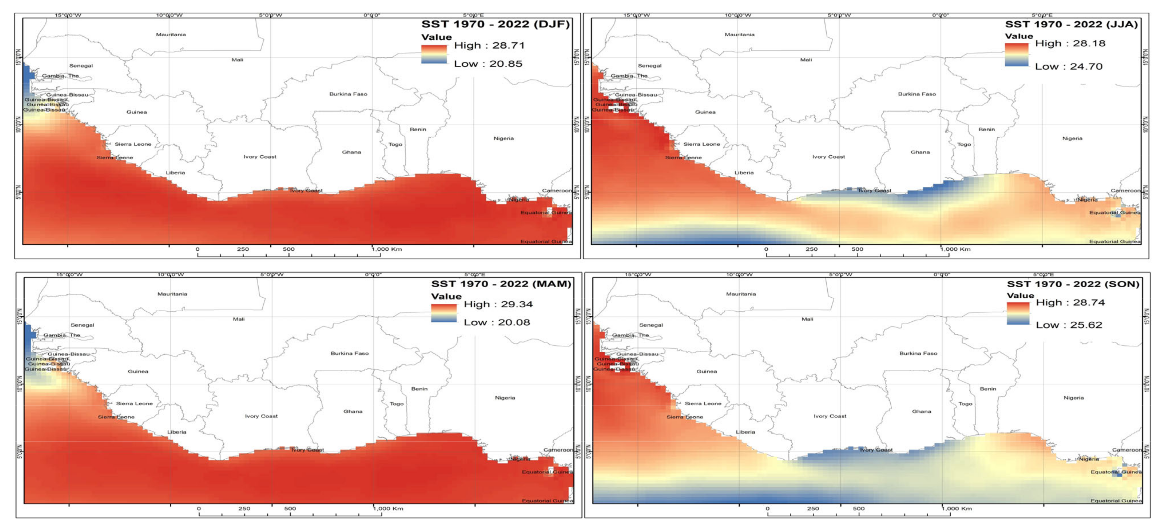
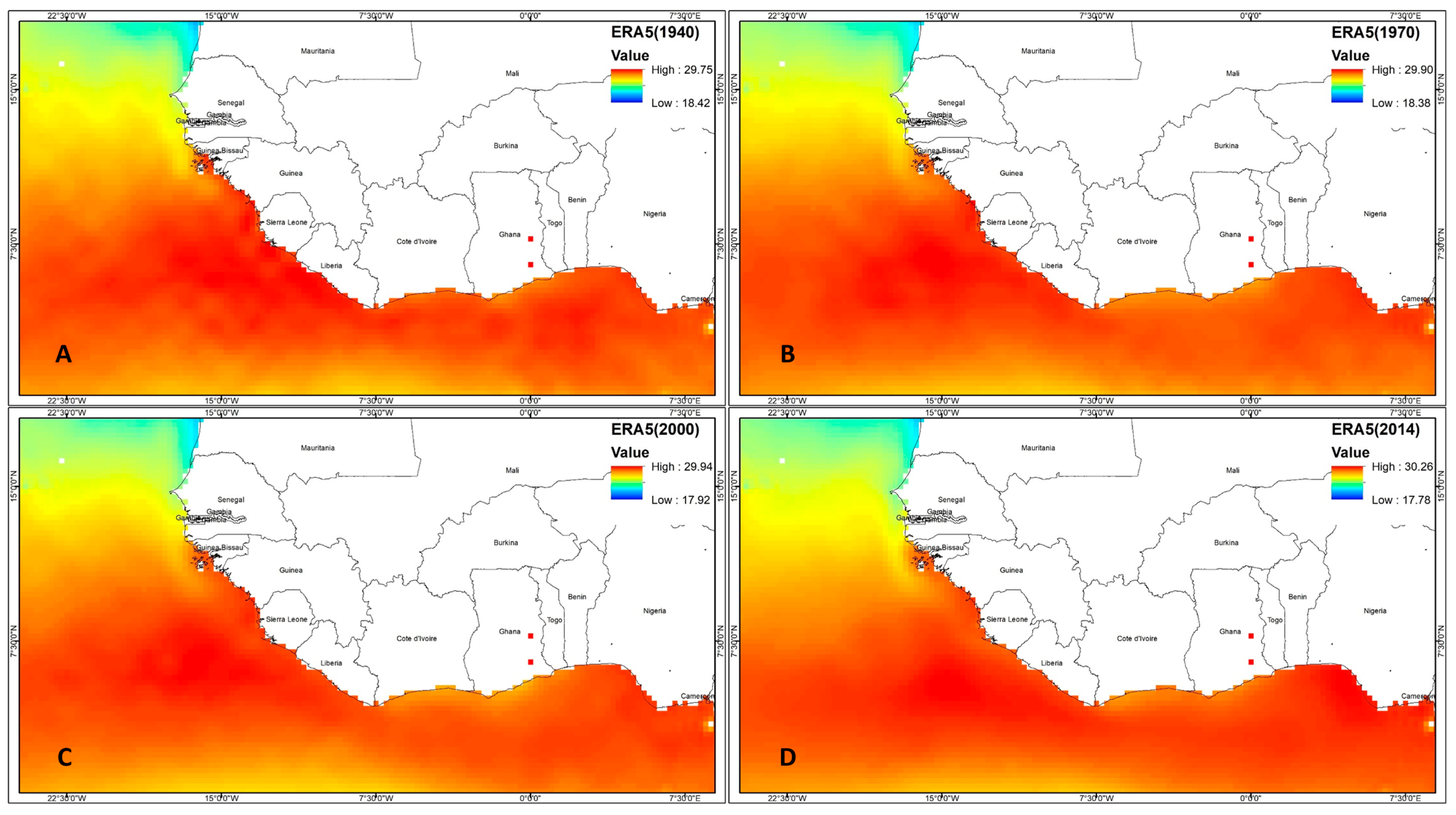
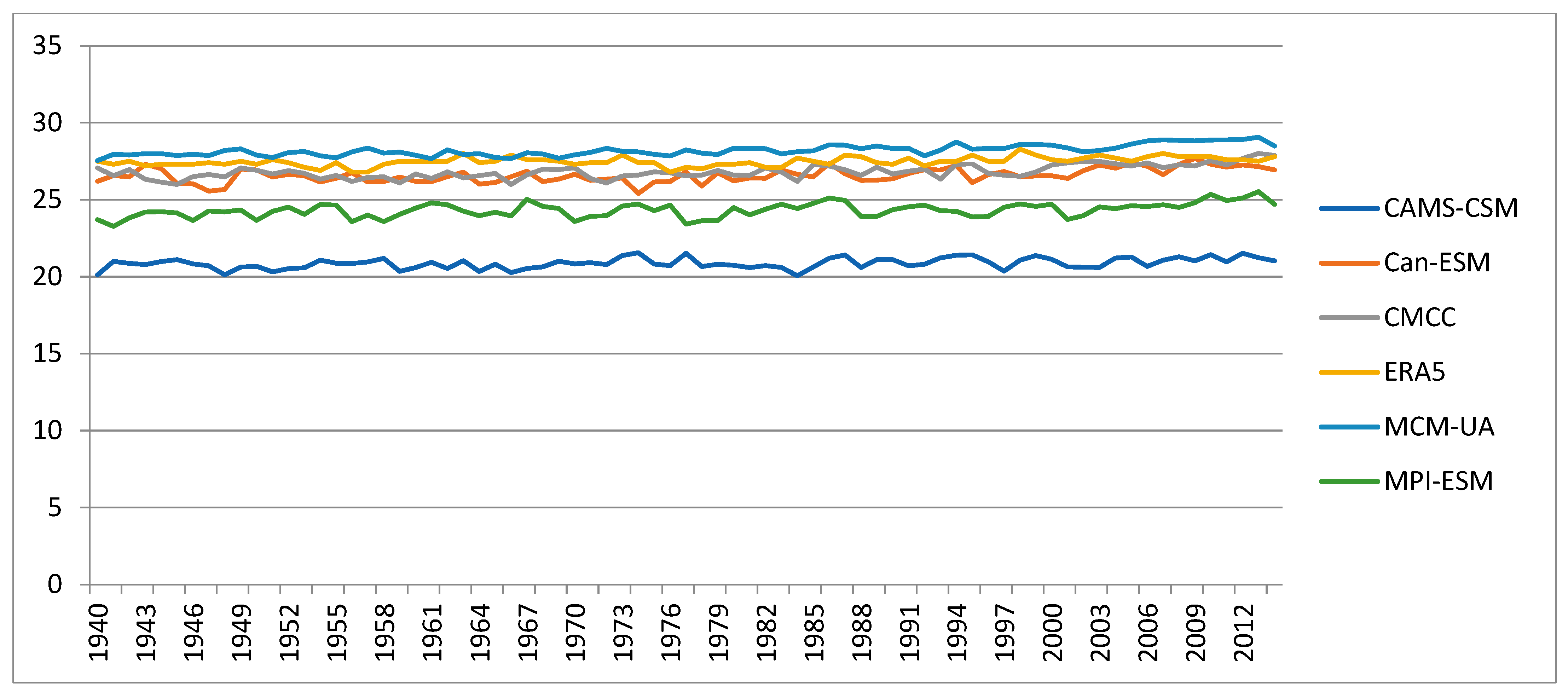
3.1. Historical/Observed SST Climatology
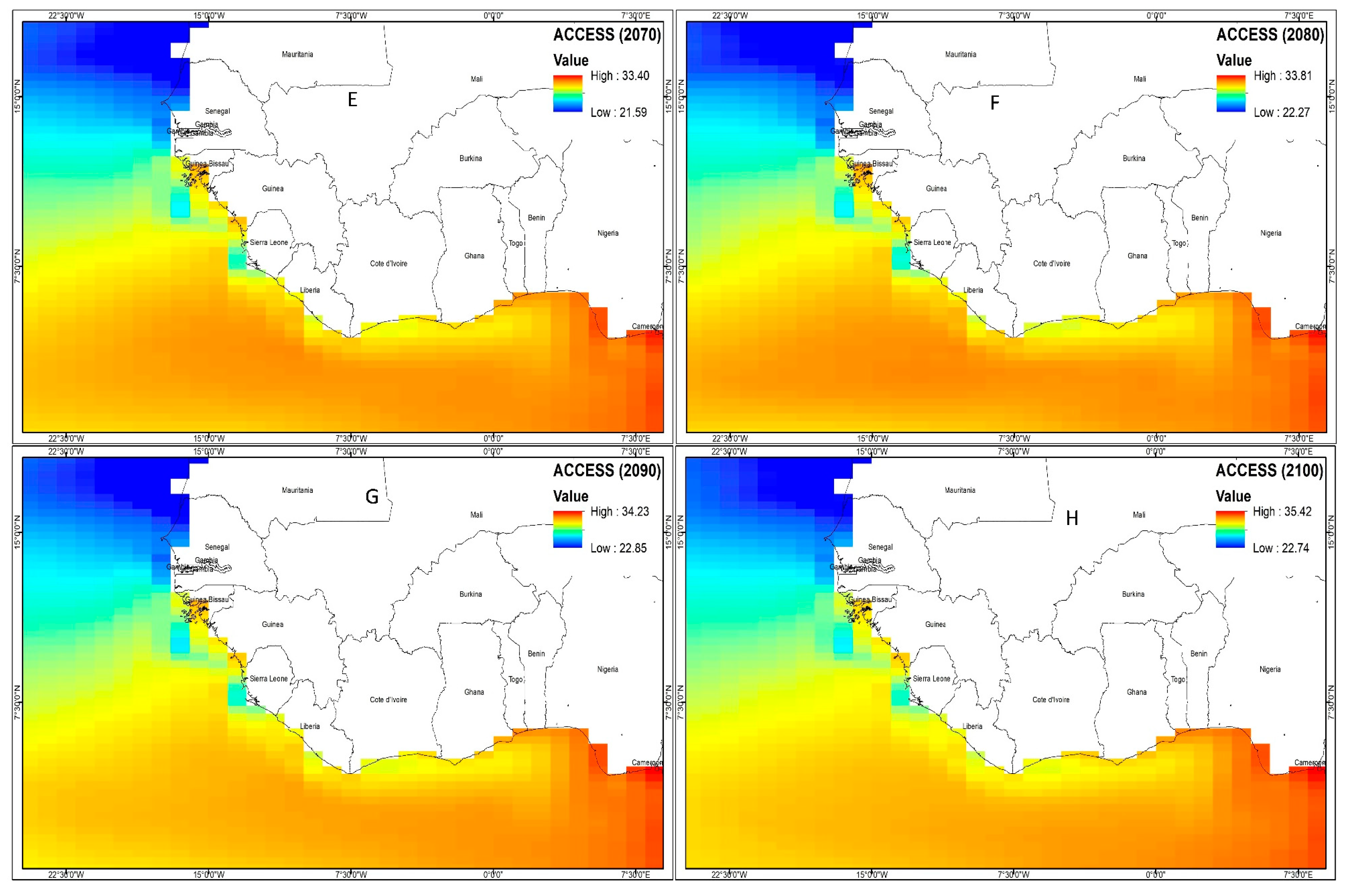
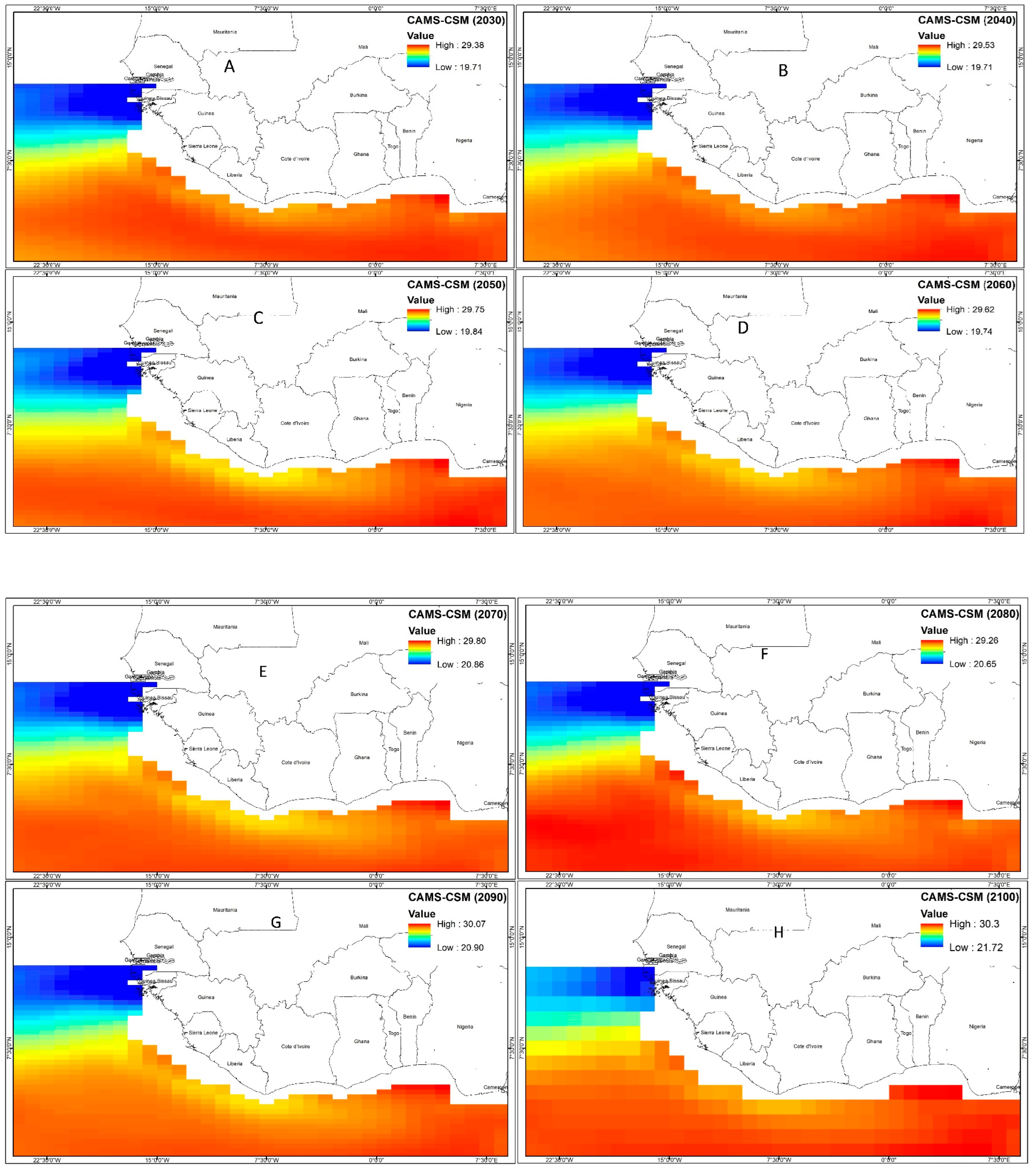
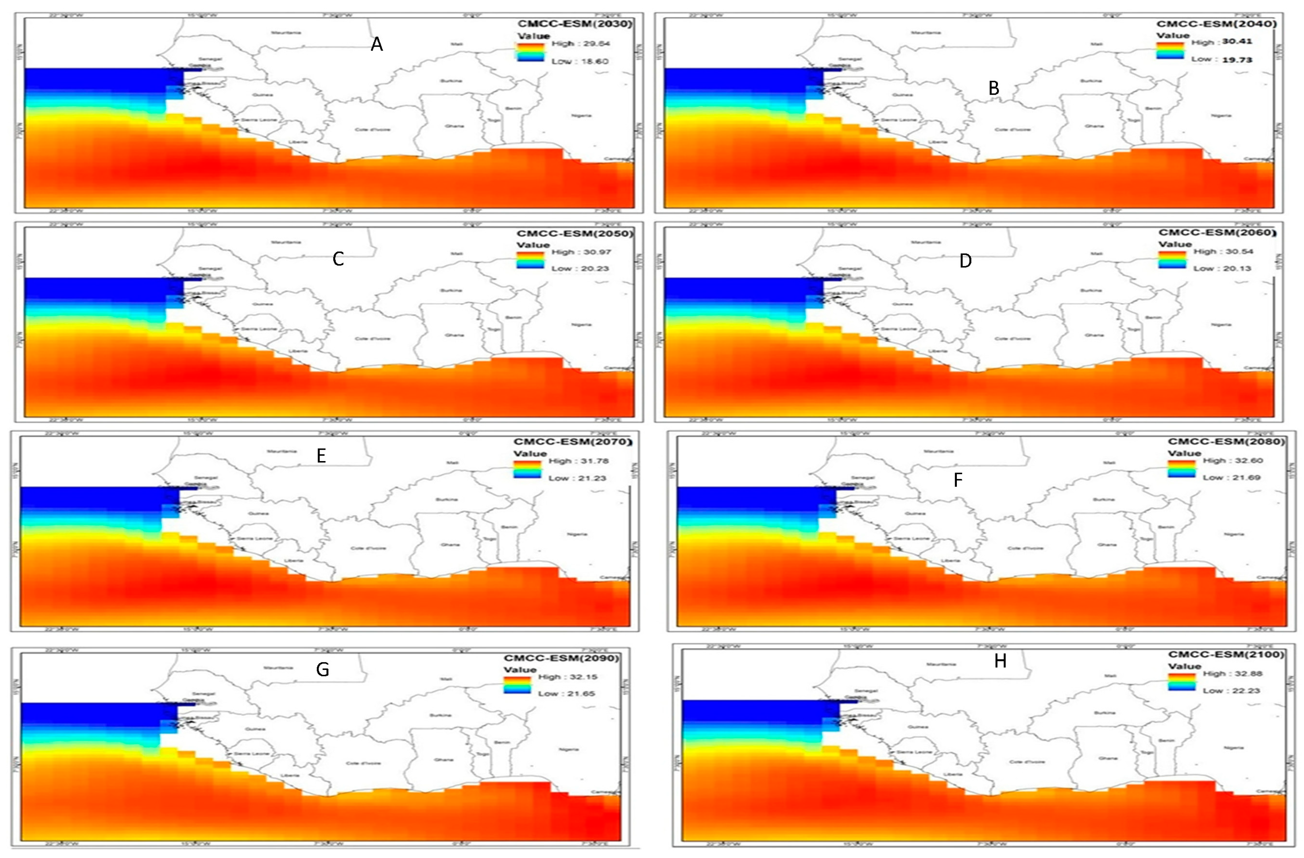
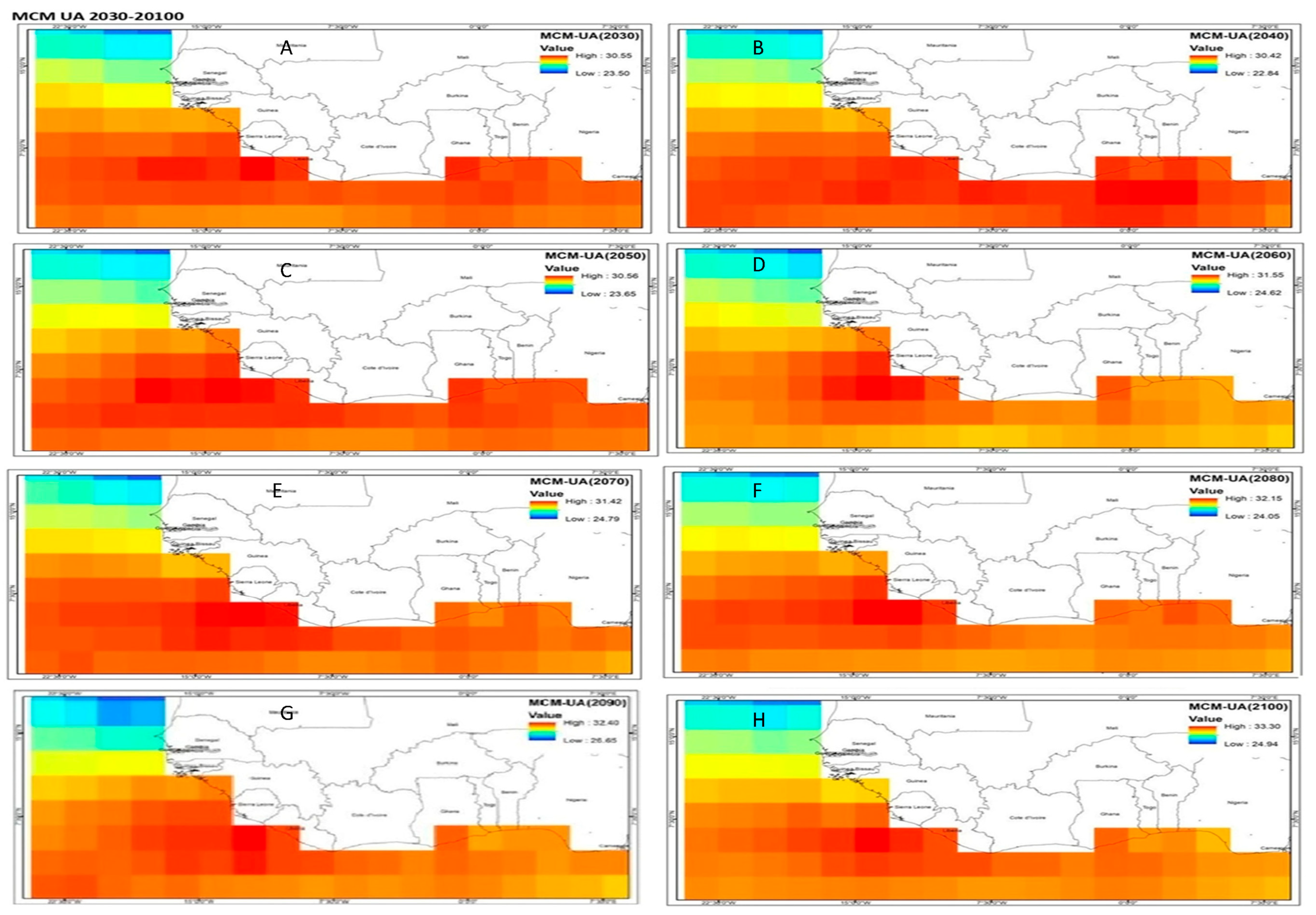
3.2. CMIP6’s Future SST Projection
4. Discussion
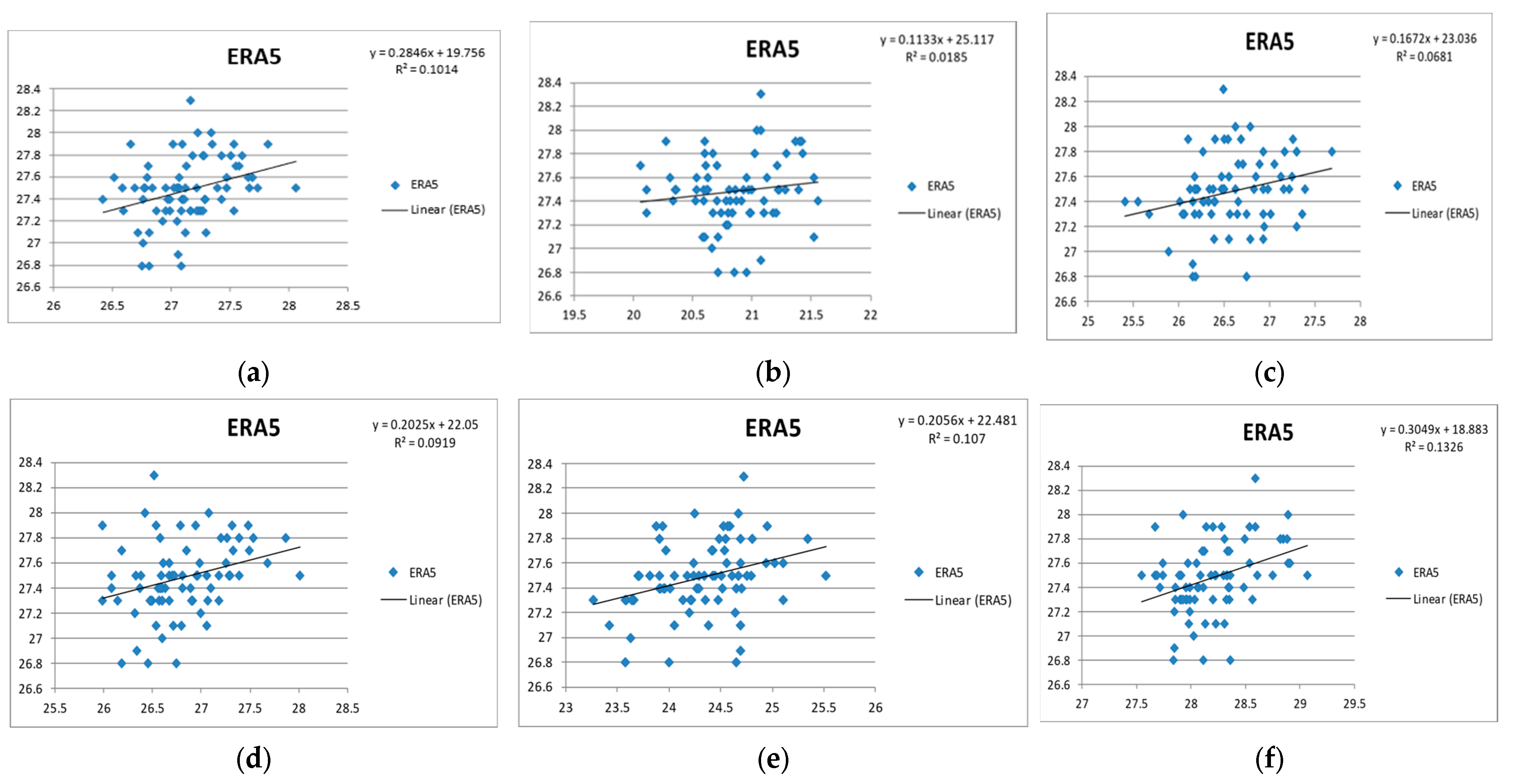
4.1. Statistical Evaluation of the CMIP6 Models’ Performance
Multiple Regression
4.2. Test of Significance
5. Summary and Conclusions
Author Contributions
Funding
Data Availability Statement
Conflicts of Interest
References
- Watson, R.T.; Core Writing Team (Eds.) IPCC: Climate Change 2001: Synthesis Report—A Contribution of Working Groups I, II, and III to the Third Assessment Report of the Intergovernmental Panel on Climate Change; Cambridge University Press: Cambridge, UK; New York, NY, USA, 2001; p. 398. [Google Scholar]
- Wijffels, S.; Roemmich, D.; Monselesan, D.; Church, J.; Gilson, J. Ocean Temperatures Chronicle the Ongoing Warming of Earth. Nat. Clim. Change 2016, 6, 337–342. [Google Scholar] [CrossRef]
- Sung, H.M.; Kim, J.; Lee, J.H.; Shim, S.; Boo, K.O.; Ha, J.C.; Kim, Y.H. Future Changes in the Global and Regional Sea Level Rise and Sea Surface Temperature Based on CMIP6 Models. Atmosphere 2021, 2, 90. [Google Scholar] [CrossRef]
- Roberts, C.D.; Palmer, M.D.; Mcneall, D.; Collins, M. Quantifying the Likelihood of a Continued Hiatus in Global Warming. Nat. Clim. Change 2001, 5, 337. [Google Scholar] [CrossRef]
- Dado, J.M.B.; Takahashi, H.G. Potentail impact of sea surface temperature on rainfall over the western Philippines. Prog. Earth Planet. Sci. 2017, 4, 1–12. [Google Scholar] [CrossRef]
- Lübbecke, J.F.; Belen-Fonseca, B.R.; Richter, I.; Martín-Rey, M.; Losada, T.; Polo, I.; Keenlyside, N.S. Equatorial Atlantic Variability Modes, Mechanisms, and Global Teleconnections. Wiley Interdiscip. Rev. Clim. Change 2018, 9, e527. [Google Scholar] [CrossRef]
- Rowell, D.P. Stimulating SST Teleconnections to Africa: What is the state of the Art? J. Clim. 2013, 26, 5397–5418. [Google Scholar] [CrossRef]
- Palmer, P.I.; Wainwright, C.M.; Dong, B.; Maidment, R.I.; Wheeler, K.G.; Gedney, N.; Hickman, J.E.; Madani, N.; Folwell, S.S.; Abdo, G.; et al. Drivers and Impacts of Eastern African Rainfall Variability. Nat. Rev. Earth Environ. 2023, 4, 254–270. [Google Scholar] [CrossRef]
- Newell, R.E.; Kidson, J.E. African mean wind changes between Sahelian wet and dry periods. J. Climatol. 1984, 4, 27. [Google Scholar] [CrossRef]
- Bah, H. Towards the prediction of Sahelian rainfall from sea surface temperatures in the Gulf of Guinea. Tellus 1987, 39A, 39–48. [Google Scholar] [CrossRef]
- Adeniye, M.O. Modeling the Impact of Changes in Atlantic Sea Surface Temperature on the Climate of West Africa. J. Meteorol. Atmos. Phys. 2017, 129, 187–210. [Google Scholar] [CrossRef]
- World Bank. The Next Generation Africa Climate Business Plan; World Bank: Washington, DC, USA, 2020. [Google Scholar]
- UNFCCC. The State of the Climate: Extreme Events and Major Impacts; UNFCCC: Bonn, Germany, 2021. [Google Scholar]
- Seager, R.; Naik, N.; Vogel, L. Does global warming cause intensified interannual hydroclimate Variability? J. Clim. 2012, 25, 3355–3372. [Google Scholar] [CrossRef]
- IPCC. Climate Change 2007: The Physical Science Basis. Contribution of Working Group I to the Fourth Assessment Report of the Intergovernmental Panel on Climate Change. Cambridge University Press: Cambridge, UK; New York, NY, USA, 2007. [Google Scholar]
- IPCC. Climate Change 2013: The Physical Science Basis. Contribution of Working Group I to the Fifth Assessment Report of the Intergovernmental Panel on Climate Change. Stocker, T.F., Qin, D., Plattner, G.-K., Tignor, M., Allen, S.K., Boschung, J., Nauels, A., Xia, Y., Bex, V., Midgley, P.M., Eds.; Cambridge University Press: Cambridge, UK; New York, NY, USA, 2013; p. 1535. [Google Scholar]
- Burls, N.J.; Reason, C.J.C.; Penven, P.; Philander, S.G. Energetics of the Tropical Atlantic zonal mode. J. Clim. 2012, 25, 7442–7466. [Google Scholar] [CrossRef]
- Breugem, W.P.; Hazeleger, W.; Haarsma, R.J. Multimodal Study of Tropical Atlantic Variability and Change. Geophys. Res. Lett. 2006, 33, L23706. [Google Scholar] [CrossRef]
- Ahmed, K.; Shahid, S.; Sachindra, D.A.; Nawaz, N.; Chung, E.S. Fidelity Assessment of General Circulation Model Simulated Precipitation and Temperature over Pakistan using a Feature Selection Method. J. Hydrol. 2019, 573, 281–298. [Google Scholar] [CrossRef]
- Jose, P.M.; Dwarakish, G.S. Bias Correction and Trend Analysis of Temperature Data by a High-Resolution CMIP6 Model over a Tropical River Basin. Asia-Pac. J. Atmos. Sci. 2022, 58, 97–115. [Google Scholar] [CrossRef]
- Sonali, P.; Kumar, D.N. Review of recent advances in climate change detection and attribution studies: A large-scale hydro climatological perspective. J. Water Clim. Change 2020, 11, 1–29. [Google Scholar] [CrossRef]
- Chokkavarapu, N.; Mandla, V.R. Comparative Study of GCMs, RCMs, Downscaling and Hydrological Models: A review toward future climate change impact estimation. SN Appl. Sci. 2019, 1, 1698. [Google Scholar] [CrossRef]
- Ayugi, B.; Zhihong, J.; Zhu, H.; Ngoma, H.; Babaousmail, H.; Rizwan, K.; Dike, V. Comparison of CMIP6 and CMIP5 models in simulating mean and extreme precipitation over East Africa. Int. J. Climatol. 2021, 41, 6474–6496. [Google Scholar] [CrossRef]
- Liz, Z.; Liu, T.; Huang, Y.; Peng, J.; Ling, Y. Evaluation of the CMIP6 Precipitation Simulations over Global Land. Earth’s Future 2022, 10, 1–21. [Google Scholar]
- Holthuijzen, M.; Beckage, B.; Clemins, P.J.; Higdon, D.; Winter, J.M. Robust bias correction of precipitation extremes using a novel hybrid empirical quantile-mapping method. Theor. Appl. Climatol. 2022, 149, 863–882. [Google Scholar] [CrossRef]
- Ekström, M.; Grose, M.R.; Whetton, P.H. An appraisal of downscaling methods used in climate change research. Clim. Change 2015, 6, 301–319. [Google Scholar] [CrossRef]
- Lafon, T.; Dadson, S.; Buys, G.; Prudhomme, C. Bias correction of daily precipitation simulated by a regional climate model: A comparison of methods. Int. J. Climatol. 2013, 33, 1367–1381. [Google Scholar] [CrossRef]
- Leander, R.; Buishand, T. A Resampling of regional climate model output for the simulation of extreme river flows. J. Hydrol. 2007, 332, 487–496. [Google Scholar] [CrossRef]
- Pierce, D.W.; Cayan, D.R.; Maurer, E.P.; Abatzoglou, J.T.; Hegewisch, K.C. Improved bias correction techniques for hydrological simulations of climate change. J. Hydrometeorol. 2015, 16, 2421–2442. [Google Scholar] [CrossRef]
- Shrestha, M.; Acharya, S.C.; Shrestha, P.K. Bias correction of climate models for hydrological modeling–are simple methods still useful? Meteorol. Appl. 2017, 24, 531–539. [Google Scholar] [CrossRef]
- Hoffmann, H.; Rath, T. Meteorologically consistent bias correction of climate time series for agricultural models. Theor. Appl. Climatol. 2012, 110, 129–141. [Google Scholar] [CrossRef]
- Zia, A.; Bomblies, A.; Schroth, A.W.; Koliba, C.; Isles, P.D.; Tsai, Y.; Mohammed, I.N.; Bucini, G.; Clemins, P.J.; Turnbull, S.; et al. Coupled impacts of climate and land use change across a river–lake continuum: Insights from an integrated assessment model of lake Champlain’s Missisquoi basin, 2000–2040. Environ. Res. Lett. 2016, 11, 114026. [Google Scholar] [CrossRef]
- Trasher, B.; Maurer, E.P.; McKellar, C.; Dufy, P.B. Technical Note: Bias correcting climate model simulated daily temperature extremes with quantile mapping. Hydrol. Earth Syst. Sci. 2012, 16, 3309–3314. [Google Scholar] [CrossRef]
- Maraun, D. Bias correction, quantile mapping, and downscaling: Revisiting the inflation issue. J. Clim. 2010, 26, 2137–2143. [Google Scholar] [CrossRef]
- Giorgi, F.; Gutowski, W.J. Regional Dynamical Downscaling and the CORDEX Initiative. Annu. Rev. Environ. Resour. 2015, 40, 467–490. [Google Scholar] [CrossRef]
- Mearns, L.; Giorgi, F.; Whetton, P.; Pabon, D.; Hulme, M.; Lal, M. Guidelines for Use of Climate Scenarios Developed from Regional Climate Model Experiments; Data Distribution Centre of the Intergovernmental Panel on Climate Change: Geneva, Switzerland, 2003; pp. 1–38. [Google Scholar]
- Feser, F.; Rockel, B.; von Storch, H.; Winterfeldt, J.; Zahn, M. Regional climate models add value to global model data: A review and selected examples. Bull. Am. Meteorol. Soc. 2011, 92, 1181–1192. [Google Scholar] [CrossRef]
- Caldwell, P.; Chin, H.N.S.; Bader, D.C.; Bala, G. Evaluation of a WRF dynamical downscaling simulation over California. Clim. Change 2009, 95, 499–521. [Google Scholar] [CrossRef]
- Leung, L.R.; Mearns, L.O.; Giorgi, F.; Wilby, R.L. Regional climate research: Needs and opportunities. Bull. Am. Meteorol. Soc. 2003, 84, 89–95. [Google Scholar]
- Mearns, L.O.; Sain, S.; Leung, L.R.; Bukovsky, M.S.; McGinnis, S.; Biner, S.; Caya, D.; Arritt, R.W.; Gutowski, W.; Takle, E.; et al. Climate change projections of the North American Regional Climate Change Assessment Program (NARCCAP). Clim. Change 2013, 120, 965–975. [Google Scholar] [CrossRef]
- Hanssen-Bauer, I.; Achberger, C.; Benestad, R.; Chen, D.; Førland, E. Statistical downscaling of climate scenarios over Scandinavia. Clim. Res. 2005, 29, 255–268. [Google Scholar] [CrossRef]
- Gudmundsson, L.; Bremnes, J.B.; Haugen, J.E.; Engen-Skaugen, T. Technical Note: Downscaling RCM precipitation to the station scale using statistical transformations—A comparison of methods. Hydrol. Earth Syst. Sci. 2012, 16, 3383–3390. [Google Scholar] [CrossRef]
- Mudbhatkal, A.; Mahesha, A. Bias correction methods for hydrologic impact studies over India’s Western Ghat basins. J. Hydrol. Eng. 2018, 23, 05017030. [Google Scholar] [CrossRef]
- Smitha, P.S.; Narasimhan, B.; Sudheer, K.P.; Annamalai, H. An improved bias correction method of daily rainfall data using a sliding window technique for climate change impact assessment. J. Hydrol. 2018, 556, 100–118. [Google Scholar] [CrossRef]
- Mendez, M.; Maathuis, B.; Hein-Griggs, D.; Alvarado-Gamboa, L.F. Performance evaluation of bias correction methods for climate change monthly precipitation projections over Costa Rica. Water 2020, 12, 482. [Google Scholar] [CrossRef]
- White, R.H.; Toumi, R. The limitations of bias correcting regional climate model inputs. Geophys. Res. Lett. 2013, 40, 2907–2912. [Google Scholar] [CrossRef]
- Lanzante, J.R.; Dixon, K.W.; Adams-Smith, D.; Nath, M.J.; Whitlock, C.E. Evaluation of some distributional downscaling methods as applied to daily precipitation with an eye towards extremes. Int. J. Climatol. 2021, 41, 3186–3202. [Google Scholar] [CrossRef]
- Christensen, J.H.; Boberg, F.; Christensen, O.B.; Lucas-Picher, P. On the Need for Bias Correction of Regional Climate Change Projections of Temperature and Precipitation. J. Geophys. Res. Lett. 2008, 35, L20709. [Google Scholar] [CrossRef]
- Byun, K.; Hamlet, A.F. An improved empirical quantile mapping procedure for bias-correction of climate change projections. In Proceedings of the An American Geophysical Union, Fall Meeting, San Francisco, CA, USA, 9–13 December 2019. [Google Scholar]
- Heo, J.; Ahn, H.; Shin, J.; Kjeldsen, T.; Jeong, C. Probability Distributions for a Quantile Mapping Technique for a Bias Correction of Precipitation Data: A Case Study to Precipitation Data Under Climate Change. Water 2019, 11, 1475. [Google Scholar] [CrossRef]
- Déqué, M. Frequency of precipitation and temperature extremes over France in an anthropogenic scenario: Model results and statistical correction according to observed values. Glob. Planet Change 2007, 57, 16–26. [Google Scholar] [CrossRef]
- Shabalova, M.V.; van Deursen, W.P.; Buishand, T.A. Assessing future discharge of the river Rhine using regional climate model integrations and a hydrological model. Clim. Res. 2003, 23, 233–246. [Google Scholar] [CrossRef]
- Teutschbein, C.; Seibert, J. Bias correction of regional climate model simulations for hydrological climate-change impact studies: Review and evaluation of different methods. J. Hydrol. 2012, 456, 12–29. [Google Scholar] [CrossRef]
- Ezéchiel, O.; Eric, A.A.; Josué, Z.E.; Eliézer, B.I.; Amédée, C. Comparative study of seven bias correction methods applied to three Regional Climate Models in Mekrou catchment (Benin, West Africa). Int. J. Curr. Eng. Technol. 2016, 6, 1831–1840. [Google Scholar]
- Amengual, A.; Homar, V.; Romero, R.; Alonso, S.; Ramis, C. A statistical adjustment of regional climate: Application to Platja de Palma. Spain J. Clim. 2012, 25, 939–957. [Google Scholar] [CrossRef]
- Gutjahr, O.; Heinemann, G. Comparing precipitation bias correction methods for high-resolution regional climate simulations using COSMO-CLM: Effects on extreme values and climate change signal. Theor. Appl. Climatol. 2013, 114, 511–529. [Google Scholar] [CrossRef]
- Volosciuk, C.; Maraun, D.; Vrac, M.; Widmann, M. A combined statistical bias correction and stochastic downscaling method for precipitation. Hydrol. Earth Syst. Sci. 2017, 21, 1693–1719. [Google Scholar] [CrossRef]
- Li, H.; Sheffield, J.; Wood, E.F. Bias correction of monthly precipitation and temperature fields from intergovernmental panel on climate change AR4 models using equidistant quantile matching. J. Geophys. Res. Atmos. 2010, 115, 1–20. [Google Scholar] [CrossRef]
- Cannon, A.J.; Sobie, S.R.; Murdock, T.Q. Bias correction of GCM precipitation by quantile mapping: How well do methods preserve changes in quantiles and extremes? J. Clim. 2015, 28, 6938–6959. [Google Scholar] [CrossRef]
- Sahoo, S.; Dey, S.; Dhar, A.; Debsakar, A.; Predham, B. On projected hydrological scenarios under the influence of bias-corrected climatic variables and LULC. Ecol. Indic. 2019, 106, 105440. [Google Scholar] [CrossRef]
- Eyring, V.; Bony, S.; Meehl, G.A.; Senior, C.A.; Stevens, B.; Stouffer, R.J.; Taylor, K.E. Overview of the Coupled Model Intercomparison Project Phase 6 (CMIP6) experimental design and organization. Geosci. Model Dev. 2016, 9, 1937–1958. [Google Scholar] [CrossRef]
- Gidden, M.J.; Riahi, K.; Smith, S.J.; Fujimori, S.; Luderer, G.; Kriegler, E.; Van Vuuren, D.P.; Van Den Berg, M.; Feng, L.; Klein, D.; et al. Global emissions pathways under different socioeconomic scenarios for use in CMIP6: A dataset of harmonized emissions trajectories through the end of the century. Geosci. Model Dev. 2019, 12, 1443–1475. [Google Scholar] [CrossRef]
- Odekunle, T.O.; Eludoyin, A.O. Sea surface temperature pattern and its implication on rainfall variability over the Gulf of Guinea. Int. J. Climatol. 2008, 28, 1507–1517. [Google Scholar] [CrossRef]
- Ojo, O. The Climates of West Africa; Heinemann: London, UK, 1977; p. 219. [Google Scholar]
- Iloeje, N.P. A New Geography of Nigeria; Longman: London, UK, 1981; p. 259. [Google Scholar]
- Raper, S.C.B.; Cubasch, U. Emulation of the Results from a Coupled General Circulation Model using a Simple Climate Model. Geophys. Res. Lett. 1996, 23, 1107–1110. [Google Scholar] [CrossRef]
- Siongco, A.C.; Hohenegger, C.; Stevens, B. The Atlantic ITCZ bias in CMIP5 models. Clim. Dyn. 2015, 45, 5–6. [Google Scholar] [CrossRef]
- Steinig, S.; Harlaß, J.; Park, W.; Latif, M. Sahel rainfall strength and onset improvements due to more realistic Atlantic cold tongue development in a climate model. Sci. Rep. 2018, 8, 2569. [Google Scholar] [CrossRef] [PubMed]
- Dunning, C.M.; Allan, R.P.; Black, E. Identification of deficiencies in seasonal rainfall simulated by CMIP5 climate models. Environ. Res. Lett. 2017, 12, 1748–9326. [Google Scholar] [CrossRef]
- Brown, J.N.; Langlais, C.; Gupta, A.S. Projected Sea Surface Temperature Changes in the Equatorial Pacific Relative to the Warm Pool Edge. Elsevier J. Sea Res. 2015, 11, 47–58. [Google Scholar] [CrossRef]
- Bhatt, B.C.; Sobolowski, S.; Higuchi, A. Simulation of Diurnal Rainfall variability over the maritime continent with high-resolution regional climate model. J. Jpn. Meteorol. Soc. Jpn. 2016, 94A, 89–103. [Google Scholar] [CrossRef]
- Cai, T.T.; Guo, Z.; Ma, R. Statistical Inference for High-Dimensional Generalized Linear Models with Binary Outcomes. J. Am. Statitsical Assoc. 2021, 118, 1319–1332. [Google Scholar] [CrossRef] [PubMed]
- Rhymee, H.; Shams, S.; Ratnayake, U.; Rahman, E.K.A. Comparing Statistical Downscaling and Arithmetic Mean in Simulating CMIP6 Multi-Model Ensemble over Brunei. Hydrology 2022, 9, 161. [Google Scholar] [CrossRef]


| Data | Type | Temporal | Historical | Future |
|---|---|---|---|---|
| ERA5 | Observed | Monthly | 1940–2014 | --- |
| ACCESS-CM2 (Australia) | Model | Monthly | 1940–2014 | 2030–2100 |
| CAMS-CSM1-0 (China) | Model | Monthly | 1940–2014 | 2030–2100 |
| CanESM5-CanOE (Canada) | Model | Monthly | 1940–2014 | 2030–2100 |
| CMCC-ESM2 (Italy) | Model | Monthly | 1940–2014 | 2030–2100 |
| HadGEM3-GC31-LL (UK) | Model | Monthly | 1940–2014 | 2030–2100 |
| EC-Earth3-CC (Europe) | Model | Monthly | 1940–2014 | 2030–2100 |
| MCM-UA-1-0 (USA) | Model | Monthly | 1940–2014 | 2030–2100 |
| MPI-ESM1-2-LR (Germany) | Model | Monthly | 1940–2014 | 2030–2100 |
| Climate Modeling Centers | CMIPs | Spatial Resolution | Number of Simulations | Future Scenarios | ||
|---|---|---|---|---|---|---|
| Historical Period | Future Periods | |||||
| Can ESM | CanESM2 | 1.0° × 1.0° | 1940–2022 | 2014–2100 | 8.5 | RCPs 4.5 and 8.5 |
| CanESM5 | 1.0° × 1.0° | 1940–2022 | 2014–2100 | 85 | SSPs 2–4.5 and 5–8.5 | |
| CMCC-ESM | CMCC-ESM | 1.0° × 1.0° | 1940–2022 | 2014–2100 | 8.5 | RCPs 4.5 and 8.5 |
| CMCC-ESM | 1.0° × 1.0° | 1940–2022 | 2014–2100 | 8.5 | SSPs 2–4.5 and 5–8.5 | |
| ACCESS | ACCESS | 1.0° × 1.0° | 1940–2022 | 2014–2100 | 85 | RCPs 4.5 and 8.5 |
| ACCESS | 1.0° × 1.0° | 1940–2022 | 2014–2100 | 8.5 | SSPs 2–4.5 and 5–8.5 | |
| EC-Earth3 | EC-Earth3 | 1.4° × 1.5° | 1940–2022 | 2014–2100 | 8.5 | RCPs 4.5 and 8.5 |
| EC-Earth3 | 1.4° × 1.4° | 1940–2022 | 2014–2100 | 8.5 | SSPs 2–4.5 and 5–8.5 | |
| MPI | MPI-ESM-LR | 1.0° × 1.0° | 1940–2022 | 2014–2100 | 8.5 | RCPs 4.5 and 8.5 |
| MPI-ESM1-2-LR | 1.0° × 1.0° | 1940–2022 | 2014–2100 | 8.5 | SSPs 2–4.5 and 5–8.5 | |
| MCM-UA | MCM-UA | 2.0° × 2.0° | 1940–2022 | 2014–2100 | 8.5 | RCPs 4.5 and 8.5 |
| MCM-UA | 2.0° × 2.0° | 1940–2022 | 2014–2100 | 8.5 | SSPs 2–4.5 and 5–8.5 | |
| ERA5 | ACCESS | CAMS | CanESM | CMCC | MCM | ||
|---|---|---|---|---|---|---|---|
| Pearson Correlation | ERA5 | 1.000 | 0.318 | 0.136 | 0.261 | 0.303 | 0.364 |
| ACCESS | 0.318 | 1.000 | 0.378 | 0.318 | 0.522 | 0.497 | |
| CAMS | 0.136 | 0.378 | 1.000 | 0.230 | 0.274 | 0.466 | |
| CanESM | 0.261 | 0.318 | 0.230 | 1.000 | 0.463 | 0.525 | |
| CMCC | 0.303 | 0.522 | 0.274 | 0.463 | 1.000 | 0.559 | |
| MCM | 0.364 | 0.497 | 0.466 | 0.525 | 0.559 | 1.000 | |
| MPI | 0.327 | 0.177 | 0.241 | 0.349 | 0.399 | 0.460 | |
| Sig. (1-tailed) | ERA5 | 0.003 | 0.122 | 0.012 | 0.004 | 0.001 | |
| ACCESS | 0.003 | 0.000 | 0.003 | 0.000 | 0.000 | ||
| CAMS | 0.122 | 0.000 | 0.024 | 0.009 | 0.000 | ||
| CanESM | 0.012 | 0.003 | 0.024 | 0.000 | 0.000 | ||
| CMCC | 0.004 | 0.000 | 0.009 | 0.000 | 0.000 | ||
| MCM | 0.001 | 0.000 | 0.000 | 0.000 | 0.000 | ||
| MPI | 0.002 | 0.065 | 0.018 | 0.001 | 0.000 | 0.000 | |
| N | ERA5 | 75 | 75 | 75 | 75 | 75 | 75 |
| ACCESS | 75 | 75 | 75 | 75 | 75 | 75 | |
| CAMS | 75 | 75 | 75 | 75 | 75 | 75 | |
| CanESM | 75 | 75 | 75 | 75 | 75 | 75 | |
| CMCC | 75 | 75 | 75 | 75 | 75 | 75 | |
| MCM | 75 | 75 | 75 | 75 | 75 | 75 | |
| MPI | 75 | 75 | 75 | 75 | 75 | 75 | |
| Model | Sum of Squares | df | Mean Square | F | Sig. | |
|---|---|---|---|---|---|---|
| 1 | Regression | 0.837 | 1 | 0.837 | 11.161 | 0.001 b |
| Residual | 5.477 | 73 | 0.075 | |||
| Total | 6.314 | 74 | ||||
| Model | Unstandardized Coefficients | Standardized Coefficients | t | Sig. | ||
|---|---|---|---|---|---|---|
| B | Std. Error | Beta | ||||
| 1 | (Constant) | 18.883 | 2.574 | 7.336 | 0.000 | |
| MCM | 0.305 | 0.091 | 0.364 | 3.341 | 0.001 | |
| Collinearity Diagnostics | |||||||
|---|---|---|---|---|---|---|---|
| Model | Dimension | Eigenvalue | Condition Index | Variance Proportions | |||
| (Constant) | ACCESS | MCMUA | MPIESM | ||||
| 1 | 1 | 1.999 | 1.000 | 0.00 | 0.00 | ||
| 2 | 0.001 | 43.820 | 1.00 | 1.00 | |||
| 2 | 1 | 2.999 | 1.000 | 0.00 | 0.00 | 0.00 | |
| 2 | 0.001 | 52.817 | 0.30 | 0.07 | 0.00 | ||
| 3 | 5.885 × 10⁻⁵ | 225.739 | 0.70 | 0.93 | 1.00 | ||
| 3 | 1 | 3.999 | 1.000 | 0.00 | 0.00 | 0.00 | 0.00 |
| 2 | 0.001 | 60.981 | 0.22 | 0.06 | 0.00 | 0.00 | |
| 3 | 0.000 | 175.706 | 0.31 | 0.13 | 0.04 | 0.99 | |
| 4 | 5.869 × 10⁻⁵ | 261.029 | 0.46 | 0.81 | 0.96 | 0.01 | |
| 4 | 1 | 4.999 | 1.000 | 0.00 | 0.00 | 0.00 | 0.00 |
| 2 | 0.001 | 66.901 | 0.20 | 0.04 | 0.00 | 0.00 | |
| 3 | 0.000 | 188.768 | 0.19 | 0.02 | 0.01 | 0.95 | |
| 4 | 6.915 × 10⁻⁵ | 268.854 | 0.06 | 0.14 | 0.33 | 0.05 | |
| 5 | 5.783 × 10⁻⁵ | 294.013 | 0.54 | 0.81 | 0.66 | 0.00 | |
Disclaimer/Publisher’s Note: The statements, opinions and data contained in all publications are solely those of the individual author(s) and contributor(s) and not of MDPI and/or the editor(s). MDPI and/or the editor(s) disclaim responsibility for any injury to people or property resulting from any ideas, methods, instructions or products referred to in the content. |
© 2024 by the authors. Licensee MDPI, Basel, Switzerland. This article is an open access article distributed under the terms and conditions of the Creative Commons Attribution (CC BY) license (https://creativecommons.org/licenses/by/4.0/).
Share and Cite
Ideki, O.; Lupo, A.R. Evaluation of Bias-Corrected GCM CMIP6 Simulation of Sea Surface Temperature over the Gulf of Guinea. Climate 2024, 12, 19. https://doi.org/10.3390/cli12020019
Ideki O, Lupo AR. Evaluation of Bias-Corrected GCM CMIP6 Simulation of Sea Surface Temperature over the Gulf of Guinea. Climate. 2024; 12(2):19. https://doi.org/10.3390/cli12020019
Chicago/Turabian StyleIdeki, Oye, and Anthony R. Lupo. 2024. "Evaluation of Bias-Corrected GCM CMIP6 Simulation of Sea Surface Temperature over the Gulf of Guinea" Climate 12, no. 2: 19. https://doi.org/10.3390/cli12020019
APA StyleIdeki, O., & Lupo, A. R. (2024). Evaluation of Bias-Corrected GCM CMIP6 Simulation of Sea Surface Temperature over the Gulf of Guinea. Climate, 12(2), 19. https://doi.org/10.3390/cli12020019