Article

Machine Learning Identification of Attributes and Predictors for a Flash Drought in Eastern Australia

1
School of Mathematical and Physical Sciences, University of Technology Sydney, Sydney, NSW 2007, Australia
2
The Climate Risk Group, Newcastle, NSW 2300, Australia
*
Author to whom correspondence should be addressed.
Climate 2024, 12(4), 49; https://doi.org/10.3390/cli12040049
Submission received: 14 March 2024 / Revised: 31 March 2024 / Accepted: 3 April 2024 / Published: 8 April 2024
(This article belongs to the Special Issue Addressing Climate Change with Artificial Intelligence Methods)

Abstract

:
Flash droughts (FDs) are natural disasters that strike suddenly and intensify quickly. They occur almost anywhere, anytime of the year, and can have severe socio-economic, health and environmental impacts. This study focuses on a recent FD that began in the cool season of the Upper Hunter region of Eastern Australia, an important energy and agricultural local and global exporter that is both flood- and drought-prone. Here, the authors investigate the FD that started abruptly in May 2023 and extended to October 2023. The FD followed floods in November 2021 and much above-average May–October 2022 rainfall. Eight machine learning (ML) regression techniques were applied to the 60 May–October periods from 1963–2022, using a rolling windows attribution search from 45 possible climate drivers, both individually and in combination. The six most prominent climate drivers, and likely predictors, provide an understanding of the major contributors to the FD. Next, the 1963–2022 data were divided into two shorter timespans, 1963–1992 and 1993–2022, generally accepted as representing the early and accelerated global warming periods, respectively. The key attributes were markedly different for the two timespans. These differences are readily explained by the impacts of global warming on hemispheric and synoptic-scale atmospheric circulations.

1. Introduction

A flash drought (FD) occurred in Eastern Australia between May and October 2023 after record rainfall in the same period in 2022. At the end of April 2023, most of the state of New South Wales in southeast Australia showed no indicators of an impending agricultural drought. As defined by the New South Wales Department of Primary Industry [1], these factors include decreased rainfall, increased heat and reduced plant growth (Figure 1a). The USA National Oceanic and Atmospheric Administration (NOAA) defines a FD as “the rapid onset or intensification of drought that develops from a period of low precipitation accompanied by higher-than-average temperatures.” The higher temperatures increase both the evaporation of water from the soil and transpiration from plants (evapotranspiration), further lowering soil moisture, which decreases rapidly as drought conditions continue. FDs can occur at any time of year in Australia [2]. Although FDs mostly occur in summer and autumn in Australia, they can also occur in winter in southeast and southwest Australia [3]. In May 2023, there was an abrupt decrease in rainfall over southeast Australia, which continued until November in the Upper Hunter region (Figure 1b). The consensus is that the primary contribution to FD is precipitation deficit, while evapotranspiration intensifies it [2,4,5,6]. The focus region of this study is the Upper Hunter region of Eastern Australia, which experienced a FD in the period May to October 2023, as defined by the New South Wales state Department of Primary Industry (NSW DPI; Figure 1b). In marked contrast, from May to October 2022, the Upper Hunter region, including the towns of Aberdeen, Muswellbrook, Scone, Rouchel Brook and Bunnan, experienced Decile 10 rainfall (very much above average) (Figure 1c), followed by Decile 1 (very much below average) from May to October 2023 (Figure 1d). Concurrently, from May to October 2023, mean maximum temperatures were the highest on record (Figure 1e), which enhanced the onset of drought by increasing evapotranspiration levels. FDs are often disastrous for the local economy of any region. FDs pose a significant risk to agricultural productivity [7,8], especially in cropping and grassland areas [5], which comprise most of the Upper Hunter region.
The potential for applying current and future applications of Machine Learning (ML) techniques to FD is discussed in the review by Tyagi et al. [5]. A key feature of ML is the ability to deal with multi-source data, non-linearity, multicollinearity and non-stationarity by identifying regional attributes [5]. A recent study by the co-authors was the detection of attributes for the increasingly higher summer maximum temperatures in western Sydney compared with coastal Sydney [9].
Here, the authors concentrate on rainfall variability and use ML techniques on the FD data from May to October 2023 in the Upper Hunter region to identify the most important climate drivers (attributes) that can be employed as predictors of rapid changes in rainfall associated with the FD. This FD varies in characteristics from a typical FD in the literature review of Tyagi et al. [5]. It was generated by a severe precipitation deficiency early in the cool season (May to September) and enhanced by record warm temperatures within the same cool season period (May to October). This differs from the warm season noted as the most common time for FD occurrence by Tyagi et al. [5]. Furthermore, climate drivers such as ENSO and IOD were not applicable at the start of the rapid decline in rainfall in May. However, ENSO did become a factor as the FD developed during the cool season, when lower rainfall months can first appear in an El Niño phase of ENSO. Following the Materials and Methods section, the Results section starts with a rainfall time series for the Upper Hunter accompanied by statistical significance testing of the May to October rainfall mean and variance of the pre- and accelerated global warming periods in the data. Next, the dominant attributes of the FD are assessed by ML techniques from a broad range of potential attributes. The Discussion section draws implications on the validity and limitations of the ML techniques used in this study, with further explanations drawing on observed tropospheric circulation changes.

2. Materials and Methods

2.1. Data Sources

May to October total monthly rainfall data from 1963–2023, representing the Upper Hunter region of the state of New South Wales (NSW) in Eastern Australia, were obtained from the Australian Bureau of Meteorology rainfall for Bunnan, Aberdeen, Scone, Muswellbrook and Rouchel Brook, as indicated in Figure 1. Missing Aberdeen values were substituted by Muswellbrook, the closest station. Missing values for Scone were substituted by values from the closest station, Jerrys Plains, whereas Rouchel Brook and Bunnan had complete data. All precipitation data are available online at: http://www.bom.gov.au/climate/data/ (accessed on 7 March 2024).
To detect statistically significant differences in the dataset, the authors perform permutation testing. To assess the impacts of accelerated GW on May to October Upper Hunter precipitation, the dataset was split into two 30-year periods, 1963–1992 and 1993–2022, with the second period aligning with accelerated global warming (GW) from the 1990s [10,11,12,13] and accelerated GW impacts in southeast Australia [9,14]. Hence, the data for the entire period are non-stationary. Permutation testing of data (without replacement) between two different time periods does not require the data time series to represent a stationary distribution or rely on other underlying assumptions of a parametric distribution [15,16]. Permutation testing was performed on differences in the means and the variances between the two periods.
The climate drivers listed by acronym are identified in Table 1 below. Tasman Sea sea-surface temperature anomalies (TSSSTA) were obtained from the Australian Bureau of Meteorology online climate data archives: http://www.bom.gov.au/cgi-bin/climate/change/timeseries.cgi?graph=sst&area=tas&season=05&ave_yr=0&ave_period=6190 (accessed on 7 March 2024) and all other monthly/seasonal values are available online from the NOAA/PSL websites: https://psl.noaa.gov/gcos_wgsp/Timeseries.index.html or https://psl.noaa.gov/climateindices/index.html (accessed on 7 March 2024). These oceanic and atmospheric climate drivers are known to have an influence on the Eastern Australian climate and were used in several previous studies as possible attributes [9,17,18,19].

2.2. Methods

Both linear and non-linear ML techniques were used to identify the attributes (for possible predictors) that explain trends found in the May–October precipitation time series for the Upper Hunter region. The predictor variables were considered individually as climate drivers in addition to two-way interactions (scalar multiplication between climate drivers), which are intended to account for the compound influence of drivers. Greater than two-way interactions were not considered because they are time-prohibitive. The linear method used was linear regression with both forward and backward selection. Two non-linear methods, Support Vector Regression (SVR) and Random Forests (RF), were employed, both with forward and backward selection, in addition to using both radial basis (RBF) and polynomials (Poly) as the kernel function. Therefore, a total of eight different methods were considered. These methods are explained in more detail in previous studies [9,17,19]. Each of the eight methods used a training/testing split of 10 for rolling windows, where the training window moves forward by one year for each fitted model. Hence, the first training/testing period is 1963–1972/1973–1982, followed by 1964–1973/1974–1983, and ending in 2003–2012/2013–2022. This results in 41 combined training/testing windows to cover the full 60 years in the 1963–2022 non-stationary precipitation time series. A schematic figure of the training/test method is shown schematically in Figure 2.

3. Results

3.1. Exploratory Data Analysis

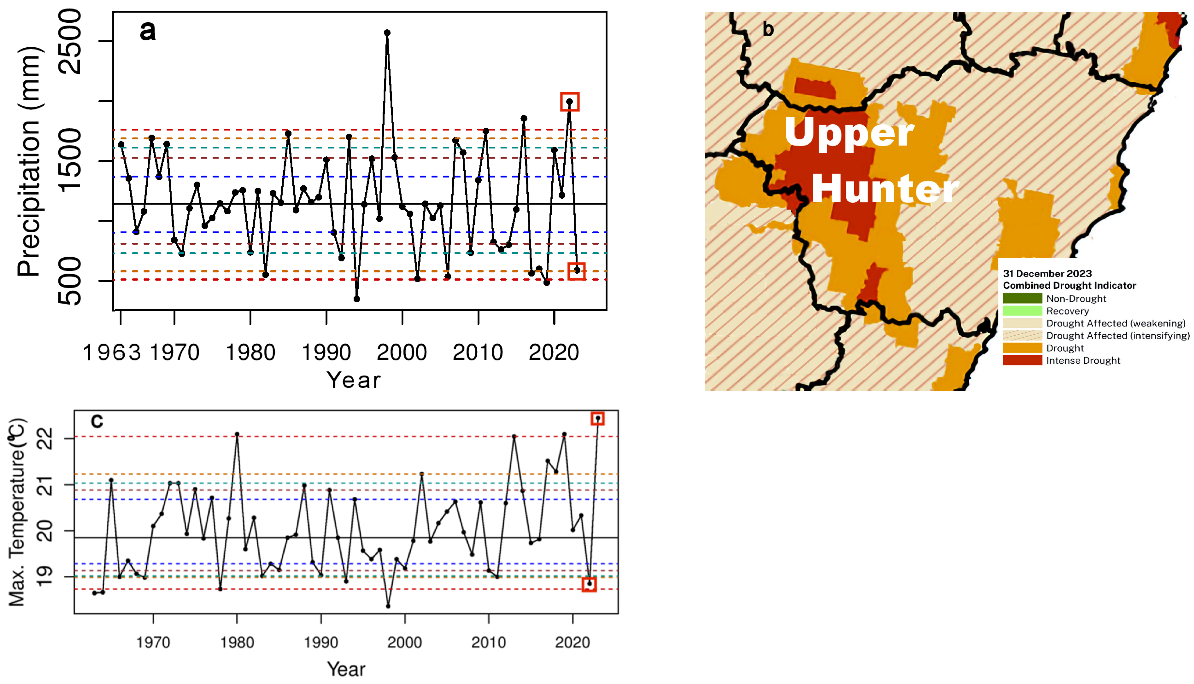
3.1.1. Precipitation Time Series
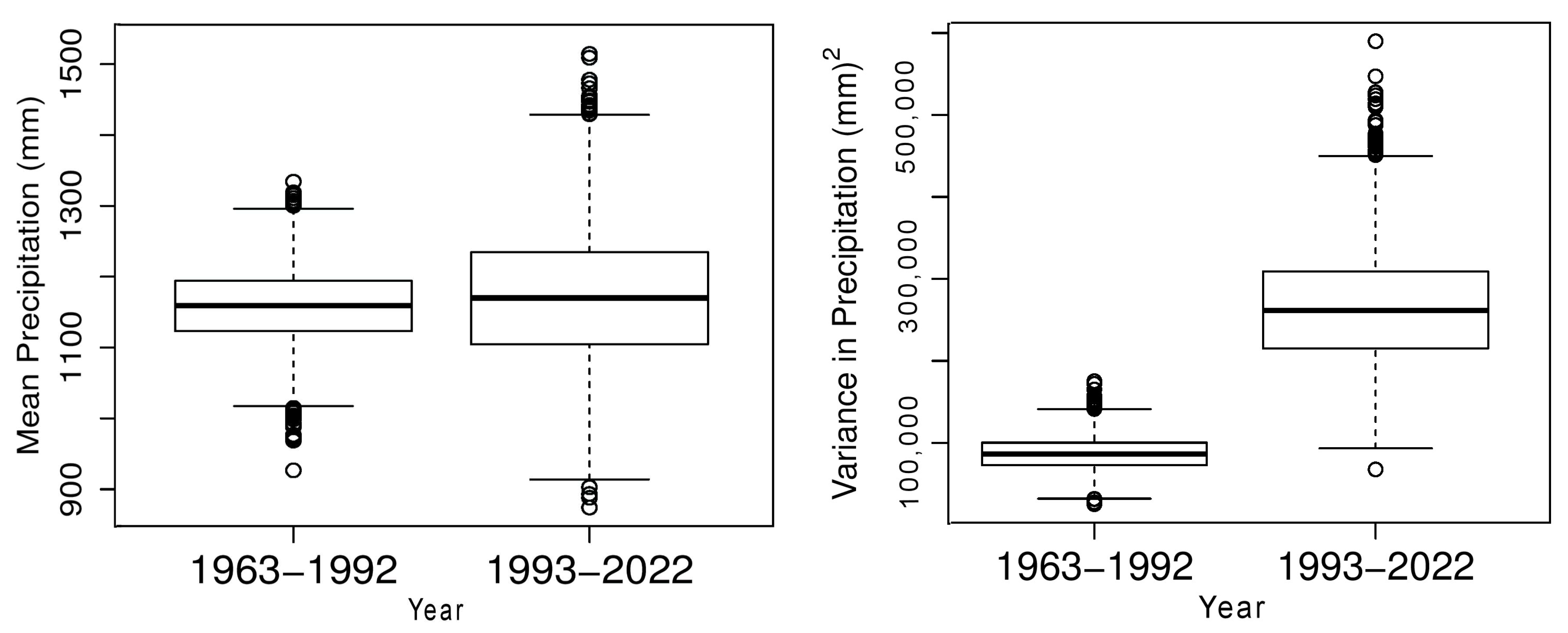
The time series of the 60-year period of May to October rainfall from 1963–2022, for the Upper Hunter region using the observations described in Data Section 2.1, is shown in Figure 3a. The years 2022 and 2023 are highlighted by red boxes. There is a pronounced decrease from well above the 95th percentile (and the second highest recorded in the entire 61-year period) in May to October 2022, down to the 10th percentile in May to October 2023. However, FDs are initiated in a matter of months rather than on a time scale of a year or longer. Notably, in the two months of March and April 2023, the Upper Hunter experienced average to above-average rainfall (Deciles 4–7 and 8–9, respectively). April and May were then followed by Decile 1 rainfall from June until October. Other regions in the state of NSW experienced extreme short-duration rainfall and flash floods in November and December 2023, but at the end of December 2023, the Upper Hunter continued to experience intense drought conditions (Figure 3b).
The Upper Hunter percentile plots in Figure 3a are calculated by totalling the May to October precipitation for the five observing sites, A, S, B, M and RB, shown in Figure 1b–e. They reveal that although there are three major decreases in May–October precipitation, occurring in 1993, 2017 and 2023, the 2023 May–October period was chosen. Following Decile 10 May–October 2022 precipitation (Figure 3a), it also coincided with the dramatic increase in May–October maximum temperature in 2023 to Decile 10, immediately after Decile 1 May–October 2022 maximum temperature (Figure 3c). The mean maximum temperature in Figure 3c is based on the daily maximum temperatures for Scone, as indicated in Figure 1b–e.

3.1.2. Box Plots

The May to October rainfall totals were converted into box plots to illustrate the data distribution for the time periods 1963–1992 and 1993–2022. Figure 4 (left panel) shows that the mean May to October rainfall is similar for both periods. However, there is a clear indication of a significantly larger variance from May to October of 1993–2022, as shown in Figure 4 (right panel).

3.1.3. Permutation Testing

Permutation testing was performed to detect statistically significant differences in the means of the May–October total rainfall time series between the two climate periods 1963–1992 and 1993–2022. As expected from Figure 4, there is no significant difference between the means of the two periods (p-value = 0.91), whereas the difference in the variances is highly significant (p-value = 0.002).

3.1.4. Machine Learning Attribution Results

Attribute selection was conducted for the entire 60-year May–October period 1963–2022. For identification of each climate driver and its index used in Table 1 and Table 2, see Table 3. The rolling window training/test period split begins at 10 years each, with the training period moving forward in time by one year for each model trained, which results in a total of 41 training/test periods. This training/testing period split was selected because the training and testing occur in the consecutive time periods typically designated as pre- and post-accelerated GW [10]. In Table 2a, the mean percentage of the rolling windows for all attributes using the eight different methods is shown in column 10. The six most prominent attributes are highlighted in yellow. SSTs in the equatorial central Pacific Ocean (area Niño3.4) dominate singularly and in combination with GlobalSSTA, the SOI and the IPO. In Table 2a, there is only one dominant attribute, IOD*SAM, that includes SAM for the whole period 1963–2022. However, it is well known that increasingly positive SAM in recent decades has resulted in the circumpolar midlatitude westerlies contracting poleward. Consequently, decreased frontal system rain in the late winter-spring of the southern half of Australia has occurred [20,21]. Therefore, the authors also ran the attribute selection over the two periods 1963–1992 (Table 2b) and 1993–2022 (Table 2c), separately. However, SAM did not appear singularly or in combination as a dominant attribute in the 1993–2022 period at all (Table 3). It did appear singularly and in combination as the top four dominant attributes in the earlier 1963–1992 period (Table 3). Those four leading attributes are SAM, GlobalT*SAM, Niño3.4*SAM and SAM*TSSSTA. This feature, in addition to the fact that all predictors are selected infrequently, as indicated by the mean percentages, is explored further in the following Discussion section.
To avoid overfitting, rolling widows ML always tests the trained ML scheme on unseen data, which should be clear from the addition of the schematic in Figure 2. In addition, we use a range of ML techniques, including SVM and Random Forest with forward and backward selection, because depending on the application, it is not known beforehand which one will be best. In other climate applications of ML, SVM has performed well. In other studies, conducted by the authors, Support Vector Regression has outperformed Random Forest regression [18]. We also note that in this study, two of the SVR schemes also did well, even if not as well as Random Forest Backward selection. The relative performance of the ML schemes supports our comments that, in general, it is not known beforehand what ML scheme might perform best, so employing a wide selection of ML methods is the accepted best approach. Note that the ML methods employed here are statistical regression schemes, i.e., they are not numerical climate prediction models. The ML techniques used here determine the dominant attributes to detect the importance of contributions from the wide range of available climate drivers. The key climate drivers detected by the ML schemes can be used to produce ML prediction models, as shown in previous studies (e.g., [17,22]).

4. Discussion

The most dominant Pacific Ocean and atmospheric attributes, and hence the likely predictors, of May–October Upper Hunter precipitation over the years 1963–2022 seem to be Niño3.4*IPO, Niño3.4*SOI, GlobalSSTA*Niño3.4, Niño3.4, and SOI*IPO. These predictors indicate the dominance of the Walker Circulation combined with increasing central eastern Pacific Ocean equatorial SSTs. A strengthening of the Indian Ocean SST gradient represented by the IOD has also been linked to a stronger Walker Circulation [23]. The IOD*SAM attribute, also found as a likely predictor over 1963–2022, may be linked to the positive SAM and the deep, moist easterly winds combining with anomalous moist SSTs off the northwest coast of Australia during the spring La Niña months of the negative IOD in both La Niña episodes of 2010–12 and 2020–2022. It is noted that La Niña is not a strong indicator of wet conditions, and El Niño is not a strong indicator of dry conditions in some parts of southeast Australia [24], particularly the coastal areas (e.g., [25,26]). However, there are factors contributing to the widespread heavy rain events in most of southeast Australia during November and the summer months of the current El Niño, which can now be discussed in terms of the ML findings and the observed tropospheric circulation changes.
As mentioned above, SAM was a far more dominant attribute during the initial period of 1963–1992 (Table 3). In the later period, 1993–2022, the disappearance of SAM as a predictor can be explained by the observed changes in the SH tropospheric circulation that occurred after the 1990s. Prior to the 1990s, negative 700 hPa anomalies show that the circumpolar westerly winds favoured rain-producing frontal and low pressure systems developed at low mid-latitude and subtropical latitudes across the southern half of Australia and the adjacent Indian Ocean in the cool season months of May–October (Figure 5a). Slight north/south changes in this latitudinal atmospheric pattern imply slight corresponding negative/positive variations in the value of the SAM index. However, the SAM has been trending positive since the 1960s owing to the poleward contraction of the mid-latitude westerly wind belt and the increasing size of the ozone “hole” each spring [27,28,29,30].
Since the 1990s, ozone levels have been recovering [31], while GW has accelerated [10]. As a result, poleward contracted westerly winds are dominated by negative geopotential heights around the Amundsen Sea Low in western SH longitudes. In contrast, there are positive geopotential heights at low mid-latitudes in eastern SH longitudes, particularly in the Australia-New Zealand region (Figure 5b). This pressure imbalance and change in polarity of the geopotential heights around the mid-to-high latitudes of the SH have led to a positive SAM trend in the cool season [31], and the positive pressure anomalies distributed across the southern part of the Australian continent have resulted in the FD of May–October 2023 (Figure 5c). However, the pressure imbalance around the SH with negative geopotential heights in the western SH, partially cancelling out the strongly positive geopotential heights in the eastern SH from the Indian Ocean to the east of New Zealand, explains the absence of SAM attributes since the 1990s. The pressure imbalance is particularly noticeable in November 2023 around the SH mid-latitudes, as shown in Figure 5d.
In November 2023, on the Australian synoptic scale, atmospheric circulation anomalies resulted in a persistent low-pressure trough at 200 hPa linked to Antarctic low pressure and over Australia down through the levels at 500 hPa and 850 hPa (Figure 6a–c), providing a deep, moist layer through southeast Australia, which resulted in outbreaks of heavy rain-producing thunderstorms and localized flooding. Anomalous moisture is evident at 300 hPa in southeast and southwest Australia during November and December 2023 (Figure 6d). The upper trough and subsequent low-pressure development through the middle and low atmospheric levels over Australia were instigated by a branch of the subtropical jet around the apex of the upper trough over Australia into the last week of November. This Antarctic-linked upper low-pressure trough over southeast Australia was slow-moving, trapped between the two anomalous high-pressure centres south of Australia and east of New Zealand (Figure 5d). However, despite record-breaking November rainfall from thunderstorms in parts of inland Eastern Australia, it has not occurred in the Upper Hunter, which remained in drought in late December 2023 (Figure 3b).
Another feature of the ML predictors is the change from those involving the climate driver Niño3.4 before the 1990s to those involving the PMM since the 1990s (Table 3). A locked-phase relationship between PMM and the ENSO lifecycle, especially during strong El Niño events such as 1982, 1997, 2015 and now 2023, suggests a close linkage between ENSO and PMM variability on seasonal to interannual timescales, which is an ongoing area of research [32]. Furthermore, a negative IPO plays a role in the stronger impact of PMM on central Pacific-ENSO since the 1990s [33], requiring that the modulation effects of IPO be considered in understanding the extratropical-tropical climatic connection and ENSO spatial diversity. Note that PMM, IPO and PMM*IPO were all found to be dominant predictors for the more recent period 1993–2023 (Table 3).

5. Conclusions

As the global climate warms, flash droughts are becoming more frequent and more severe. This is particularly true of Australia, which has been identified by the IPCC as being one of the countries at risk from extreme weather and climate events, including flash droughts and flash floods. Here, the authors studied one recent case of a flash drought and identified the key attributes using a range of machine learning techniques. These attributes can be employed in a machine learning prediction scheme and are applicable in combination with high-resolution climate model predictions, especially after the climate model data are downsized to cover specific regions of concern. Finally, it is noteworthy that at the time of writing this article, parts of southern Eastern Australia, including Tasmania, have satisfied the formal definition of a meteorological flash drought, with wet December 2023 and January 2024, followed by a near-record dry February and March 2024.

Author Contributions

Conceptualization, L.M.L. and M.S.; methodology, J.H., L.M.L. and M.S.; software, J.H.; validation, M.S., L.M.L. and J.H.; formal analysis, M.S., J.H. and L.M.L.; investigation, M.S., L.M.L. and J.H.; resources, J.H., M.S.; data curation, J.H.; writing—original draft preparation, M.S. and L.M.L.; writing—review and editing, M.S., L.M.L. and J.H.; visualization, J.H. and M.S.; supervision, L.M.L.; project administration, M.S.; funding acquisition, (no funding). All authors have read and agreed to the published version of the manuscript.

Funding

This research received no external funding.

Data Availability Statement

All data used are available via the web links in the text and references. The precipitation and temperature data are available at http://bom.gov.au/climate/data/, accessed on 7 March 2024.

Acknowledgments

M.S. and L.M.L. acknowledge the School of Mathematical and Physical Sciences, University of Technology for supporting this work.

Conflicts of Interest

The authors declare no conflicts of interests.

References

  1. New South Wales Department of Primary Industry. Combined Drought Indicator. Available online: https://edis.dpi.nsw.gov.au (accessed on 13 March 2024).
  2. Parker, T.; Gallant, A.; Hobbins, M.; Hoffmann, D. Flash drought in Australia and its relationship to evaporative demand. Environ. Res. Lett. 2021, 16, 064033. [Google Scholar] [CrossRef]
  3. NESP. National Environmental and Earth Systems Programme. Earth Systems and Climate Change Hub. Flash Drought in Australia. 30 June 2021. Available online: https://nespclimate.com.au/wp-content/uploads/2021/04/ESCC_Flash-drought_Factsheet.pdf (accessed on 13 March 2024).
  4. Koster, R.D.; Shubert, S.D.; Wang, H.; Mahanama, S.P.; DeAngelis, A.M. Flash drought as captured by reanalysis data: Disentangling the contributions of precipitation deficit and excess evapotranspiration. J. Hydrometeorol. 2019, 20, 1241–1258. [Google Scholar] [CrossRef]
  5. Tyagi, S.; Zhang, X.; Saraswat, D.; Sahany, S.; Mishra, S.K.; Niyogi, D. Flash drought: Review of concept, prediction and the potential for machine learning, deep learning methods. Earth’s Future 2022, 10, e2022EF002723. [Google Scholar] [CrossRef]
  6. Wang, L.; Yuan, X. Two types of flash drought and their connections with seasonal drought. Adv. Atmos. Sci. 2018, 35, 1478–1490. [Google Scholar] [CrossRef]
  7. Otkin, J.A.; Svoboda, M.; Hunt, E.D.; Ford, T.W.; Anderson, M.C.; Hain, C.; Basara, J.B. Flash droughts: A review and assessment of the challenges imposed by rapid-onset droughts in the United States. Bull. Am. Meteorol. Soc. 2018, 99, 911–919. [Google Scholar] [CrossRef]
  8. Jin, C.; Luo, X.; Xiao, X.; Dong, J.; Li, X.; Yang, J.; Zhao, D. The 2012 flash drought threatened US Midwest agroecosystems. Chin. Geogr. Sci. 2019, 29, 768–783. [Google Scholar] [CrossRef]
  9. Bubathi, V.; Leslie, L.; Speer, M.; Hartigan, J.; Wang, J.; Gupta, A. Impact of Accelerated Climate Change on Maximum Temperature Differences between Western and Coastal Sydney. Climate 2023, 11, 76. [Google Scholar] [CrossRef]
  10. IPCC. Climate Change 2022: Impacts, Adaptation, and Vulnerability; Contribution of Working Group II to the Sixth Assessment Report of the Intergovernmental Panel on Climate Change; Pörtner, H.-O., Roberts, D.C., Tignor, M., Poloczanska, E.S., Mintenbeck, K., Alegría, A., Craig, M., Langsdorf, S., Löschke, S., Möller, V., et al., Eds.; Cambridge University Press: Cambridge, UK; New York, NY, USA, 2022; p. 3056. Available online: https://www.ipcc.ch/report/ar6/wg2/ (accessed on 13 March 2024).
  11. Church, J.A.; White, N.J. Sea-level rise from the late 19th to the early 21st century. Surv. Geophys. 2017, 32, 585–602. Available online: http://www.cmar.csiro.au/sealevel/sl_data_cmar.html (accessed on 13 March 2024). [CrossRef]
  12. NOAA (National Oceanic and Atmospheric Administration). Laboratory for Satellite Altimetry: Sea Level Rise. Available online: www.star.nesdis.noaa.gov/sod/lsa/SeaLevelRise/LSA_SLR_timeseries_global.php (accessed on 13 March 2024).
  13. Cheng, L.J.; Abraham, J.; Trenberth, K.E.; Boyer, T.; Mann, M.E.; Zhu, J.; Wang, F.; Yu, F.; Locarnini, R.; Fasullo, J.; et al. New record ocean temperatures and related climate indicators in 2023. Adv. Atmos. Sci. 2024, 1–15. [Google Scholar] [CrossRef]
  14. Speer, M.; Hartigan, J.; Leslie, L. Machine Learning Assessment of the Impact of Global Warming on the Climate Drivers of Water Supply to Australia’s Northern Murray-Darling Basin. Water 2022, 14, 3073. [Google Scholar] [CrossRef]
  15. Canny, J. Combinatorics and Discrete Probability: Stats: Permutation Tests and Bootstrapping [Lecture Notes]; EECS: Berkeley, CA, USA, 2008; pp. 154+196. Available online: https://inst.eecs.berkeley.edu/~cs174/sp08/lecs/index.html (accessed on 13 March 2024).
  16. Wilcox, R.R. Introduction to Robust Estimation and Hypothesis Testing, 5th ed.; Elsevier: Amsterdam, The Netherlands, 2011. [Google Scholar]
  17. Richman, M.B.; Leslie, L.M. Attribution and Prediction of Maximum Temperature Extremes in SE Australia. Procedia Comput. Sci. 2014, 36, 612–617. [Google Scholar] [CrossRef]
  18. Richman, M.B.; Leslie, L.M. Machine Learning for Attribution of Heat and Drought in Southwestern Australia. Procedia Comput. Sci. 2020, 168, 3–10. [Google Scholar] [CrossRef]
  19. Hartigan, J.; MacNamara, S.; Leslie, L.M. Application of Machine Learning to Attribution and Prediction of Seasonal Precipitation and Temperature Trends in Canberra, Australia. Climate 2020, 8, 76. [Google Scholar] [CrossRef]
  20. McKay, R.C.; Boschat, G.; Rudeva, I.; Pepler, A.; Purich, A.; Dowdy, A.; Hope, P.; Gillett, Z.E.; Rauniyar, S. Can southern Australian rainfall decline be explained? A review of possible drivers. WIREs 2023, 14, e820. [Google Scholar] [CrossRef]
  21. Speer, M.S.; Leslie, L.M.; Hartigan, J. Jet Stream Changes over Southeast Australia during the Early Cool Season in Response to Accelerated Global Warming. Climate 2022, 10, 84. [Google Scholar] [CrossRef]
  22. Richman, M.B.; Leslie, L.M. Adaptive Machine Learning Approaches to Seasonal Prediction of Tropical Cyclones. Procedia Comput. Sci. 2012, 12, 276–281. [Google Scholar] [CrossRef]
  23. Funk, C.; Funk, C.; Fink, A.H.; Fink, A.H.; Harrison, L.; Harrison, L.; Segele, Z.; Segele, Z.; Endris, H.S.; Endris, H.S.; et al. Frequent but predictable droughts in East Africa driven by a Walker circulation intensification. Earth’s Future 2023, 11, e2022EF003454. [Google Scholar] [CrossRef]
  24. Tozer, C.R.; Risbey, J.S.; Monselesan, D.P.; Pook, M.J.; Irving, D.; Ramesh, N.; Reddy, J.; Squire, D.T. Impacts of ENSO on Australian rainfall: What not to expect. J. South. Hemisph. Earth Syst. Sci. 2023, 73, 77–81. [Google Scholar] [CrossRef]
  25. Speer, M.S.; Leslie, L.M.; Fierro, A.O. Australian east coast rainfall decline related to large scale climate drivers. Clim. Dyn. 2011, 36, 1419–1429. [Google Scholar] [CrossRef]
  26. McBride, J.L.; Nicholls, N. Seasonal Relationships between Australian Rainfall and the Southern oscillation. Mon. Weather Rev. 1983, 111, 1998–2004. [Google Scholar] [CrossRef]
  27. Arblaster, J.M.; Meehl, G.A. Contributions of external forcings to Southern Annular Mode trends. J. Clim. 2006, 19, 2896–2905. [Google Scholar] [CrossRef]
  28. Gillett, N.P.; Thompson, D.W.J. Simulation of recent Southern Hemisphere climate change. Science 2003, 302, 273–275. [Google Scholar] [CrossRef] [PubMed]
  29. Polvani, L.M.; Waugh, D.; Correa, G.J.P.; Son, S.-W. Stratospheric Ozone Depletion: The Main Driver of Twentieth-Century Atmospheric Circulation Changes in the Southern Hemisphere. J. Clim. 2011, 24, 795–812. [Google Scholar] [CrossRef]
  30. Thompson, D.W.J.; Solomon, S. Interpretation of Recent Southern Hemisphere Climate Change. Science 2002, 96, 895–899. [Google Scholar] [CrossRef] [PubMed]
  31. Zheng, F.; Liu, X.; Wang, H.; Li, Y.; Wang, R.; Yao, S.; Dong, W. Reversing seasonality of Southern Hemisphere Annular Mode trend in the 21st century. Int. J. Climatol. 2023, 43, 6783–6798. [Google Scholar] [CrossRef]
  32. Jiang, F.; Zhang, W.; Boucharel, J.; Jin, F.-F. Tropical origins of the Pacific Meridional Mode associated with the nonlinear interaction of ENSO with the annual cycle. Geophys. Res. Lett. 2023, 50, e2023GL106225. [Google Scholar] [CrossRef]
  33. Liu, B.; Gan, B.; Jia, F.; Wu, L. Impact of the North Pacific Meridional Mode on the Tropical Pacific Modulated by the Interdecadal Pacific Oscillation. J. Clim. 2024, 37, 2199–2216. [Google Scholar] [CrossRef]
Figure 1. Upper Hunter region Eastern Australia showing drought status, rainfall and temperature 2022 and 2023. Map of the State of New South Wales (NSW) in southeast Australia showing, (a) NSW Department of Primary Industries (DPI) combined drought indicator April 2023, (b) New South Wales Department of Primary Industries combined drought indicator for May–October 2023. Note the intense drought in the Upper Hunter region, (c) Decile 10 rainfall May–October 2022 in the Upper Hunter, (d) Decile 1 rainfall May–October 2023, and (e) highest mean maximum temperatures on record May–October 2023 in the Upper Hunter. Rainfall observing stations, Aberdeen—A, Bunnan—B, Muswellbrook—M, Rouchel Brook—RB and Scone—S are marked on (be).
Climate 12 00049 g001
Figure 2. Schematic diagram of the ML training/test method. W = the training window; h = the test window; S = the size of the rolling window step, and N is the total number of training/test windows. In this 60-year study, which starts in 1963, W = 10, h = 10, S = 1 and N = 41.
Climate 12 00049 g002
Figure 3. Total Precipitation, maximum temperature time series 1963–2023 and drought status in December 2023. (a) Total precipitation time series, May–October 1963–2023, for Aberdeen—A, Bunnan—B, Muswellbrook—M, Rouchel Brook—RB and Scone—S. Solid black line is total May–October precipitation 1963–2022 for all stations. Dashed lines are 5th and 95th percentiles (red), 10th and 90th percentiles (orange), 15th and 85th percentiles (light blue), 20th and 80th percentiles (brown), 25th and 75th percentiles (dark blue), and solid black line is the median. Open red squares show May–October 2022 is Decile 10 (very much above average) and May–October 2023 is Decile 1 (very much below average), (b) mean TMax time series May–October 1963–2023 are Upper Hunter daily observations for Scone. Dashed lines are 5th and 95th percentiles (bottom and top red), 10th and 90th percentiles (bottom and top orange), 15th and 85th percentiles (bottom and top light blue), 20th and 80th percentiles (bottom and top brown), 25th and 75th percentiles (bottom and top dark blue), and the horizontal solid black line is the median. Open red square shows May–October 2022 is Decile 1 (very much below average), and May–October 2023 is Decile 10 (and highest recorded), (c) New South Wales DPI combined drought indicator, 31 December 2023, shows the Upper Hunter experiencing drought with some areas in intense drought.
Climate 12 00049 g003
Figure 4. Box and whisker plots of mean precipitation. Box-whisker plots of mean precipitation (left panel) for the consecutive periods 1963–1992 and 1993–2022 (left panel) and variance (right panel), for the Upper Hunter. The inter-quartile range, from the 25th and 75th percentiles, is represented by the horizontal lines of the boxes, with the medians (50th percentiles) are shown as thick, horizontal black lines. The lower horizontal lines are the 10th percentiles and the upper horizontal lines near the outliers are 90th percentiles. The circles above and below the 10th and 90th percentile lines are the outliers.
Climate 12 00049 g004
Figure 5. Southern Hemisphere tropospheric circulation anomalies. NCEP/NCAR Reanalysis 700 hPa geopotential height (m) composite anomalies May–October for, (a) 1963–1992, (b) 1993–2023, (c) 2023, and November for, (d) 2023.
Climate 12 00049 g005aClimate 12 00049 g005b
Figure 6. Synoptic geopotential and southern hemispheric relative humidity tropospheric circulation anomalies. Australian Bureau of Meteorology November 2023 ACCESS model anomalies at, (a) 200 hPa, (b) 500 hPa, (c) 850 hPa, and November-December 2023 NCEP/NCAR Reanalysis relative humidity (%) composite anomalies, (d) at 300 hPa. ACCESS model anomalies are available at: http://www.bom.gov.au/jsp/awap/cmb/achive.jsp?level=mslp&map=mean&area=nat (accessed on 7 March 2024).
Climate 12 00049 g006
Table 1. Identification of climate drivers with their acronyms and indices used.
Climate DriverClimate Driver Acronym
Atlantic Multi-decadal OscillationAMO
Indian Ocean Dipole or Dipole Mode IndexIOD
Global Sea-surface temperature anomalyGlobalSSTA
Global TemperatureGlobalT
Nino3 and Nino4 SST areas; equatorial central eastern Pacific OceanNiño3.4
Pacific Meridional Mode—SST anomaly component of indexPMM
Southern Annular ModeSAM
Southern Oscillation IndexSOI
Interdecadal Pacific Oscillation or Pacific Decadal OscillationIPO
Tasman Sea-sea surface temperature anomalyTSSSTA
Table 2. (a) Attribute/Predictor selection for Upper Hunter precipitation data 1963–2022 using the eight different ML techniques. The percentage of rolling windows times series selection of the attributes is shown for each of the eight methods (columns 2–9). The mean and standard deviation for rows and columns, are shown. The six most dominant attributes and hence likely predictors are highlighted (yellow). (b) Attribute/Predictor selection for Upper Hunter precipitation data 1963–1992 using the eight different ML techniques. The percentage of rolling windows time series selection of the predictors ≥45% is shown for each of the eight methods (columns 2–9). The mean and standard deviation are shown for all rows and columns. The six most dominant attributes are highlighted (yellow). (c) Attribute/Predictor selection for Upper Hunter precipitation data 1993–2022 using the eight different ML techniques. The percentage of rolling windows time series selection of predictors ≥45% is shown for each of the eight methods (columns 2–9). The mean and standard deviation for rows and columns is shown. The seven most dominant predictors are highlighted (yellow).
(a)
MACHINE LEARNING TECHNIQUES
ATTRIBUTESLR FSVM RBF FSVM Poly FRF FLR BSVM RBF BSVM Poly BRF BMeanStd. Dev.
AMO9.7617.0753.6621.9531.7112.2019.5195.1232.6228.83
IOD9.7626.8368.2939.0229.279.7653.6697.5641.7730.22
GlobalSSTA14.6331.7160.9819.5124.3919.5160.9890.2440.2427.25
GlobalT2.4436.5970.7334.1531.7119.5148.7895.1242.3829.18
Niño3.44.8856.1078.0551.2241.4626.8331.7197.5648.4829.40
PMM4.8834.1558.5429.2739.0221.9563.4197.5643.6028.81
SAM19.5141.4648.7853.6648.7814.6336.5992.6844.5124.00
SOI9.7658.5475.6131.7126.8312.2060.9892.6846.0430.39
IPO19.5153.6678.0541.4631.714.8829.2797.5644.5130.76
TSSSTA7.3231.7156.1021.9524.397.3217.0787.8031.7127.50
AMO*IOD4.8817.0770.7343.9017.079.7648.7895.1238.4132.19
AMO*GlobalSSTA17.074.8836.5917.0736.592.4458.5485.3732.3228.41
AMO*GlobalT7.3212.2068.2917.0734.150.0068.2997.5638.1135.63
AMO*Niño3.412.2034.1568.2929.2721.9512.2043.9092.6839.3328.31
AMO*PMM4.8836.5960.9831.7136.5919.5139.02100.0041.1628.72
AMO*SAM34.1524.3939.0231.7136.5921.9568.2997.5644.2125.79
AMO*SOI9.769.7665.8519.5112.200.0031.7195.1230.4933.11
AMO*IPO19.5134.1560.9839.0224.392.4434.1597.5639.0229.01
AMO*TSSSTA4.8819.5173.1729.2721.957.3243.9097.5637.2032.79
IOD*GlobalSSTA41.4619.5173.1741.4653.662.4436.5995.1245.4329.12
IOD*GlobalT36.5924.3970.7341.4646.3412.2043.9095.1246.3426.04
IOD*Niño3.40.0060.9863.4160.989.7629.2746.3497.5646.0431.89
IOD*PMM21.9517.0768.2929.274.880.0048.78100.0036.2834.16
IOD*SAM14.6365.8570.7348.7812.2039.0243.9097.5649.0928.72
IOD*SOI17.0743.9073.1741.4612.207.3260.9897.5644.2131.84
IOD*IPO4.8836.5963.4148.784.889.7670.7390.2441.1632.68
IOD*TSSST2.4424.3956.1046.344.884.8824.3992.6832.0131.46
GlobalSSTA*GlobalT4.8831.7156.1029.277.3226.8351.2295.1237.8029.38
GlobalSSTA*Niño3.44.8858.5458.5468.2917.0743.9036.59100.0048.4830.00
GlobalSSTA*PMM31.7119.5141.4648.7826.834.8846.3492.6839.0226.14
GlobalSSTA*SAM14.6314.6348.7829.2719.510.0043.9097.5633.5430.46
GlobalSSTA*SOI9.7648.7856.1036.592.4441.4653.6697.5643.2929.49
GlobalSSTA*IPO9.7651.2260.9846.3414.6329.2734.1590.2442.0726.20
GlobalSSTA*TSSSTA26.8324.3941.4626.839.7619.5148.7890.2435.9825.07
GlobalT*Niño3.47.3258.5448.7863.412.4429.2748.7895.1244.2130.56
GlobalT*PMM4.8829.2758.5443.9017.079.7656.1095.1239.3330.34
GlobalT*SAM34.1531.7148.7846.342.4436.5941.4697.5642.3826.49
GlobalT*SOI29.2736.5953.6629.2721.9512.2063.4192.6842.3826.20
GlobalT*IPO4.8856.1063.4158.5412.2031.7146.3497.5646.3429.90
GlobalT*TSSSTA21.9514.6351.229.762.4412.2063.4187.8032.9330.77
Nino3.4*PMM12.2046.3468.2929.277.3217.0734.1590.2438.1128.92
Nino3.4*SAM26.8358.5463.4148.780.0029.2743.9092.6845.4327.81
Nino3.4*SOI21.9560.9878.0534.159.7631.7158.5497.5649.0929.83
Nino3.4*IPO17.0773.1773.1746.347.3241.4663.4197.5652.4430.38
Niño3.4*TSSSTA21.9541.4670.7336.590.0041.4629.2795.1242.0729.29
PMM*SAM21.9529.2758.5426.830.009.7634.1597.5634.7630.71
PMM*SOI2.4429.2765.8531.710.009.7629.2792.6832.6232.14
PMM*IPO17.0746.3470.7324.390.0024.3953.6695.1241.4631.18
PMM*TSSSTA14.6326.8360.9831.710.0034.1534.15100.0037.8030.60
SAM*SOI43.9046.3456.1026.830.009.7646.3497.5640.8530.12
SAM*IPO14.6353.6673.1748.780.0021.9553.6695.1245.1231.51
SAM*TSSSTA39.0224.3953.6631.710.0026.8348.7897.5640.2428.44
SOI*IPO36.5968.2968.2929.270.0039.0248.7887.8047.2627.44
SOI*TSSSTA21.9517.0756.1031.710.009.7629.2795.1232.6230.27
IPO*TSSSTA26.8339.0256.1041.460.0021.9541.4687.8039.3325.76
Mean16.3636.5461.6936.6716.3618.0945.7694.86
Standard Deviation11.4116.8410.2312.3715.0612.6812.793.56
(b)
MACHINE LEARNING TECHNIQUES
ATTRIBUTESLR FSVM RBF FSVM Poly FRF FLR BSVM RBF BSVM Poly BRF BMeanStd. Dev.
GlobalT9.0927.2790.919.0981.820.0045.45100.0045.4540.36
SAM36.3663.6427.2754.5590.910.0027.27100.0050.0034.02
TPI27.2718.18100.0018.1872.730.0027.27100.0045.4539.48
IOD*GlobalT45.4563.6481.8236.360.0036.3636.36100.0050.0031.11
IOD*SAM0.0081.8272.7345.450.0054.5527.27100.0047.7336.93
GlobalSSTA*GlobalT9.0972.7336.3654.550.0063.6436.3690.9145.4531.11
GlobalT*SAM36.3690.9154.5563.640.0072.7336.36100.0056.8232.51
GlobalT*TPI0.0063.6463.6463.640.0054.5545.4590.9147.7332.14
Nino3.4*SAM18.1890.9154.5590.910.0054.5527.27100.0054.5537.32
Nino3.4*TPI9.0972.7372.7345.450.0045.4536.36100.0047.7333.58
SAM*TSSSTA45.4572.7354.559.090.0063.6463.64100.0051.1432.93
SOI*TPI27.2772.7372.739.090.0072.7381.8290.9153.4135.52
Mean21.9665.9165.1541.6620.4543.1840.9097.72
Standard Deviation16.6522.3121.1726.1337.2027.9816.674.11
(c)
MACHINE LEARNING TECHNIQUES
ATTRIBUTESLR FSVM RBF FSVM Poly FRF FLR BSVM RBF BSVM Poly BRF BMeanStd. Dev.
AMO9.0918.1872.7363.6454.550.0054.5590.9145.4532.60
IOD27.2754.5563.6454.5563.6436.3654.55100.0056.8221.60
GlobalT0.0036.3681.8254.5545.450.0063.6490.9146.5933.82
Niño3.49.09100.0081.82100.0045.459.0945.45100.0061.3639.40
PMM9.0954.5572.7363.6481.820.00100.0090.9159.0936.69
SOI0.0054.5572.7318.1872.7318.1845.45100.0047.7333.93
TPI9.0990.9181.8245.4572.739.0945.45100.0056.8235.29
TSSSTA27.2718.1881.8236.3663.6427.2727.27100.0047.7330.25
AMO*IOD27.2718.1890.9154.5572.7336.3636.3690.9153.4128.52
AMO*SAM0.0045.4572.7336.3636.360.0081.82100.0046.5936.51
AMO*TSSSTA27.2718.1863.6463.649.099.0972.73100.0045.4534.02
IOD*GlobalT36.3618.1872.7354.550.000.0081.82100.0045.4537.95
IOD*Niño3.418.1854.5572.7354.550.0036.3663.6490.9148.8629.53
IOD*SOI18.1872.7372.7363.640.009.0963.6490.9148.8634.34
IOD*TPI27.2727.2781.8254.550.009.0972.73100.0046.5936.18
GlobalSSTA*Niño3.40.00100.0072.7345.450.0090.9127.27100.0054.5542.36
GlobalT*Niño3.49.0990.9136.3672.730.0081.820.00100.0048.8642.34
Nino3.4*PMM27.2781.8281.8263.640.009.0963.64100.0053.4136.83
Nino3.4*TPI0.00100.0081.8263.640.0045.4554.5590.9154.5538.26
PMM*SOI0.0081.8272.7363.640.009.0945.45100.0046.5939.31
PMM*TPI0.0063.6490.9163.640.0036.3690.91100.0055.6839.90
SAM*TPI72.7336.3672.7354.550.009.0954.55100.0050.0033.67
Mean16.1156.1974.7956.6128.0921.8956.6197.10
Standard Deviation17.5029.9011.1915.6032.2225.3527.784.33
Table 3. The six most dominant attributes/predictors for the two periods 1963–1992 and 1993–2023. The symbol } indicates equal percentages.
Predictors
1963–2023
Predictors
1963–1992
Predictors
1993–2023
Niño3.4*TPI }GlobalT*SAMNiño3.4
IOD*SAM }Niño3.4*SAMPMM
Niño3.4*SOISOI*IPOIOD }
GlobalSSTA*Nino3.4 }SAM*TSSSTAIPO }
Niño3.4 }SAM }PMM*IPO
SOI*IPOIOD*GlobalT }GlobalSSTA*Niño3.4
Disclaimer/Publisher’s Note: The statements, opinions and data contained in all publications are solely those of the individual author(s) and contributor(s) and not of MDPI and/or the editor(s). MDPI and/or the editor(s) disclaim responsibility for any injury to people or property resulting from any ideas, methods, instructions or products referred to in the content.

