Review

Applying Machine Learning in Numerical Weather and Climate Modeling Systems

by
Vladimir Krasnopolsky
Environmental Modeling Center, National Centers for Environmental Predictions, College Park, MD 20740, USA
Climate 2024, 12(6), 78; https://doi.org/10.3390/cli12060078
Submission received: 21 March 2024 / Revised: 22 May 2024 / Accepted: 23 May 2024 / Published: 26 May 2024
(This article belongs to the Special Issue Addressing Climate Change with Artificial Intelligence Methods)

Abstract

:
In this paper major machine learning (ML) tools and the most important applications developed elsewhere for numerical weather and climate modeling systems (NWCMS) are reviewed. NWCMSs are briefly introduced. The most important papers published in this field in recent years are reviewed. The advantages and limitations of the ML approach in applications to NWCMS are briefly discussed. Currently, this field is experiencing explosive growth. Several important papers are published every week. Thus, this paper should be considered as a simple introduction to the problem.

1. Introduction

Everything we think we know about the world is a model
Our models do have a strong congruence with the world
Our models fall far short of representing the real world fully.
Donella H. Meadows [1]
At the end of the Second World War, the field of numerical weather and climate modeling developed as a collection of simple linear or weakly nonlinear single-disciplinary models, such as simplified atmospheric and oceanic models, that included a limited description of the physical processes. However, a well-pronounced trend has emerged in numerical weather and climate modeling over the last several decades. It marks a transition to complex, nonlinear, multidisciplinary systems or numerical weather/climate modeling systems (NWCMS) like the European Centre for Medium-Range Weather Forecasts (ECMWF) models (e.g., Integrated Forecasting System (IFS)), National Oceanic and Atmospheric Administration (NOAA) National Centers for Environmental Prediction (NCEP) Global Forecast System (GFS) and Climate Forecast System (CFS), NCEP Seasonal Forecast System (SFS), and NOAA Unified Forecast System (UFS), with fully coupled atmosphere, land, ocean, ice and wave components [2,3], etc.
Any NWCMS usually has, as three major subsystems, the following three important components: (1) a data assimilation system (DAS)—a subsystem that ingests/assimilates data, and prepares initial conditions, necessary to run the model; (2) a statistical or deterministic (based on first principles equations) model that includes model dynamics (dycor) and model physics (here terms “physics” includes all physical, chemical, and biological processes that are incorporated into the model); and (3) a post-processing (PP) subsystem that corrects model outputs, using data.
Currently, NWCMSs face four major challenges:
  • The vast amounts of observational data available from satellites, in situ scientific measurements, and in the future, from Internet-of-Things devices, increase with tremendous speed. Even now, only a small percentage of the available data is used in modern DASs. The problems with the assimilation of new data in DASs range from increased time consumption (with increasing amounts of data) vs. limited computational resources to the necessity of new approaches for assimilating new types of data [4,5];
  • The increasing requirements to improve the accuracy and the forecast horizon of numerical weather/climate modeling systems are leading to their growing complexity, due to increasing horizontal and vertical resolutions and the related complexity of model physics. Thus, global and regional modeling activities consume a tremendous amount of computing resources, which presents a significant challenge despite growing computing capabilities. Model ensemble systems have already faced the computational resources problem that limits the resolution and/or the number of ensemble members in these systems [5];
  • Model physics is the most computationally demanding part of numerical weather/climate modeling systems. With the increase in model resolutions, many subgrid physical processes that are currently parameterized become resolved processes and should be treated correspondingly. However, the nature of these processes is not always sufficiently understood to develop a description of the processes based on first principles. With the increase in model resolution, the scales of the subgrid processes that should be parameterized become smaller and smaller. Parameterizations of such processes often become more and more time-consuming and sometimes less accurate because the underlying physical principles may not be fully understood [4,5];
  • Current NWCMSs produce improved forecasts with better accuracy. A major part of these improvements is due to the increase in supercomputing power that has enabled higher model resolution, better physics/chemistry/biology description, and more comprehensive data assimilation [5]. Yet, the “demise of the ‘laws’ of Dennard and Moore” [6,7] indicates that this progress is unlikely to continue, due to an increase in the required computer power. Moore’s law drove the economics of computing by stating that every 18 months, the number of transistors on a chip would double at an approximately equal cost. However, the cost per transistor starts to grow with the latest chip generations, indicating an end to this law. Thus, due to the aforementioned limitations, results produced by NWCMSs still contain errors of various natures. Thus, the PP correction of model output errors becomes even more important [8]. Currently used in NWP operational practices, post-processing systems like Model Output Statistics (MOS) [9] are based on linear techniques (linear regressions). However, because optimal corrections of model outputs are nonlinear, correcting the biases of even regional fields requires the introduction of many millions of linear regressions in MOS [10,11], making such systems cumbersome and resource-consuming.
Flexible and powerful numerical techniques are required to reduce the growing demands for computer resources that outrun the actual growth of computer power, enable new data types to be used, meet the challenges of model physics, and develop flexible PP techniques to correct errors in model outputs. Developments in the various fields of artificial intelligence (AI), in particular, in machine learning (ML), computer science, and statistics have indicated the possibilities of using ML as one of these techniques. For example, ML is increasingly being applied to solve and/or alleviate problems in NWCMSs [12,13,14,15,16].

2. ML for NWCMSs Background
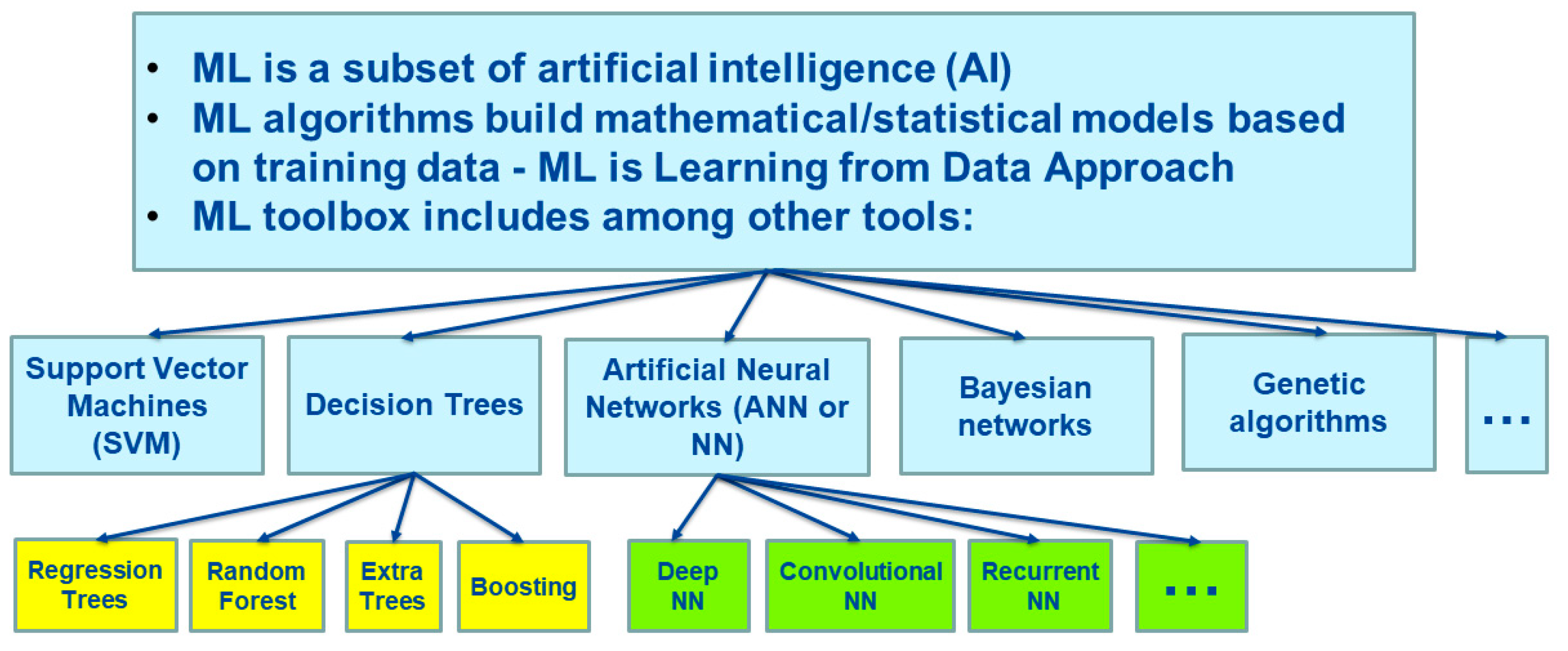
Machine learning is a subfield of AI that uses statistical techniques to give computers the ability to “learn” (i.e., progressively improve performance on a specific task) from data, without being explicitly programmed [17]. This definition explains why ML is sometimes also called statistical learning or learning from data [18].

2.1. ML Tools

ML algorithms build a model based on sample data, known as training data, to make predictions or decisions without being explicitly programmed to do so [14]. Then, these ML models can be used for representing, interpolating, and limited extrapolating of the data. The set of ML tools includes a large variety of different algorithms such as various neural networks (NN), different kinds of decision trees (e.g., random forest algorithms), kernel methods (e.g., support vector machines and principal component analysis), Bayesian algorithms, etc. (see Figure 1). Some of these algorithms are more universal (e.g., generic multilayer perceptron or NNs), and some are more focused on a specific class of problems (e.g., convolutional NNs that show an impressive performance as image/pattern recognition algorithms).
There are many different types of NNs: shallow, deep, convolutional, recurrent, etc., as well as many types of tree algorithms (see Figure 1). Here, we briefly discuss two major types of ML tools that have been applied to develop applications for numerical weather and climate prediction systems: (1) NNs that have been applied in most studies (e.g., [19,20,21,22,23]); and (2) tree algorithms that have been applied in a few works [24,25].
Most applications proposed in the aforementioned works are based on two assumptions:
5.
Many NWCMS applications, from a mathematical point of view, may be considered as mapping, M, that is a relationship between two vectors or two sets of parameters X and Y, as follows:
Y = M X ,         X R n ,   Y R m  
where n and m are the dimensionalities of vectors X and Y correspondingly.
6.
ML provides an all-purpose non-linear fitting capability. NN, the major ML tool that is used in applications, are “universal approximators” [26] for complex multidimensional nonlinear mappings [27,28,29,30,31]. Such tools can be used, and have already been used, to develop a large variety of applications for NWCMSs.
A generic NN that is used for modeling/approximating complex nonlinear multidimensional mappings is called the multilayer perceptron. It is comprised of “neurons” that are arranged in “layers”. A generic neuron can be expressed as follows:
x j n + 1 = ϕ b j n + i = 1 k n a j i n ·   x i n
Equation (2) represents a neuron number j in the layer number n. x j n + 1 is the output of the neuron that, at the same time, is an input to neurons of the layer number n+1. Here, x j n are inputs to neurons of the layer number n (outputs of neurons of the layer number n−1, the input layer corresponds to n = 0), a and b are fitting parameters or NN weights and biases, ϕ is the so-called activation function, and kn is the number of neurons in the layer number n. The entire layer number n can be represented by a matrix equation as follows:
X n + 1 = ϕ B n + A n · X n
where for n = 0, Xn = X, a vector of the NN inputs. If the layer number n+1 is the output layer, linear neurons are often used for the output layer,
Y = X n + 1 = B n + A n · X n
where Y is a vector of outputs.
The activation function ϕ is a nonlinear function (see Figure 2), often specified as the hyperbolic tangent; however, rectangular linear unit, SoftMax, leaky rectangular linear unit, Gaussian, trigonometric functions, etc. are also used in applications [14]. All layers of the multilayer perceptron NN between input and output layers are called “hidden layers”. NNs with multiple hidden layers are called “deep neural networks” (DNN). The simplest multilayer perceptron NN with one hidden layer is called a “shallow” NN (SNN). SNN is a generic analytical nonlinear approximation or model for mapping (1) and a mathematical solution of the ML problem [27,28,29]. Multiple authors have shown, in a variety of contexts, that the SNN can approximate any continuous or almost continuous (with a finite number of finite discontinuities) mapping (1) [22,30,31,32]. The accuracy of the SNN approximation, or the ability of the SNN to resolve details of the mapping (1), is proportional to the number of neurons k in the hidden layer [33].
Additional hidden layers and/or nonlinear neurons in the output layer can be introduced and the resulting DNN can be applied to either mapping approximation problems or problems of a different nature. DNNs have been extremely successful in many areas, including in applications for numerical weather/climate modeling systems. However, as pointed out by Vapnik [29], from the standpoint of statistical learning theory, only SNN has been formally shown to be a solution to the mapping approximation problem (see also Figure 3). Successful approximation of the mapping (1) by a DNN cannot be guaranteed theoretically, and this specific application of DNNs should be considered a heuristic approach. Both SNNs and DNNs have been successfully applied to numerical weather/climate modeling system mappings by different authors (see discussion in the following Sections).
NNs are very successful in solving complex nonlinear mapping problems. After they are trained, their application is fast; they are easily parallelizable. They use the training dataset only during training. Trained NNs contain all necessary information about the mapping in a set of NN weights and biases that is usually much smaller than the training set and does not require a lot of memory. However, NNs are difficult to interpret because information about the mapping is distributed over multiple weights and biases, which is typical for any nonlinear statistical model. Additionally, as with any nonlinear statistical model, NN has limited ability for prediction/extrapolation/generalization; however, a well-trained NN is capable of a limited accurate generalization.
A decision tree is a tree-like model of decisions and their consequences. They are widely used in statistics and ML for solving non-linear classification and regression problems. Decision trees are easily interpretable; however, they are not stable to noise in the data. To avoid instabilities and improve the accuracy and robustness of the approach, an ensemble of decision trees called a ‘forest’ approach, has been developed. Introducing elements of randomness to the trees turned out to be beneficial, hence the approach is named “random forest” [34]. This algorithm has many advantages: it does not require complex pre-processing and normalization of data; it easily handles missing data; the random forest is a robust algorithm that can handle noisy data and outliers. However, random forests require more memory than other algorithms because this algorithm stores multiple trees. This can be a problem if the dataset is large. To apply a trained random forest algorithm, the entire training set must be kept in memory. In addition, it will not be able to predict any value outside the available training set values, since averaging various trees, each of which is built upon the training set, is a big part of random forest models. Thus, we cannot expect reliable predictions/extrapolations/generalizations when using the random trees algorithm. For more detailed discussions of NN, trees, and other ML tools, see [14].

2.2. ML for NWCMS Specifics

It is critical to understand that the development of many ML applications for numerical weather and climate modeling systems is essentially different to the standard ML approach. First, a standard ML approach consists of two major steps: (1) training an ML tool (e.g., an NN) using training and test sets; and (2) validating a trained tool on an independent validation set. If the validation is successful, the tool is ready for use. In this sense “Generative AI” (like ChatGPT)—deep learning models that can generate high-quality text, images, and other content based on the data they were trained on—can be considered a traditional ML application.
When an ML application is being developed for a numerical weather modeling system to work within the model or in the model environment (e.g., data assimilation system), in close connection with the model, the third and the most important validation step must be included in the approach: (3) the trained application should be introduced in the model to check its coherence with the model and the model environment, to check that it does not introduce any disruption in the stable functioning of the modeling system and that the system keeps producing meaningful results.
Second, such applications usually do not use unstructured datasets (sets that consist of a mixture of numerical, text, images, etc.) for training and validation. Usually, structured datasets that consist of matrixes or tables of numerical observations or simulated data are used.
Third, generally, there are not enough observations for the training and validation of ML applications for NWCMSs. The observations in weather and climate systems are usually sparse and located close to the land and ocean surface. Thus, observations are very often augmented by data simulated by numerical models. Analysis and reanalysis, which are thoroughly fused observations and data simulated by numerical models, are often used.
It is noteworthy that the use of a relatively large number of mostly uninterpretable parameters led to the perception of ML as a “black box” approach, which created problems with its acceptance by weather and climate modelers. In essence, the trade-off between simple statistics and ML is mostly between interpretability and accuracy. With relatively few parameters and few predictors (often by using predictor selection methods to reduce the number of predictors), simple statistical models are generally much more interpretable than ML models.
Most ML tools are closely related to nonlinear nonparametric statistics. A limitation of the parametric approach is that the functional form for the statistical model is specified, which may not work well for some datasets. For example, a linear regression model may not work for data representing essentially nonlinear behavior. The alternative non-parametric modeling approach still has parameters, but the parameters are not used to control the specified functional form of the model; instead, the parameters are used to control the model complexity. Thus, in principle, a nonparametric approach (and ML approach as well) is more flexible, and a nonparametric/ML model can automatically adjust to/learn any nonlinear behavior exhibited by data. On the other hand, parametric models (if they work well) may be easier to interpret. With nonparametric/ML models, such a straightforward interpretation is not possible.
For example, coefficients of linear regression models may be interpreted as contributions of the corresponding input variables into the output variable. In contrast, ML methods, such as neural networks and random forests, are run as an ensemble of models initialized with different random numbers, leading to a vast number of parameters that are largely uninterpretable. In this case, the contributions of an input parameter are distributed through multiple coefficients of the nonlinear nonparametric/ML model. Over time, datasets become increasingly larger and more complex, making good interpretability harder to achieve even with parametric statistical models. At the same time, the advantage in prediction accuracy attained by ML models makes them more and more attractive. Currently, a lot of works have been published that are devoted to the problem of the interpretability of ML models [35].

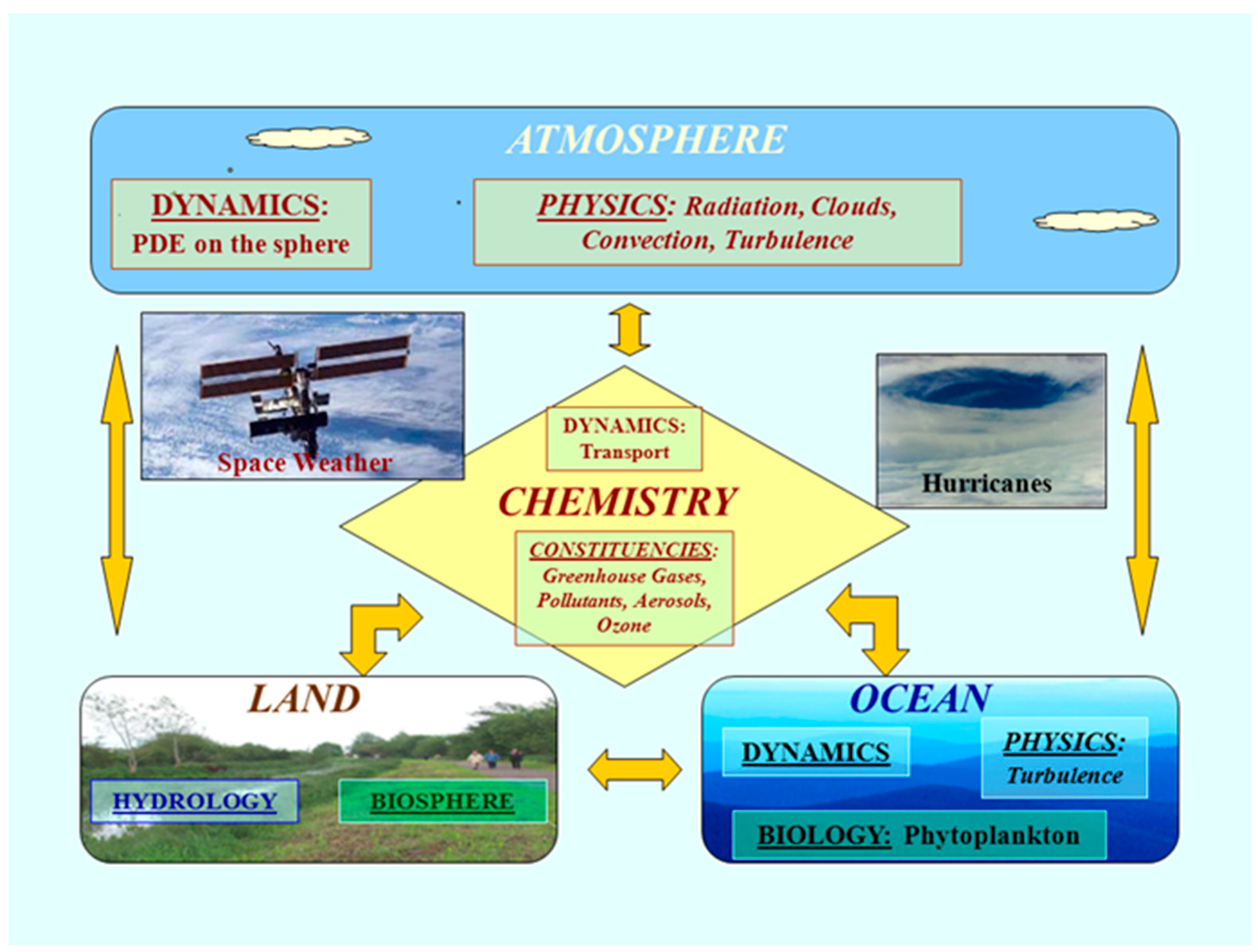
3. Climate and Weather Systems

3.1. Systems and Subsystems

Formally, a system can be defined as a set of elements or parts that is coherently organized and interconnected in a pattern or structure that produces a characteristic set of behaviors, often classified as its “function” or “purpose” [1]. Thus, any system is composed of components or parts. In aggregations, parts are added; in systems, components or parts are arranged or organized; hence, each system has a well-defined structure. Systems are significant because of organization–positional values, and because of their structure. If a system is properly structured or organized, then it is more than the total sum of its parts and the whole system may demonstrate behavior (quality) that cannot be predicted by the behavior of its parts. In such cases, we are talking about a synergy of the parts in the system.
In a complex climate and weather system (see Figure 4), the atmospheric constituent (as well as other ones) of the system is itself a complex system of interacting dynamical, physical (radiation, convection, etc.), and chemical processes (see Figure 4). Such constituent parts of the whole system that themselves have a structure (organization) are called subsystems. Systems arranged in such a way (nested systems in the system) are called hierarchical systems [36,37]. A hierarchical system is an arrangement of subsystems, in which the subsystems are represented as being “above”, “below”, or “at the same level as” with respect to one another. In such a hierarchy, subsystems can interact either directly or indirectly, and either vertically (between different levels of hierarchy) or horizontally (at the same level). The number of vertical levels determines the depth or the vertical (hierarchical) complexity of the hierarchical system [37].
Interactions and relationships at a higher level of hierarchical complexity organize and transform the lower-order interactions, producing organizations of lower-order relationships that are new and not arbitrary and cannot be accomplished by those lower-order interactions alone (outside of the system). The higher-order relationship governs or coordinates the relationships of the next lower order; it embraces and transcends the lower orders. It is noteworthy that interactions in complex systems are better described by feedback loops than by one directional cause-and-effect type actions, which makes the analysis of such systems even more difficult.

3.2. ML for NWCMS and Its Subsystems

Figure 5 portrays a NWCMS with subsystems. All subsystems shown in the figure and the entire system, from the mathematical point of view, are mappings—relationships between the vector of output parameters and the vector of input parameters, like (1). This is why ML methods apply to NWCMS and subsystems.
NOAA and ECMWF scientists were among the pioneers in the field of ML applications to NWCMS. They first developed many key approaches that are currently used in this field. NOAA developments in this field during the period 1995 to 2012 are reviewed in [15]. Later developments are presented in [38,39].
Currently, ML is considered a powerful and prospective tool for the further development and improvement of NWCMSs at ECMWF [40] (see also Figure 5), UKMO and other world weather centers. According to the NOAA AI Strategy, it is expected that the ML applications briefly described below will be developed at NWS in close collaboration with the Academy, NOAA Cooperative Institutes, NOAA Cooperative Science Centers, other NOAA divisions, private companies, and international communities.
Figure 5. ML applications at ECMWF that are already being explored or planned. The color-coding of the boxes corresponds to the respective component of the workflow for NWP (from [40]).
Climate 12 00078 g005
Two major types of ML tools have been applied to develop applications for NWCMS: (1) NNs [21,23,41,42] and (2) tree algorithms [24,25]. There are many different types of NNs: shallow, deep, convolutional, recurrent, etc., as well as many types of tree algorithms (see Figure 1). The advantages and limitations of different types of ML are discussed in detail in [38] and in Section 2 of this paper.

4. Hybridization of ML with Traditional Numerical Modeling

Initially, ML methods were introduced into weather and climate science as nonlinear statistical models to improve upon linear statistical tools. In the beginning, ML weather and climate applications had no direct relation to numerical models based on first-principle dynamic equations and physics (here we use the term “physics” in the broadest sense that includes physics, chemistry, and biology). Only at the beginning of the 2000s did the convergence and hybridization of the two entirely different approaches, ML and numerical modeling, start [19,20], pointing to a new future for weather and climate science.

4.1. ML for Data Assimilation

Both DAS and ML, from a mathematical point of view, belong to the same class of optimization problems. Both methods apply a nonlinear optimization of an error function to determine the optimal parameters of the system. Because DAS can be considered as a mapping between observations, first guess, and the final analysis, in principle, it may be possible to substitute the entire variational DAS with an ML DAS [30,43]. However, while, and if, this approach is reaching maturity, it makes sense to focus on using ML for improvements in the existing variational DASs. The following elements of the variational DAS are good candidates for applying ML.

4.1.1. Fast ML Forward Models for Direct Assimilation of Satellite Measurements

Forward models (FM) are used for direct assimilation of satellite radiances in DAS [44]. FMs are usually complex due to the complexity of the physical processes that they describe and the complexity of the first-principle formalism on which they are based (e.g., radiative transfer theory). Thus, the dependence of satellite radiances on the geophysical parameters, which FMs describe, is a complex and nonlinear mapping. These mappings may exhibit different types of nonlinear behavior. Direct assimilation is an iterative process, where FMs and their Jacobians are calculated many times for each satellite measurement. As a result, this process becomes very time-consuming, and sometimes even prohibitively expensive, for operational (real-time) applications.
For such applications, it is essential to have fast and accurate versions of FMs. Usually, despite the functional complexity of FM mappings, ML techniques like NNs can provide fast and accurate emulations of FMs ([15], Chapter 3.2). Moreover, an NN can also provide an entire Jacobian matrix with only a small additional computational effort (also see Section 4.1.3 below).

4.1.2. Fast ML Observation Operators

When 2D observations like surface winds, surface currents, SST, or sea surface elevation are assimilated into an atmospheric or oceanic DAS, the impacts of these data in the DAS are mostly localized at the vertical level where they are assimilated. There is usually no explicit mechanism in the DAS to propagate the impact of these data to other vertical levels and other variables, except for error covariances and cross-correlations in the variational solver that can, to some extent, spread the influence of 2D observations to other vertical layers and other fields. Usually, this propagation occurs later, with a delay, during the integration of the model, following dependencies determined by the model physics and dynamics.
Several attempts have been made to extract these dependencies from model simulations [45] or observed data [46] in a simplified linear form for use in an ocean DAS to allow for 3D assimilation of the 2D surface data. However, these simplified and generalized linear dependencies, that are often derived from local datasets, do not properly represent the complicated nonlinear relationships (mappings) between the model variables. If we were able to extract or emulate these mappings in a simple, but not overly simplified and yet adequately nonlinear analytical form, they could be used in the DAS to facilitate a more effective 3D assimilation of the 2D surface data. ML observation operators have been developed for some surface observations (e.g., an ML observation operator for ocean surface elevation is described in [15], Chapter 5.1.1). In addition, assimilating chemical and biological observations in physical models that do not have corresponding prognostic variables requires fast chemical and biological models to describe complex relationships between chemical/biological and physical prognostic variables. ML chemical and biological models can be built to play this role in DAS. For example, an ocean color NN empirical model has been developed [47].

4.1.3. Fast ML Models and Adjoints

Fast hybrid and ML models for fast calculation of the first guess in DAS can be developed [48] (see also Section 4.2.4 and Section 4.2.5 of this paper). Because some ML tools (e.g., NNs) are analytically differentiable (see Equations (2) and (3)), using such hybrid and ML models alleviates the problem of calculating adjoints, simplifying and speeding up calculations in 4Dvar DAS [23,49,50]. Although the differentiation of statistical models is an ill-posed problem, an NN ensemble technique has been developed to regularize the problem [51].

4.1.4. Data Pre-Processing and Quality Control

ML promises to enhance the assimilation of satellite measurements, including radiances affected by clouds, precipitation, and surface properties (requiring more complete radiative transfer models accounting for these effects), and using improved or more efficient thinning, quality control (QC), observation bias correction, and cloud clearing procedures [52]. There is the potential for ML techniques to help with QC decisions, either of the categorical (accept or reject) kind, or the more flexible “nonlinear” or “variational” kind where possibly dubious measurements are downweighed. For example, an automated DNN-based QC of precipitation can be developed for a sparse station observation network within a complex terrain area.

4.2. ML for Model Physics

Any parameterization of model physics, even the entire model physics, and the entire model is a mapping (1) between a vector of input parameters (e.g., profiles of atmospheric state variables) and a vector of output parameters (e.g., a profile of heating rates in radiation parameterization). In terms of Y vs. X dependencies, parameterization mappings may be continuous or almost continuous; that is, they contain only a finite number of step-function-like discontinuities. Usually, parameterizations of physics do not contain singularities. ML can be used as follows: (1) to develop emulating ML parameterizations (EMLP) that accurately emulate the original physically based parameterization schemes, speeding up the calculation by orders of magnitude; (2) when the underlying physics of processes is not well understood, ML can be used to develop new ML parameterizations (MLP) by learning from data (reanalysis, data simulated by high-resolution models, or/and observations); and (3) ML as statistical tools can be used to develop stochastic ML parameterizations (SMLP).

4.2.1. Fast ML Radiation

Radiation parameterizations are among the most time-consuming components of model physics. Because of the high computational cost, they are never calculated at each time step and in each grid point of NWP models. At NCEP and UKMO, radiation is calculated every model hour and prorated in between. At ECMWF and the Canadian Meteorological Center, it is calculated at a reduced horizontal or vertical resolution and then interpolated. Both these approaches are detrimental to the accuracy of the model forecast. Multiple NN emulators have been developed for radiation parameterizations [19,20,53,54,55,56,57,58,59]; however, to our knowledge, most of them have not yet been tested in an online setting to demonstrate their accuracy and stability in interactive coupling to an atmospheric model. NCEP scientists demonstrated that accurate and fast radiation EMLPs can be developed for the CFS and GFS [53,54,59] that do not deteriorate the accuracy and stability of the model predictions and provide a speedup so that radiation can be calculated at each time step in each grid point. They demonstrate the high robustness and stability of EMLPs in the model [60].

4.2.2. Fast and Better ML Microphysics

State-of-the-art microphysical cloud modeling [61] is tremendously time-consuming and cannot be introduced in atmospheric models without parameterization. Parameterizations significantly simplify the original microphysics (MP) and limit the number of atmospheric scenarios represented. However, even in a parameterized form, microphysics calculations are computer resources and time-consuming. In addition, introducing parameterizations limits the number of atmospheric scenarios represented by each particular parameterization of MP. Often, it is found that MP schemes perform well in certain atmospheric situations and do not perform as well in others. When, and why, one scheme outperforms others is often not well understood. It appears that none of the existing MP parameterizations may offer comprehensive treatment of the natural processes involved.
In this case, ML tools can perform two different but related tasks when applied to MP parameterizations. First, ML can be used to create fast EMLPs by emulating various MP parameterizations; for example, the Thompson MP scheme [62] was emulated with an ensemble of SNNs [63]; Zhao-Carr microphysics was emulated by a two-layer vanilla recurrent NN [22]; or by a random forest ML model [64], which is then used to predict supercooled large drops from several variables derived from High-Resolution Rapid Refresh model output. Second, ML tools can be applied to integrate existing MP parameterizations in a more comprehensive scheme that can offer better treatment of the sub-grid processes involved; cover a greater variety of sub-grid scenarios; and stochastically represent uncertainty in MP schemes.

4.2.3. New ML Parameterizations

ML techniques can also be used to improve model physics. Because of the simplified parameterized physics that general circulation models (GCM) use, they cannot accurately simulate many important fine-scale processes like cloudiness and convective precipitations [21,42]. Cloud-resolving models (CRM) resolve many of the phenomena that lower resolution global and regional models do not resolve (e.g., higher-resolution fluid dynamic motions supporting updrafts and downdrafts, convective organization, mesoscale circulations, and stratiform and convective components that interact with each other, etc.).
An ML approach has been developed [64] that uses ML/NN to develop an ML moisture parameterization trained using CRM simulated data. This MLP can be used as a moisture parameterization in GCMs and can effectively account for major sub-grid scale effects taken into account by other approaches (e.g., multi-scale modeling framework (MMF) approach). MLP emulates the behavior of a CRM or large eddy simulation and can be run at larger scales (closer to GCM scales) in a variety of regimes and initial conditions. It can be used as a novel and computationally viable parameterization of moisture processes in a GCM. Currently, this approach is extensively applied and developed in many places for building MLPs for moisture physics [25,42,65,66,67], planetary boundary layer processes [68,69], and other processes. This approach produces ML parameterizations of similar, or better quality, compared to the super parameterization, effectively taking into account subgrid scale effects at a fraction of the computational cost. In addition, a combination of simulated and observed data can be used for the development of MLP when observed data are available.

4.2.4. ML Full Physics

Developing ML emulation of the entire model physics (or diabatic forcing) is a very attractive task. If successful, it could speed up model calculation significantly (especially for high-resolution models). On the one hand, a lot of challenges are faced when approaching this problem. On the other hand, the full model physics may be better balanced than each particular parameterization separately. It means that the full physics mapping may be smoother and easier for approximation than separate parameterization mappings. Krasnopolsky et al. [70] discussed the problems arising when emulating full physics using NNs. An NN emulation of the entire model physics is analytically differentiable (see Equations (2) and (3)), which will greatly simplify the calculation of an adjoint. Another approach is emulating columnar physics by emulating MMF, super-parameterization, or columnar CRM embedded into the GCM. This approach was successfully applied in [71].

4.2.5. ML Weather and Climate Models

It was shown that it is possible to emulate the dynamics of a simple GCM with a DNN [72]. After being trained on the model, the network could predict the complete model state several time steps ahead. Scher and Messori [73] assessed how the complexity of the climate model affects the emulating NN’s forecast skill, and how dependent the skill was on the length of the provided training period. They showed that using the NNs to reproduce the climate of general circulation models including a seasonal cycle remained challenging—in contrast to earlier promising results on a model without a seasonal cycle. However, further attempts (e.g., [74]) to develop cheap ML models for the task of climate model emulation have shown some progress. Dueben and Bauer [16] used a toy model for global weather predictions to identify challenges and fundamental design choices for a forecast system based on NNs. In addition, simplified atmospheric and ocean ML models can be developed for use in data assimilation systems for fast first-guess calculations [48] and to speed up the integration of coupled models [75].
Schultz et al. [76] considered some evidence that better weather forecasts can be produced by introducing big data mining and deep NNs into the weather prediction workflow. They discuss the question of whether it is possible to completely replace the current numerical weather models and data assimilation systems with deep learning approaches using state-of-the-art ML concepts and their applicability to weather data with its pertinent statistical properties. They concluded that it is not inconceivable that numerical weather models may one day become obsolete, but many fundamental breakthroughs are needed before this goal comes into view.
EMC/NCEP has adopted Google DeepMind’s GraphCast model and initialized it with the GFS ICs to produce daily global forecasts for evaluation (data are available through AWS). A global ensemble version using the GraphCast model and GEFS IC perturbations is also under development and verification now (For details of this work see [77]).
Recently, several very promising results have been obtained. A three-dimensional Earth-specific transformer DNN architecture [78] was developed that can capture the relationship between atmospheric states in different pressure levels. Experiments on the fifth generation of ECMWF reanalysis data showed that this ML model is as good as deterministic forecast and extreme weather forecast while being more than 10,000 times faster than the operational IFS. The neural general circulation model (NeurlGCM), a hybrid model that combines a differentiable solver for atmospheric dynamics with ML components [79], can generate forecasts of deterministic weather, ensemble weather, and climate comparable with the best ML and physics-based methods. NeuralGCM is competitive with ML models for 1–10-day forecasts and the ECMWF ensemble prediction for 1–15-day forecasts. With prescribed sea-surface temperatures, NeuralGCM can accurately track climate metrics, such as global mean temperatures, for multiple decades, and climate forecasts with 140 km resolution exhibit emergent phenomena such as realistic frequency and trajectories of tropical cyclones. A deep learning-based multilayer perceptron tropical cyclone-intensity prediction model was developed (For a detailed comparison with other models see [80]). The model’s 24 h intensity forecast outperformed some of the most skillful operational models by 5–22%.
In some senses, the approaches discussed in this Section is a revival, at a new, more sophisticated level, of the statistical weather prediction that existed before the NWP era. It remains to be seen if these can completely replace complete NWCPMSs in the future; however, it appears that these approaches will be able to complement them.

4.2.6. ML Stochastic Physics

In some cases, parameterization mapping contains an internal source of stochasticity. It may be due to several reasons: a stochastic process that the mapping describes, a stochastic method (e.g., Monte Carlo methods) implemented in the mathematical formulation of the mapping, the contribution of subgrid processes, or uncertainties in the data that are used to define the mapping. Such stochastic parameterizations can be emulated using an ensemble of ML/NNs [64].
ML can be used to create fast stochastic physics. Usually, perturbed physics (or parameterization) P is created by adding a small random value to deterministic physics. Using ML, the jth perturbed version of the deterministic model physics, P, can be written as follows:
P j = P j M L = P + ε j  
where P j M L is an ML emulation number j of the original model physics, P, and ε j is an emulation error for the ML emulation number j. As discussed in previous investigations [81], ε j can be controlled and changed significantly by varying the number of hidden neurons in NN so that not only the value but also the statistical properties of ε j can be controlled. For example, the systematic components of the emulation errors (biases) can be made negligible (therefore, ε j are purely random in this case). Thus, ε j can be made in the same order of magnitude as the natural uncertainty of the model physics (or of a particular parameterization) due to the unaccounted variability of sub-grid processes. A single ML emulation (each member of the aforementioned ensemble) can be considered a stochastic version of the original deterministic parameterization and can be used for creating different ensembles with stochastic physics [81].

4.2.7. ML Model Chemistry

Traditionally, model chemistry forecasting has primarily relied on physiochemical models such as the chemical transport model. These numerical models, however, encounter challenges stemming from structural constraints, variations in meteorological data, emission inventories, and intrinsic model limitations. Model chemistry is one of the most time-consuming parts of model “physics”. During the last several years, attempts have been made to emulate various parts of atmospheric chemistry using ML. In [82] the potential for ML to reproduce the behavior of a chemical mechanism, with reduced computational expense, was investigated. The authors created a 17-layer residual multi-target regression NN to emulate a gas-phase chemical mechanism. They trained the NN to match a chemical model prediction of changes in concentrations of 77 chemical species after one hour, given a range of chemical and meteorological input conditions. The NN provided a satisfactory emulation accuracy while achieving a 250 times computational speedup. An additional 17-time speedup (total 4250-time speedup) was achieved by running the neural network on a GPU.
In a recent work [83] the authors demonstrated that ML can accurately emulate secondary organic aerosol formation from an explicit chemistry model with an approximate error of 2–8%, up to five days, for several precursors and for potentially up to one month for recurrent NN models, and with 100 to 100,000 times speedup over the explicit chemistry model, making it computationally useable in a chemistry–climate model. A physics-informed DNN was trained [84] that demonstrated ML applicability for emulating the chemical formation processes of isoprene epoxydiol secondary organic aerosols over the Amazon rainforest. A randomly generated deep NN capable of replacing the current aerosol optics parameterization used in the Energy Exascale Earth System Model was developed [85].

4.3. ML for Post-Processing

Currently, numerical models produce improved weather forecasts and climate projections with better accuracy. However, results produced by the NWP and climate projecting systems still contain errors of a different nature. Errors from multiple sources have a detrimental effect on the skill of weather forecasts. One of the sources of errors is associated with the construction of an initial condition for numerical weather forecasting systems. The sensitivity to initial conditions makes errors grow rapidly during the forecasts, until they reach a level beyond which the forecasts do not display any useful skill. Boundary-condition errors and model structural errors are two other important categories of errors that reduce forecast skill. Model structural errors include missing or poor representations of subgrid dynamical and physical processes and inaccuracies associated with the numerical scheme.
All these NWP model deficiencies induce errors that are rapidly amplified in time due to the chaotic nature of the model dynamics, and that, in turn, affect the forecasts by inducing errors (systematic and random). Thus, the post-processing (PP), correction of errors in model outputs/forecasts, becomes even more important [8,86]. Statistical PP approaches correct errors in model output by comparing hindcasts to observations. Since the beginning of the era of the NWP forecast, attempts have been made to statistically correct model outputs, given observational data [87]. Most current weather forecasting centers rely on statistical methods that have been proven successful. The first approach used for statistical PP, known as MOS [87,88], was based on multiple multilinear regressions. The U.S. National Weather Service has used these statistical methods to improve systematic model errors since 1968 [9,11]. This approach has also been applied to correct errors in ensembles, thereby becoming ensemble model output statistics (EMOS) [10]. These methods demonstrate a significant reduction in errors in numerical forecasts [89]. However, these approaches have several significant limitations, as follows: (1) they are essentially linear techniques; to account for the nonlinear character of errors (e.g., due to different atmospheric regimes, terrain types, etc.). Multiple multilinear regressions are introduced to correct errors in different variables, at different locations, and under different weather conditions, thereby tremendously increasing the number of linear regressions used by the system; and (2) they require significant amount of additional information about the statistical properties of parameters [88].
At the same time, these linear statistical approaches can be viewed as a supervised ML task, that is, as a direct linear predecessor of nonlinear ML approaches. ML/AI methods, such as NNs and DNNs, which usually are nonlinear and nonparametric, have capabilities to describe the complex, multiscale, and nonlinear character of model errors significantly better and more compactly, and provide more effective corrections.
Initial efforts using ML in the context of PP NWP model output have shown promising results (see [8] and references therein) in both probabilistic and deterministic settings. At ECMWF, work [90] is mainly focused on post-processing ensemble predictions, using DNNs, on precipitation downscaling, and tropical cyclone detection and tracking. Bouallègue et al. [91] used the ML technique to correct global 2 m temperature and 10 m wind speed forecast errors. Rojas-Campos et al. [92] analyzed the potential of deep learning using probabilistic NN for post-processing ensemble precipitation forecasts at four observation locations. NNs showed a higher performance at three of the four stations for estimating the probability of precipitation and at all stations for predicting the hourly precipitation. Benáček et al. [93] used tree-based ML techniques, namely, natural gradient boosting, quantile random forests, and distributional regression forests to adjust hourly 2 m temperature ensemble prediction at lead times of 1–10 days. They showed that key components to improving short-term forecasting are additional atmospheric/surface state predictors and the 4-year training sample size.
At NCEP, SNNs were used to calculate nonlinear multi-model (eight global and regional models) ensembles and to correct 24 h precipitation forecasts over the ConUS [94]. It was shown that, compared with the conservative ensemble (arithmetic mean of ensemble members) and linear regression approach, the ML approach provides slight improvements in gross statistical scores; however, it significantly reduces the number of false alarms and improves the forecast of maxima, and the shape and position of fronts. Recently, papers on using ML for multi-model ensemble forecasts of surface air temperatures [95] and for probabilistic multi-model ensemble predictions of Indian summer monsoon rainfall have been published [96].
A nonlinear ensemble averaging technique using NNs was applied to the NCEP Global Ocean Wave Ensemble Forecast System (GWES) data [39]. Post-processing algorithms were developed based on SNNs trained with altimeter data to improve the global forecast skill from nowcast to forecast ranges up to 10 days, including significant wave height and wind speed. It was shown that a simple NN model with few neurons can reduce the systematic errors for short-range GWES forecasts, while an NN with more neurons is required to minimize the scatter error at longer forecast ranges. The RMSE of day-10 forecasts from the NN simulations indicated a gain of two days in predictability when compared to the conservative ensemble, using a reasonably simple post-processing model with a low computational cost.
Running high-resolution NWP models is costly in terms of computing resources. Convection-permitting NWP models at the global scale are currently at the limit of what is feasible using conventional NWP techniques. A possible solution is the use of ML techniques, as described in [97]. Examples of the use of DL for the downscaling of wind fields are given in [98,99]. An example of the use of DL for the downscaling of temperature is given in [100]. In a recent publication [101] several ML techniques were compared and used for the spatial downscaling of hourly model air temperature over mountainous regions. A collaborative Google-NOAA study [102] focused on investigating the benefits and challenges of using non-linear NN-based methods to post-process multiple weather features. such as temperature, moisture, wind, geopotential height, and precipitable water, at 30 vertical levels of the NOAA GFS.

5. Conclusions

We have briefly touched on some advantages and limitations of the ML technique and the NN technique, in particular. More details can be found in Chapters 2 and 4 of [15]. Here, we discuss only the major advantages and limitations relevant for the development of ML applications for NWCMSs and their components, like DAS, model physics, and PP.
For DAS, ML can provide fast-forward models for the direct assimilation of satellite radiances, fast observation operators for instantaneous 3D assimilation of surface observations, fast environmental models for assimilating chemical and biological observations, fast adjoints for 4Dvar DAS, and fast hybrid and ML models for calculating first guess. For model physics, ML can provide fast emulating ML parameterizations, fast and improved ML parameterization of physics, fast ML emulations of entire atmospheric physics, and fast ML stochastic physics. For PP, ML can enable developments of nonlinear bias corrections, nonlinear ensemble averaging, etc.
Some limitations of ML techniques should be mentioned. ML tools are not very good at far extrapolation. Nonlinear extrapolation is an ill-posed problem that requires regularization to provide meaningful results. The development of ML applications depends significantly on our ability to generate/collect a representative training set to avoid using ML tools for extrapolation far beyond the domain covered by the training set. Because of the high dimensionality, n, of the input domain, which is often several hundred or more, it is rather difficult to cover the entire domain. At least 2n points are required to cover the entire domain. It is especially difficult to cover the “far corners” associated with rare events, even when we use simulated data for ML training. A significant help here can be the ML ensemble approach. Using an ensemble of ML tools can help to regularize the extrapolation and deliver ML applications that are more stable when the inputs approach “far corners” or cross the boundary of the training domain.
Another related problem arises when ML emulations are developed for a non-stationary environment or climate system that changes with time. This means that, for example, the domain configuration for a climate simulation may evolve due to climate changes. In such situations, the ML emulation may be forced to extrapolate beyond its generalization ability, leading to errors in ML component outputs and resulting in simulation errors in the corresponding model. Here, compound parameterization [103] and dynamical adjustment, as well as using the ML ensemble approach could be helpful.
The fields of ML, as well as ML applications to NWCMSs, are currently experiencing explosive development. New ML tools emerge very often. Several important papers are published every week. Most applications have been developed using different versions of DNNs. Considering the great popularity of different variations of DNNs, it is important to be aware of the theoretical [29] and practical [104,105] limitations of these techniques.
It is noteworthy that ML still requires human expertise to succeed. The development of ML applications for NWCMSs is not a standard ML problem. While ML applications can, in principle, be used as a black box, the development, for example, of ML physics for Earth system models will require domain knowledge about Earth system physics. Close collaborations between computer scientists, Earth system physicists, and modelers will be essential, even if petabytes of training data and GPU supercomputers are available. A deep understanding of how to use the physical knowledge of the Earth system to improve the development of ML architectures and ML training, and how to preserve conservation properties and consider other physical constraints, will be required. There are a lot of decisions that must be made in the process of developing ML applications that cannot be made automatically. Like any other statistical model (e.g., MOS), ML applications must be maintained and periodically updated.

Funding

This research received no external funding.

Data Availability Statement

No data are available.

Conflicts of Interest

The author declares no conflict of interest.

References

  1. Meadows, D.H. Thinking in Systems: A Primer; Chelsea Green Publishing Co.: Chelsea, VT, USA, 2008. [Google Scholar]
  2. Uccellini, L.W.; Spinrad, R.W.; Koch, D.M.; McLean, C.N.; Lapenta, W.M. EPIC as a Catalyst for NOAA’s Future Earth Prediction System. BAMS 2022, 103, E2246–E2264. [Google Scholar] [CrossRef]
  3. Zhu, Y.; Fu, B.; Guan, H.; Sinsky, E.; Yang, B. The Development of UFS Coupled GEFS for Subseasonal and Seasonal Forecasts. In Proceedings of the NOAA’s 47th Climate Diagnostics and Prediction Workshop Special Issue, Logan, UT, USA, 25–27 October 2022; NOAA: Washington, DC, USA, 2022; pp. 79–88. [Google Scholar] [CrossRef]
  4. Boukabara, S.-A.; Krasnopolsky, V.; Stewart, J.Q.; Maddy, E.S.; Shahroudi, N.; Hoffman, R.N. Leveraging modern artificial intelligence for remote sensing and NWP: Benefits and challenges. BAMS 2019, 100, ES473–ES491. [Google Scholar] [CrossRef]
  5. Bauer, P.; Thorpe, A.; Brunet, G. The quiet revolution of numerical weather prediction. Nature 2015, 525, 47–55. [Google Scholar] [CrossRef] [PubMed]
  6. Bauer, P.; Dueben, P.D.; Hoefler, T.; Quintino, T.; Schulthness, T.C.; Wedi, N.P. The digital revolution of Earth-system science. Nat. Comput. Sci. 2021, 1, 104–113. [Google Scholar] [CrossRef] [PubMed]
  7. Khan, H.N.; Hounshell, D.A.; Fuchs, E.R.H. Science and research policy at the end of Moore’s law. Nat. Electron. 2018, 1, 14–21. [Google Scholar] [CrossRef]
  8. Haupt, S.E.; Chapman, W.; Adams, S.V.; Kirkwood, C.; Hosking, J.S.; Robinson, N.H.; Lerch, S.; Subramanian, A.C. Towards implementing artificial intelligence post-processing in weather and climate: Proposed actions from the Oxford 2019 workshop. Philos. Trans. R. Soc. 2021, A 379, 20200091. [Google Scholar] [CrossRef]
  9. Carter, G.M.; Dallavalle, J.P.; Glahn, H.R. Statistical forecasts based on the National Meteorological Center’s numerical weather prediction system. Weather Forecast. 1989, 4, 401–412. [Google Scholar] [CrossRef]
  10. Gneiting, T.; Raftery, A.E.; Westveld, A.H.; Goldman, T. Calibrated probabilistic forecasting using ensemble model output statistics and minimum CRPS estimation. Mon. Wea. Rev. 2005, 133, 1098–1118. [Google Scholar] [CrossRef]
  11. Wilks, D.S.; Hamill, T.M. Comparison of ensemble-MOS methods using GFS reforecasts. Mon. Wea. Rev. 2007, 135, 2379–2390. [Google Scholar] [CrossRef]
  12. Christensen, H.; Zanna, L. Parametrization in Weather and Climate Models. Oxf. Res. Encycl. 2022. [Google Scholar] [CrossRef]
  13. Düeben, P.; Bauer, P.; Adams, S. Deep Learning to Improve Weather Predictions. In Deep Learning for the Earth Sciences: A Comprehensive Approach to Remote Sensing, Climate Science, and Geosciences; Camps-Valls, G., Tuia, D., Zhu, X.X., Reichstein, M., Eds.; John Wiley & Sons Ltd.: Hoboken, NJ, USA, 2021. [Google Scholar] [CrossRef]
  14. Hsieh, W.W. Introduction to Environmental Data Science; Cambridge University Press: Cambridge, MA, USA, 2023; ISBN 978-1-107-06555-0. [Google Scholar]
  15. Krasnopolsky, V. The Application of Neural Networks in the Earth System Sciences. Neural Network Emulations for Complex Multidimensional Mappings; Atmospheric and Oceanic Science Library; Springer: Berlin/Heidelberg, Germany, 2013; Volume 46. [Google Scholar] [CrossRef]
  16. Dueben, P.D.; Bauer, P. Challenges and design choices for global weather and climate models based on machine learning. Geosci. Mod. Dev 2018, 11, 3999–4009. [Google Scholar] [CrossRef]
  17. Bishop, C.M. Pattern Recognition and Machine Learning; Springer: New York, NY, USA, 2006; ISBN 0-387-31073-8. [Google Scholar]
  18. Cherkassky, V.; Muller, F. Learning from Data: Concepts, Theory, and Methods; Wiley: Hoboken, NJ, USA, 1998. [Google Scholar]
  19. Chevallier, F.; Morcrette, J.-J.; Chéruy, F.; Scott, N.A. Use of a neural-network-based longwave radiative transfer scheme in the ECMWF atmospheric model. Q. J. R. Meteorol. Soc. 2000, 126, 761–776. [Google Scholar]
  20. Krasnopolsky, V.M.; Fox-Rabinovitz, M.S.; Chalikov, D.V. New Approach to Calculation of Atmospheric Model Physics: Accurate and Fast Neural Network Emulation of Long Wave Radiation in a Climate Model. Mon. Weather. Rev. 2005, 133, 1370–1383. [Google Scholar] [CrossRef]
  21. Rasp, S.; Pritchard, M.S.; Gentine, P. Deep learning to represent subgrid processes in climate models. Proc. Natl. Acad. Sci. USA 2018, 115, 9684–9689. [Google Scholar] [CrossRef] [PubMed]
  22. Brenowitz, N.D.; Perkins, W.A.; Nugent, J.M.; Wyatt-Meyer, O.; Clark, S.K.; Kwa, A.; Henn, B.; McGibbon, J.; Bretherton, C.S. Emulating Fast Processes in Climate Models. arXiv 2022, arXiv:2211.10774. [Google Scholar]
  23. Geer, A.J. Learning Earth System Models from Observations: Machine Learning or Data Assimilation? Philos. Trans. R. Soc. 2021, A 379, 20200089. [Google Scholar] [CrossRef]
  24. Belochitski, A.; Binev, P.; DeVore, R.; Fox-Rabinovitz, M.; Krasnopolsky, V.; Lamby, P. Tree Approximation of the Long Wave Radiation Parameterization in the NCAR CAM Global Climate Model. J. Comput. Appl. Math. 2011, 236, 447–460. [Google Scholar] [CrossRef]
  25. O’Gorman, P.A.; Dwyer, J.G. Using machine learning to parameterize moist convection: Potential for modeling of climate, climate change and extreme events. J. Adv. Model. Earth Syst. 2018, 10, 2548–2563. [Google Scholar] [CrossRef]
  26. Hornik, K. Approximation Capabilities of Multilayer Feedforward Network. Neural Netw. 1991, 4, 251–257. [Google Scholar] [CrossRef]
  27. Vapnik, V.N. The Nature of Statistical Learning Theory; Springer: New York, NY, USA, 1995; p. 189. [Google Scholar]
  28. Vapnik, V.N.; Kotz, S. Estimation of Dependences Based on Empirical Data (Information Science and Statistics); Springer: New York, NY, USA, 2006. [Google Scholar]
  29. Vapnik, V.N. Complete Statistical Theory of Learning. Autom. Remote Control. 2019, 80, 1949–1975. [Google Scholar] [CrossRef]
  30. Cybenko, G. Approximation by superposition of sigmoidal functions. Math. Control Signals Syst. 1989, 2, 303–314. [Google Scholar] [CrossRef]
  31. Funahashi, K. On the approximate realization of continuous mappings by neural networks. Neural Netw. 1989, 2, 183–192. [Google Scholar] [CrossRef]
  32. Chen, T.; Chen, H. Universal approximation to nonlinear operators by neural networks with arbitrary activation function and its application to dynamical systems. Neural Netw. 1995, 6, 911–917. [Google Scholar] [CrossRef]
  33. Attali, J.-G.; Pagès, G. Approximations of functions by a multilayer perceptron: A new approach. Neural Netw. 1997, 6, 1069–1081. [Google Scholar] [CrossRef]
  34. Breiman, L. Random forests. Mach. Learn. 2001, 45, 5–32. [Google Scholar] [CrossRef]
  35. Rudin, C.; Chen, C.; Chen, Z.; Huang, H.; Semenova, L.; Zhong, C. Interpretable machine learning: Fundamental principles and 10 grand challenges. Statist. Surv. 2022, 16, 1–85. [Google Scholar] [CrossRef]
  36. Valerie, A.; Allen, T.F.H. Hierarchy Theory: A Vision, Vocabulary, and Epistemology; Columbia University Press: New York, NY, USA, 1996. [Google Scholar]
  37. Salthe, S.N. Evolving Hierarchical Systems Their Structure and Representation; Columbia University Press: New York, NY, USA, 1985. [Google Scholar]
  38. Krasnopolsky, V.; Belochitski, A. Using Machine Learning for Model Physics: An Overview. arXiv 2022, arXiv:2002.00416. [Google Scholar]
  39. Campos, R.M.; Krasnopolsky, V.; Alves, J.-H.; Penny, S.G. Improving NCEP’s global-scale wave ensemble averages using neural networks. Ocean Model. 2022, 149, 101617. [Google Scholar] [CrossRef]
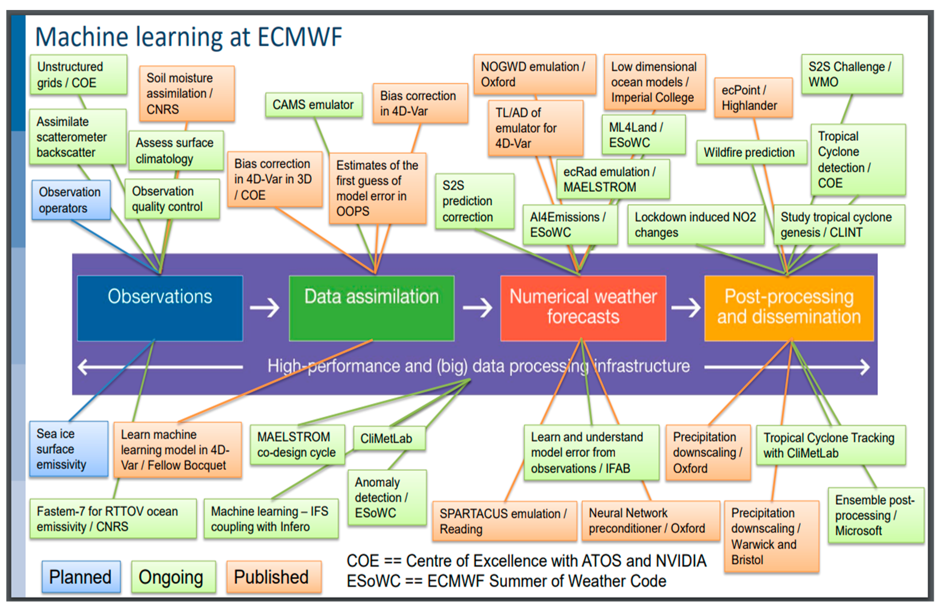
  40. Düben, P.; Modigliani, U.; Pappenberger, F.; Bauer, P.; Wedi, N.; Baousis, V. Machine Learning at ECMWF: A Roadmap for the Next 10 Years. ECMWF Tech. Memo. 2021, 878. Available online: https://www.ecmwf.int/sites/default/files/elibrary/2021/19877-machine-learning-ecmwf-roadmap-next-10-years.pdf (accessed on 20 March 2024).
  41. Krasnopolsky, V.M.; Fox-Rabinovitz, M.S. Complex Hybrid Models Combining Deterministic and Machine Learning Components for Numerical Climate Modeling and Weather Prediction. Neural Netw. 2006, 19, 122–134. [Google Scholar] [CrossRef]
  42. Brenowitz, N.D.; Bretherton, C.S. Prognostic Validation of a Neural Network Unified Physics Parameterization. Geophys. Res. Lett. 2018, 45, 6289–6298. [Google Scholar] [CrossRef]
  43. Dong, R.; Leng, H.; Zhao, J.; Song, J.; Liang, S. A Framework for Four-Dimensional Variational Data Assimilation Based on Machine Learning. Entropy 2022, 24, 264. [Google Scholar] [CrossRef] [PubMed]
  44. Bauer, P.; Geer, A.J.; Lopez, P.; Salmond, D. Direct 4D-Var assimilation of all-sky radiances. Part I: Implementation. Quat. J. R. Met. Soc. 2010, 136, 1868–1885. [Google Scholar] [CrossRef]
  45. Mellor, G.L.; Ezer, T. A Gulf Stream model and an altimetry assimilation scheme. JGR 1991, 96C, 8779–8795. [Google Scholar] [CrossRef]
  46. Guinehut, S.; Le Traon, P.Y.; Larnicol, G.; Philipps, S. Combining Argo and remote-sensing data to estimate the ocean three-dimensional temperature fields—A first approach based on simulated observations. J. Mar. Syst. 2004, 46, 85–98. [Google Scholar] [CrossRef]
  47. Krasnopolsky, V.; Nadiga, S.; Mehra, A.; Bayler, E. Adjusting Neural Network to a Particular Problem: Neural Network-based Empirical Biological Model for Chlorophyll Concentration in the Upper Ocean. Appl. Comput. Intell. Soft Comput. 2018, 2018, 7057363. [Google Scholar] [CrossRef]
  48. Cheng, S.; Chen, J.; Anastasiou, C. Generalized Latent Assimilation in Heterogeneous Reduced Spaces with Machine Learning Surrogate Models. J. Sci. Comput. 2023, 94, 11. [Google Scholar] [CrossRef]
  49. Hatfield, S.; Chantry, M.; Dueben, P.; Lopez, P.; Geer, T.; Palmer, A. Building Tangent-Linear and Adjoint Models for Data Assimilation with Neural Networks. J. Adv. Model. Earth Syst. 2021, 13, e2021MS002521. [Google Scholar] [CrossRef]
  50. Maulik, R.; Rao, V.; Wang, J.; Mengaldo, G.; Constantinescu, E.; Lusch, B.; Balaprakash, P.; Foster, I.; Kotamarthi, R. Efficient high-dimensional variational data assimilation with machine-learned reduced-order models. Geosci. Mod. Dev. 2022, 15, 3433–3445. [Google Scholar] [CrossRef]
  51. Krasnopolsky, V.M. Reducing Uncertainties in Neural Network Jacobians and Improving Accuracy of Neural Network Emulations with NN Ensemble Approaches. Neural Netw. 2007, 20, 454–461. [Google Scholar] [CrossRef]
  52. Geer, A.J.; Lonitz, K.; Weston, P.; Kazumori, M.; Zhu, Y.; Liu, E.H.; Collard, A.; Bell, W.; Migliorini, S.; Chambon, P.; et al. All-sky satellite data assimilation at operational weather forecasting centres. Quart. J. Roy. Meteor. Soc. 2017, 144, 1191–1217. [Google Scholar] [CrossRef]
  53. Krasnopolsky, V.M.; Fox-Rabinovitz, M.S.; Belochitski, A. Decadal climate simulations using accurate and fast neural network emulation of full, long- and short-wave, radiation. Mon. Weather Rev. 2008, 136, 3683–3695. [Google Scholar] [CrossRef]
  54. Krasnopolsky, V.M.; Fox-Rabinovitz, M.S.; Hou, Y.T.; Lord, S.J.; Belochitski, A.A. Accurate and Fast Neural Network Emulations of Model Radiation for the NCEP Coupled Climate Forecast System: Climate Simulations and Seasonal Predictions. Mon. Weather Rev. 2010, 138, 1822–1842. [Google Scholar] [CrossRef]
  55. Krasnopolsky, V.; Belochitski, A.; Hou, Y.-T.; Lord, S.; Yang, F. Accurate and Fast Neural Network Emulations of Long and Short Wave Radiation for the NCEP Global Forecast System Model. NCEP Off. Note 2012, 471. Available online: http://www.lib.ncep.noaa.gov/ncepofficenotes/files/on471.pdf (accessed on 20 March 2024).
  56. Pal, A.; Mahajan, S.; Norman, M.R. Using deep neural networks as cost-effective surrogate models for Super-Parameterized E3SM radiative transfer. Geophys. Res. Lett. 2019, 46, 6069–6079. [Google Scholar] [CrossRef]
  57. Roh, S.; Song, H.-J. Evaluation of neural network emulations for radiation parameterization in cloud resolving model. Geophys. Res. Lett. 2020, 47, e2020GL089444. [Google Scholar] [CrossRef]
  58. Ukkonen, P.; Pincus, R.; Hogan, R.J.; Nielsen, K.P.; Kaas, E. Accelerating radiation computations for dynamical models with targeted machine learning and code optimization. J. Adv. Model. Earth Syst. 2020, 12, e2020MS002226. [Google Scholar] [CrossRef]
  59. Lagerquist, R.; Turner, D.; Ebert-Uphoff, I.; Stewart, J.; Hagerty, V. Using deep learning to emulate and accelerate a radiative-transfer model. J. Atmos. Ocean. Technol. 2021, 38, 1673–1696. [Google Scholar] [CrossRef]
  60. Belochitski, A.; Krasnopolsky, V. Robustness of neural network emulations of radiative transfer parameterizations in a state-of-the-art general circulation model. Geosci. Model Dev. 2021, 14, 7425–7437. [Google Scholar] [CrossRef]
  61. Khain, A.; Rosenfeld, D.; Pokrovsky, A. Aerosol impact on the dynamics and microphysics of deep convective clouds. Q.J.R. Meteorol. Soc. A J. Atmos. Sci. Appl. Meteorol. Phys. Oceanogr. 2000, 131, 2639–2663. [Google Scholar] [CrossRef]
  62. Thompson, G.; Field, P.R.; Rasmussen, R.M.; Hall, W.D. Explicit Forecasts of Winter Precipitation Using an Improved Bulk Microphysics Scheme. Part II: Implementation of a New Snow Parameterization. Mon. Weather Rev. 2008, 138, 5095–5115. [Google Scholar] [CrossRef]
  63. Krasnopolsky, V.; Middlecoff, J.; Beck, J.; Geresdi, I.; Toth, Z. A Neural Network Emulator for Microphysics Schemes. In Proceedings of the AMS Annual Meeting, Seattle, WA, USA, 22–26 January 2017; Available online: https://ams.confex.com/ams/97Annual/webprogram/Paper310969.html (accessed on 20 March 2024).
  64. Jensen, A.; Weeks, C.; Xu, M.; Landolt, S.; Korolev, A.; Wolde, M.; DiVito, S. The prediction of supercooled large drops by a microphysics and a machine-learning model for the ICICLE field campaign. Weather Forecast. 2023, 38, 1107–1124. [Google Scholar] [CrossRef]
  65. Krasnopolsky, V.M.; Fox-Rabinovitz, M.S.; Belochitski, A.A. Using Ensemble of Neural Networks to Learn Stochastic Convection Parameterization for Climate and Numerical Weather Prediction Models from Data Simulated by Cloud Resolving Model. Adv. Artif. Neural Syst. 2013, 2013, 485913. [Google Scholar] [CrossRef]
  66. Schneider, T.; Lan, S.; Stuart, A.; Teixeira, J. Earth System Modeling 2.0: A Blueprint for Models That Learn from Observations and Targeted High-Resolution Simulations. Geophys. Res. Lett. 2017, 44, 396–417. [Google Scholar] [CrossRef]
  67. Gentine, P.; Pritchard, M.; Rasp, S.; Reinaudi, G.; Yacalis, G. Could Machine Learning Break the Convection Parameterization Deadlock? Geophys. Res. Lett. 2018, 45, 5742–5751. [Google Scholar] [CrossRef]
  68. Pal, A. Deep Learning Emulation of Subgrid-Scale Processes in Turbulent Shear Flows. Geophys. Res. Lett. 2020, 47, e2020GL087005. [Google Scholar] [CrossRef]
  69. Wang, L.-Y.; Tan, Z.-M. Deep Learning Parameterization of the Tropical Cyclone Boundary Layer. J. Adv. Model. Earth Syst. 2023, 15, e2022MS003034. [Google Scholar] [CrossRef]
  70. Krasnopolsky, V.M.; Lord, S.J.; Moorthi, S.; Spindler, T. How to Deal with Inhomogeneous Outputs and High Dimensionality of Neural Network Emulations of Model Physics in Numerical Climate and Weather Prediction Models. In Proceedings of the International Joint Conference on Neural Networks, Atlanta, GA, USA, 14–19 June 2009; pp. 1668–1673. Available online: https://ieeexplore.ieee.org/document/5178898 (accessed on 20 March 2024).
  71. Wang, X.; Han, Y.; Xue, W.; Yang, G.; Zhang, G.J. Stable climate simulations using a realistic general circulation model with neural network parameterizations for atmospheric moist physics and radiation processes. Geosci. Model Dev. 2022, 15, 3923–3940. [Google Scholar] [CrossRef]
  72. Scher, S. Toward data-driven weather and climate forecasting: Approximating a simple general circulation model with deep learning. Geophys. Res. Lett. 2018, 45, 616–622. [Google Scholar] [CrossRef]
  73. Scher, S.; Messori, G. Weather and climate forecasting with neural networks: Using GCMs with different complexity as study-ground. Geosci. Model Dev. Discuss. 2019, 12, 2797–2809. [Google Scholar] [CrossRef]
  74. Yik, W.; Silva, S.J.; Geiss, A.; Watson-Parris, D. Exploring Randomly Wired Neural Networks for Climate Model Emulation. arXiv 2022, arXiv:2212.03369v2. Available online: https://arxiv.org/pdf/2212.03369.pdf (accessed on 20 March 2024). [CrossRef]
  75. Pawar, S.; San, O. Equation-Free Surrogate Modeling of Geophysical Flows at the Intersection of Machine Learning and Data Assimilation. J. Adv. Model. Earth Syst. 2022, 14, e2022MS003170. [Google Scholar] [CrossRef]
  76. Schultz, M.G.; Betancourt, C.; Gong, B.; Kleinert, F.; Langguth, M.; Leufen, L.H.; Mozaffari, A.; Stadtler, S. Can deep learning beat numerical weather prediction? Philos. Trans. R. Soc. 2021, A 379, 20200097. [Google Scholar] [CrossRef]
  77. Wang, J.; Tabas, S.; Cui, L.; Du, J.; Fu, B.; Yang, F.; Levit, J.; Stajner, I.; Carley, J.; Tallapragada, V.; et al. Machine learning weather prediction model development for global ensemble forecasts at EMC. In Proceedings of the EGU24 AS5.5—Machine Learning and Other Novel Techniques in Atmospheric and Environmental Science: Application and Development, Vienna, Austria, 18 April 2024. [Google Scholar]
  78. Bi, K.; Xie, L.; Zhang, H.; Chen, X.; Gu, X.; Tian, Q. Accurate medium-range global weather forecasting with 3D neural networks. Nature 2023, 619, 533–538. [Google Scholar] [CrossRef] [PubMed]
  79. Kochkov, D.; Yuval, J.; Langmore, I.; Norgaard, P.; Smith, J.; Mooers, G.; Klower, M.; Lottes, J.; Rasp, S.; Duben, P.; et al. Neural general circulation models. arXiv 2023, arXiv:2311.07222. [Google Scholar]
  80. Xu, W.; Balaguru, K.; August, A.; Lalo, N.; Hodas, N.; DeMaria, M.; Judi, D. Deep Learning Experiments for Tropical Cyclone Intensity Forecasts. Weather. Forecast. 2021, 36, 1453–1470. [Google Scholar] [CrossRef]
  81. Krasnopolsky, V.M.; Fox-Rabinovitz, M.S.; Belochitski, A. Using neural network emulations of model physics in numerical model ensembles. In Proceedings of the 2008 IEEE International Joint Conference on Neural Networks, Hong Kong, China, 1–8 June 2008. 2008 IEEE World Congress on Computational Intelligence. [Google Scholar] [CrossRef]
  82. Kelpa, M.M.; Tessuma, C.W.; Marshall, J.D. Orders-of-magnitude speedup in atmospheric chemistry modeling through neural network-based emulation. arXiv 2018, arXiv:1808.03874. [Google Scholar]
  83. Schreck, J.S.; Becker, C.; Gagne, D.J.; Lawrence, K.; Wang, S.; Mouchel-Vallon, C.; Choi, J.; Hodzic, A. Neural network emulation of the formation of organic aerosols based on the explicit GECKO-A chemistry model. J. Adv. Model. Earth Syst. 2022, 14, e2021MS002974. [Google Scholar] [CrossRef]
  84. Sharma, H.; Shrivastava, M.; Singh, B. Physics informed deep neural network embedded in a chemical transport model for the Amazon rainforest. Clim. Atmos. Sci. 2023, 6, 28. [Google Scholar] [CrossRef]
  85. Geiss, A.; Ma, P.-L.; Singh, B.; Hardin, J.C. Emulating aerosol optics with randomly generated neural networks. Geosci. Model Dev. 2023, 16, 2355–2370. [Google Scholar] [CrossRef]
  86. Vannitsem, S.; Bjornar Bremnes, J.; Demaeyer, J.; Evans, G.R.; Flowerdew, J.; Hemru, S.; Lerch, S.; Roberts, N.; Theis, S.; Atencia, A.; et al. Statistical Postprocessing for Weather Forecasts: Review, Challenges, and Avenues in a Big Data World. BAMS 2021, 102, E681. [Google Scholar] [CrossRef]
  87. Klein, W.H.; Lewis, B.M.; Enger, I. Objective prediction of five-day mean temperatures during winter. J. Meteor. 1959, 16, 672–682. [Google Scholar] [CrossRef]
  88. Glahn, H.R.; Lowry, D.A. The use of model output statistics (MOS) in objective weather forecasting. J. Appl. Meteor. 1972, 11, 1203–1211. [Google Scholar] [CrossRef]
  89. Hemri, S.; Scheuerer, M.; Pappenberger, F.; Bogner, K.; Haiden, T. Trends in the predictive performance of raw ensemble weather forecasts. Geophys. Res. Lett. 2014, 41, 9197–9205. [Google Scholar] [CrossRef]
  90. Grönquist, P.; Yao, C.; Ben-Nun, T.; Dryden, N.; Dueben, P.; Li, S.; Hoefler, T. Deep learning for post-processing ensemble weather forecasts. Philos. Trans. R. Soc. 2021, A 379, 20200092. [Google Scholar] [CrossRef]
  91. Bouallègue, Z.B.; Cooper, F.; Chantry, M.; Düben, P.; Bechtold, P.; Sandu, I. Statistical Modelling of 2 m Temperature and 10 m Wind Speed Forecast Errors. Mon. Weather Rev. 2023, 151, 897–911. [Google Scholar] [CrossRef]
  92. Rojas-Campos, R.; Wittenbrink, M.; Nieters, P.; Schaffernicht, E.J.; Keller, J.D.; Pipa, G. Postprocessing of NWP Precipitation Forecasts Using Deep Learning. Weather Forecast. 2023, 38, 487–497. [Google Scholar] [CrossRef]
  93. Benáček, P.; Farda, A.; Štěpánek, P. Postprocessing of Ensemble Weather Forecast Using Decision Tree–Based Probabilistic Forecasting Methods. Weather Forecast. 2023, 38, 69–82. [Google Scholar] [CrossRef]
  94. Krasnopolsky, V.; Lin, Y. A Neural Network Nonlinear Multimodel Ensemble to Improve Precipitation Forecasts over Continental US. Adv. Meteorol. 2012, 2012, 649450. [Google Scholar] [CrossRef]
  95. Wang, T.; Zhang, Y.; Zhi, X.; Ji, Y. Multi-Model Ensemble Forecasts of Surface Air Temperatures in Henan Province Based on Machine Learning. Atmosphere 2023, 14, 520. [Google Scholar] [CrossRef]
  96. Acharya, N.; Hall, K. A machine learning approach for probabilistic multi-model ensemble predictions of Indian summer monsoon rainfall. MAUSAM 2023, 74, 421–428. Available online: https://mausamjournal.imd.gov.in/index.php/MAUSAM/article/view/5997 (accessed on 20 March 2024). [CrossRef]
  97. Rodrigues, E.R.; Oliveira, I.; Cunha, R.; Netto, M. DeepDownscale: A deep learning strategy for high-resolution weather forecast. In Proceedings of the 2018 IEEE 14th International Conference on e-Science (e-Science), Amsterdam, The Netherlands, 29 October–1 November 2018; pp. 415–422. [Google Scholar]
  98. Li, L. Geographically weighted machine learning and downscaling for high-resolution spatiotemporal estimations of wind speed. Remote Sens. 2019, 11, 1378. [Google Scholar] [CrossRef]
  99. Höhlein, K.; Kern, M.; Hewson, T.; Westermann, R. A comparative study of convolutional neural network models for wind field downscaling. Meteorol. Appl. 2020, 27, e1961. [Google Scholar] [CrossRef]
  100. Sekiyama, T.T. Statistical Downscaling of Temperature Distributions from the Synoptic Scale to the Mesoscale Using Deep Convolutional Neural Networks. arXiv 2020, arXiv:2007.10839. [Google Scholar]
  101. Sebbar, B.-E.; Khabba, S.; Merlin, O.; Simonneaux, V.; Hachimi, C.E.; Kharrou, M.H.; Chehbouni, A. Machine-Learning-Based Downscaling of Hourly ERA5-Land Air Temperature over Mountainous Regions. Atmosphere 2023, 14, 610. [Google Scholar] [CrossRef]
  102. Agrawal, S.; Carver, R.; Gazen, C.; Maddy, E.; Krasnopolsky, V.; Bromberg, C.; Ontiveros, Z.; Russell, T.; Hickey, J.; Boukabara, S. A Machine Learning Outlook: Post-processing of Global Medium-range Forecasts. arXiv 2023, arXiv:2303.16301. [Google Scholar] [CrossRef]
  103. Krasnopolsky, V.M.; Fox-Rabinovitz, M.S.; Tolman, H.L.; Belochitski, A. Neural network approach for robust and fast calculation of physical processes in numerical environmental models: Compound parameterization with a quality control of larger errors. Neural Netw. 2008, 21, 535–543. [Google Scholar] [CrossRef] [PubMed]
  104. Poggio, T.; Banburski, A.; Liao, Q. Theoretical issues in deep networks. Proc. Natl. Acad. Sci USA 2020, 117, 30039–30045. [Google Scholar] [CrossRef]
  105. Thompson, N.C.; Greenewald, K.; Lee, K.; Manso, G.F. The Computational Limits of Deep Learning. arXiv 2020, arXiv:2007.05558. [Google Scholar]
Figure 1. ML and various types of ML tools. There are many different types of NNs: shallow, deep, convolutional, recurrent, etc., as well as many types of tree algorithms. New ML tools emerge very often.
Climate 12 00078 g001
Figure 2. Some popular activation functions that are used in applications.
Climate 12 00078 g002
Figure 3. Relationships between ML, statistics, and mathematical theory [26,29].
Climate 12 00078 g003
Figure 4. Interdisciplinary complex climate and weather systems [15]. Only several major interactions (feedback) between major subsystems are shown with arrows.
Climate 12 00078 g004
Disclaimer/Publisher’s Note: The statements, opinions and data contained in all publications are solely those of the individual author(s) and contributor(s) and not of MDPI and/or the editor(s). MDPI and/or the editor(s) disclaim responsibility for any injury to people or property resulting from any ideas, methods, instructions or products referred to in the content.

