Abstract
The results of numerical experiments with a chemistry–climate model of the lower and middle atmosphere are presented to study the sensitivity of the polar stratosphere of the Northern and Southern Hemispheres to sea surface temperature (SST) variability, both as a result of interannual variability associated with the Southern Oscillation, and because of long-term increases in SST under global warming. An analysis of the results of model experiments showed that for both scenarios of SST changes, the response of the polar stratosphere for the Northern and Southern Hemispheres is very different. In the Arctic, during the El Niño phase, conditions are created for the polar vortex to become less stable, and in the Antarctic, on the contrary, for it to become more stable, which is expressed in a weakening of the zonal wind in the winter in the Arctic and its increase in the Antarctic, followed by a spring decrease in temperature and concentration of ozone in the Antarctic and their increase in the Arctic. Global warming creates a tendency for the polar vortex to weaken in winter in the Arctic and strengthen it in the Antarctic. As a result, in the Antarctic, the concentration of ozone in the polar stratosphere decreases both in winter (June–August) and, especially, in spring (September–November). Global warming may hinder ozone recovery which is expected as a result of the reduced emissions of ozone-depleting substances. The model results demonstrate the dominant influence of Brewer–Dobson circulation variability on temperature and ozone in the polar stratosphere compared with changes in wave activity, both with changes in SST in the Southern Oscillation and with increases in SST due to global warming.
1. Introduction
One of the consequences of global warming is an increase in sea surface temperature (SST) [1]. In turn, changes in SST affect air temperature, vertical temperature gradients that intensify vertical exchange, and consequently, atmospheric circulation [2]. At the same time, long-term climatic changes in SST are superimposed on interannual variations associated primarily with the El Niño–Southern Oscillation (ENSO) phenomenon. These and other SST variations lead to changes in heat and mass transfer between the atmosphere and the ocean, which affect surface air heating, vertical heat and mass fluxes, general atmospheric circulation, and consequently, weather, climate, and atmospheric chemistry not only in the lower atmosphere but also in the middle atmosphere both in the region of maximum SST variability and in regions remote from it [1,2]. Studying the features of the influence of SST variability on the temperature and gas composition of the lower and middle atmosphere at different latitudes offers great opportunities for a better understanding of the nuances of climate change against the background of short-term changes in the state of the atmosphere and ocean. At present, all of these problems are highly topical [1,2,3,4].
The manifestation of ENSO is that, in some years, the SST increases (El Niño) or decreases (La Niña) by a few degrees relative to the neutral phase in the tropical Pacific Ocean, creating the potential for rapid changes in ocean–atmosphere heat and mass transfer that affect the general circulation and wave activity in the atmosphere. Long-term changes in SST in recent decades are associated with overall global warming, part of which is an increase in SST by a few tenths of a degree from the early 1980s to the late 2010s across the globe [5], which also creates the potential for smooth changes in the general atmospheric circulation, temperature, and ozone in different regions of the Earth.
In addition to their direct influence on changes in the troposphere, SST variations due to vertical heat and mass fluxes also affect the structure, circulation, and composition of the stratosphere. The influence of SST variability on the stratosphere of polar regions is of particular interest because changes in the general atmospheric circulation can affect the stability of the stratospheric polar vortex (SPV) and wave activity at polar latitudes. In a stable SPV, the exchange of heat and mass between the polar and midlatitudes is limited, resulting in a decrease in the temperature within the polar vortex at stratospheric heights and a decrease in the ozone, whereas in an unstable SPV, the stratospheric temperature and ozone at midlatitudes and polar latitudes are leveled out [6,7,8].
Studies of the atmosphere–ocean interaction have a long history [6,7,8,9,10], with special attention paid to the influence of ENSO on changes in the temperature and gas composition of the atmosphere. In particular, it has been shown that sea warming during the El Niño phase leads to the weakening of the Walker circulation and trade winds, which creates the possibility of the feedback and influence of these changes on ENSO [5]. In [11], the importance of meridional transport in the tropics and zonal transport at the boundary of the Southern Oscillation region with the influence of Kelvin and Rossby waves was demonstrated.
The impact of SST on the dynamics and gas composition of the stratosphere, including the polar regions, has also been the subject of scientific research over the past few decades [12,13,14,15,16,17]. It has been shown [13,14] that changes in SST have a significant effect on the temperature and gas composition of the stratosphere in polar regions. It has also been shown [12] that zonal wind speed determines the stability of the SPV, with lower mean values of zonal wind in the Arctic than in the Antarctic and, on the contrary, greater interannual variations. A study of the variability in planetary waves revealed that the stability of the SPV is determined by the stability of the zonal transport of air masses, whereas an increase in the meridional transport leads to the instability of the SPV [16]. In addition, it was shown that planetary waves are one of the key factors affecting the existence of SPV in the Northern Hemisphere. The influence of meridional SST gradients on atmospheric circulation and ozone is shown in [15].
During the La Niña phase, as shown in [18], the weakening of the heat and mass flux into the stratosphere leads to the weakening of the BDC, the strengthening of zonal winds, an increase in the stability of the SPS, and a decrease in stratospheric air temperatures in the Arctic [18]. Simultaneously, as demonstrated in [19,20], the frequency of SSTs does not decrease during the La Niña phase, which may be related to the fact that during the La Niña phase, the North Pacific Ridge appears [21], which blocks the flows that could prevent the occurrence of SSTs.
The influence of ENSO on the polar stratospheric processes mainly occurs during the winter–spring period [22,23,24]. Typically, from November to mid-January, the SPV is stable during any ENSO phase, but in late winter, upward propagating planetary waves can weaken the SPV [25]. During the El Niño years, wave activity can increase in winter, and the amplitudes of planetary waves are most often higher than during the La Niña phase. As a consequence, waves propagate into the stratosphere, causing the weakening of the SPV in late winter and destruction of the SPV in spring [25,26,27].
Climate models are improving their ability to reproduce the phases of the Southern Oscillation and its influence on polar processes [28,29,30]. In particular, calculations carried out using an improved INM model showed that winter seasons with the El Niño phase are characterized by higher temperatures in the Arctic stratosphere than those with the La Niña phase [30]. Numerical estimations revealed that during the El Niño phase, the temperature in the Arctic stratosphere is 2 K higher, and the zonal wind speed is 5 m/s lower than that during the La Niña phase. An analysis of wave activity demonstrated that, in the winter months, planetary waves with zonal wave numbers 1 and 2 predominate with maximum amplitudes at 60–70 N latitude. In addition, it has been shown that during the El Niño phase, the amplitude of wave number 1 increases in the Arctic stratosphere, whereas during the La Niña phase, the amplitude of wave number 2 increases there [30].
Thus, previous studies have shown that an increase in SST during the El Niño ENSO phase, as well as a result of global warming, contributes to an increase in stratospheric heat flows and a weakening of the SPV, whereas the La Niña phase, corresponding to a SST decrease in the tropics, contributes to a weakening of the BDC and strengthening of the SPV. In addition, the weakening of the SPV may be associated with an increase in the flux of wave activity [31,32], while the strengthening of the SPV is associated with a weakening of the flux of wave activity. If the mechanisms of the influence of the strengthening or weakening of the SPV in the tropics on the BDC and through it on the SPV are generally clear, then their interaction with wave activity, as well as with changes in the SPV in other latitudes, still requires additional clarification.
In this study, as a follow-up to previous studies, both multiyear and interannual SST changes determining the interannual variability of atmospheric temperature and ozone are considered. Based on the analysis of the results of numerical experiments performed with the chemistry–climate model for different SST scenarios corresponding to different conditions of SST changes due to ENSO and long-term variability, the sensitivity of tropospheric and stratospheric temperature and ozone as a function of SST changes is evaluated. Section 2 describes the methodology, model, input data, and reanalysis data. Section 3 describes the analysis of SST changes, numerical experimental results, and reanalysis data for El Niño and La Niña scenarios and for the beginning and end of the 1980–2020 period. Section 4 provides a discussion. Section 5 summarizes the conclusions.
2. Materials and Methods
To analyze the sensitivity of atmospheric temperature and ozone to SST variability, numerical experiments with a chemistry–climate model (CCM) were performed, and the results were compared with reanalysis data.
For numerical experiments, we used the CCM developed at the Institute of Numerical Mathematics of the Russian Academy of Sciences and the Russian State Hydrometeorological University (INM RAS–RSHU CCM) [16,33,34,35]. The model consists of two parts: a dynamical part, which calculates meteorological variables and a chemical part, which calculates atmospheric gas parameters. The dynamical part of the model includes the basic equations of the hydrodynamics and thermodynamics of the atmosphere, which are solved by finite difference methods and are used to calculate the values of the main meteorological parameters. The resolution of the INM RAS–RSHU CCM is 4 × 5 latitude/longitude. The model grid is from 175° W to 180° E and from 88° S to 88° N. Vertically, the number of model σ levels is 39 (from the surface to the 0.003 hPa level, which approximately corresponds to the altitudinal interval from the surface to the mesopause). The number of grid points in the model is 72 in longitude and 45 in latitude. The exchange between the dynamical and chemical blocks is performed every 6 h (4 times a day).
The evolution of trace gasses is described using their transport equations, which are also solved using finite difference methods to determine the rates of chemical reactions. In addition to basic meteorological parameters, the CCM calculates the variability of 74 species of gasses in the lower and middle atmosphere for 174 chemical reactions in the gas phase and heterogeneous reactions, as well as 46 photolysis processes, including oxygen, nitrogen, hydrogen, chlorine, bromine, and hydrocarbon cycles [36,37,38]. The model includes processes of polar stratospheric cloud formation and evolution based on the distribution of sulfur aerosol in the stratosphere [37,38]. The dynamic of the polar vortex is calculated in the dynamical part of the CCM [38]. First, solar radiation fluxes are calculated by considering ozone concentration and molecular light scattering [37]. These fluxes are used to calculate the rates of the photodissociation of gasses, from which the rates of photochemical gas formation are calculated. In this case, the temperature values calculated in the dynamic part of the model are used for the calculation. Such rates of chemical reactions make it possible to simulate the evolution of ozone and other gasses [36].
The influence of SST and sea ice coverage (SIC) is considered in the dynamical part of the CCM as the lower boundary condition of the thermodynamic equation. The mean monthly SST and SIC data used from the Met Office reanalysis data [39] were interpolated to mean daily values and used to set the temperature at the lower boundary of the model at those points of the model grid that fall on the ocean.
In the first stage of the numerical experiments, the calculation with the CCM was performed for the climatic period from 1980 to 2020, in which the interannual variability of the factors influencing the temperature change and chemical composition was set: greenhouse gasses, sea surface temperature and its ice coverage area, atmospheric aerosol content, and the variability in solar activity fluxes. The results of the calculations were compared with the MERRA2 reanalysis and SBUV satellite data. Particular attention was paid to the variability in temperature and ozone in relation to the variability in ocean surface temperature in the tropical Pacific Ocean, both as a result of the long-period trend (trend) and interannual variations associated with ENSO phases. The purpose of these experiments was to determine the influence of SST variability against the background of the role of other factors and, first of all, the greenhouse gas content on the state of the lower and middle atmosphere.
In the second stage of the numerical experiments, calculations with the CCM were performed for several scenarios, in which we set repeated annual cycles of SST changes corresponding to each year from 1980 to 2020. Each scenario was calculated over 30 years. The results of the calculations for the last five years were averaged and, depending on the classification, assigned to one of four classes: the beginning of the climatic period with a neutral ENSO phase, the end of the climatic period with a neutral ENSO phase, the El Niño phase, and the La Niña phase. The purpose of this stage of numerical experiments was to isolate the influence of SST on temperature and ozone with other influencing factors unchanged. The calculations were performed from the beginning of 2020 with a repeating seasonal cycle for 2020 for all parameters except SST and SIC. Thus, the results of the calculations demonstrated the response of the lower and middle atmosphere temperature and ozone only to the changes in SST and SIC.
A criterion for SPV stability is the value of the zonal wind speed in the lower stratosphere at the boundary of the polar and middle latitudes. At large values of zonal wind, most of the warm and ozone-rich air from midlatitudes is carried away by the zonal flow around the polar region and does not penetrate the polar region. The increase in SST in the tropics during the El Niño phase of the Southern Oscillation can lead to the strengthening of the Brewer–Dobson circulation (BDC) because of which ozone and heat are transported from the tropical stratosphere toward the mid and polar latitudes, contributing to the increase in temperature and ozone there, while during the La Niña phase, on the contrary, the outflow of heat and ozone from tropical to mid and polar latitudes decreases. At the same time, the influence of the BDC on zonal wind and polar vortex stability is less obvious. On the one hand, an increase in the meridional flow can lead to a compensatory increase in the zonal flow, and on the other hand, the resulting increase in wave activity can lead to the inhibition of the zonal flow and weakening of the polar vortex stability [11,12,13]. The clarification of the ENSO influence on polar vortex stability is an interesting and timely task.
The results of the calculations for scenarios corresponding to the most powerful positive and negative SST anomalies in the tropical Pacific Ocean were particularly highlighted. These were 1983, 1998, and 2016, corresponding to the most powerful phase of El Niño, and 1989, 2000, and 2011, corresponding to the most powerful phase of La Niña [14,40,41,42]. For the analysis, differences in the mean values for the El Niño years and La Niña years for SST and atmospheric characteristics were calculated. Thus, the average calculated values of atmospheric parameters corresponding to the El Niño phase were compared with the average values corresponding to the La Niña phase. In addition, a similar comparison was conducted for years corresponding to the beginning of the climatic period and the neutral phase of ENSO (1981, 1982, and 1986), as well as the end of the climatic period and the neutral phase of ENSO (2014, 2017, and 2020) [5]. A comparison of the results of the calculations of the average values for these years at the beginning and end of the climatic period was used to analyze the influence of the SST trend on atmospheric parameters. The results of model calculations were compared with data from the Modern Age Retrospective Analysis for Research and Applications Version 2 (MERRA2 [43]) reanalysis for the period 1980–2020.
3. Results
3.1. Annual and Long-Term Changes in the SST
Figure 1a demonstrates the difference in SST between the three years with the most pronounced phases of El Niño and La Niña, according to the Met Office reanalysis. As expected, the maximum difference between the ENSO phases occurs in the tropical and subtropical Pacific. Moreover, if in the tropics (30S-30N) there is a significant increase of up to 4° in the El Niño phase compared to the La Niña phase, then in the subtropics, on the contrary, SST during the El Niño phase is up to 2° lower than during the La Niña phase. In addition, in the Atlantic and Indian Oceans, SST in the tropics during the El Niño phase is higher than that during the La Niña phase, whereas in the mid-latitudes, SST either changes little or decreases. This is especially pronounced in the Southern Hemisphere. Such temperature differences can influence both sea currents and SST changes in other regions and atmospheric circulation through changes in horizontal and vertical temperature gradients.
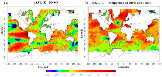
Figure 1.
Mean SST difference (degrees) between three years of El Niño (1983, 1998, and 2016) and three years of La Niña (1989, 2000, and 2011) (a) and between three years with neutral ENSO phase at the end of the climate period (2014, 2017, and 2020) and three years at the beginning of the period (1981, 1982, and 1986) from Met Office reanalysis data (b).
Figure 1b presents the Met Office SST differences at the end and beginning of the 1980–2020 climatic period. At the end of the period, the global average SST is 0.5–1.0° higher than that at the beginning of the period, most likely due to increased greenhouse gas emissions. The exception is the Pacific Ocean region near South America, where there has been a 1° decrease in SST, indicating ocean cooling in the ENSO region over the past 40 years. In addition, a decrease in SST toward the end of the period is observed near Antarctica. This decrease in SST may be due to the melting of Antarctic ice, which brings cold, fresh water into the ocean. In addition, a decrease in SST in some areas (especially in the tropics near Africa and Indonesia) may be associated with increased cyclonic activity and increased cloudiness and precipitation in these areas. At the same time, the maximum increase in SST is observed not in the tropics (30S-30N) but in the middle and polar latitudes of the Northern Hemisphere (Arctic amplification).
A comparison of SST anomalies for different phases of ENSO, as well as for the end and beginning of the climatic period 1980–2020, demonstrates that different changes in SST in different regions create the potential for changes in both horizontal and vertical air temperature gradients due to the influence of the underlying sea surface. This can affect heat and mass transfer between both neighboring regions and in the vertical direction. In addition, changes in regional circulation also affect the general circulation of the atmosphere, creating the possibility of long-term effects. In this work, special attention is paid to the atmospheric effects of SST variability, which, as can be seen from Figure 1a, are maximum in tropical and subtropical regions for years with El Niño and La Niña and in the polar and subpolar latitudes of the Northern Hemisphere for the end and beginning of the climatic period.
Before performing numerical experiments to assess the sensitivity of the atmosphere to SST variability, the model’s ability to reproduce atmospheric temperature variability during 1980–2020 was assessed. Figure 2 demonstrates the altitudinal variability of atmospheric temperature anomalies in comparison with average values for the period 1980–2020. Figure 2a,c presents the MERRA-2 reanalysis data for the tropics and the global scale, respectively, and Figure 2b,d presents similar results obtained as a result of the calculations using the INM RAS-RSHU CCM. The modeling results generally agree quite well with the reanalysis data both in the tropics and on a global scale. Both reanalysis data and CCM data show warming up to the tropopause (temperature increase by 0.5–1.0 degrees from 1980 to 2020 at altitudes up to 15–17 km) and stratospheric cooling (temperature decrease by 1.0–1.5 degrees above the tropopause). At the same time, ENSO-related (Table 1) temperature anomalies are present in the 0–20 km layer, which are more pronounced in the tropics (Figure 2a,c) but are also noticeable on a global scale (Figure 2b,d). It can be seen that both positive atmospheric temperature anomalies associated with the El Niño phase and its negative anomalies associated with the La Niña phase are more pronounced not near the surface, where heat exchange with the sea occurs but at altitudes of approximately 10 km. This effect is noticeable not only in the tropics, where it can be explained by developed convective movements, but also in extratropical latitudes, which once again emphasizes the role of circulation processes affecting teleconnection in the atmosphere.

Figure 2.
Atmospheric temperature anomalies (in degrees) in the troposphere and stratosphere of the tropics (30S-30N) from the MERRA-2 reanalysis (a) and numerical experiments with CCM INM RAS-RSHU (b) and on a global scale from the MERRA-2 reanalysis (c) and numerical experiments with CCM INM RAS-RSHU (d).

Table 1.
ENSO phases and SST anomalies at 170–120 W (Niño 3.4 region). A more detailed table is presented in [42].
Figure 3 presents the variability in stratospheric ozone during 1980–2020 in the Antarctic and Arctic according to the SBUV satellite measurements and the results of numerical modeling with the INM RAS-RSHU CCM. The results of satellite measurements and numerical modeling qualitatively correspond well to each other, although there are also quantitative discrepancies. Both in the Antarctic and Arctic, the model reproduced the values observed by satellite instruments in the 1990s, with minimum ozone values in the Antarctic in the second half of the 1990s and in the Arctic in the first half of the 1990s. In the early 2000s, the model also reproduced the observed alternations of the periods of ozone increase and decrease quite well, but after 2015, the results of satellite observations and numerical modeling diverged significantly. The influence of the Southern Oscillation in the polar stratosphere is manifested, as a rule, in the next year because the maximum changes in SST corresponding to different phases of the Southern Oscillation occur in the second half of the year [42], preceding the winter–spring period in the Arctic. In the Antarctic, the change in the SST most often occurs after the polar night and does not have time to influence the formation of the polar vortex and can only partially influence its destruction in the process of the final warming or it could manifest itself next year.

Figure 3.
Atmospheric ozone anomalies in the troposphere and stratosphere of the Antarctic from the SBUV (a) and numerical experiments with CCM INM RAS-RSHU (b) and on Arctic from the SBUV (c) and numerical experiments with CCM INM RAS-RSHU (d).
Ozone depletion in the Arctic stratosphere is observed and reproduced by the model after the La Niña phase (Table 1) in 1983, 1986, 1997, 2000, and 2011. At the same time, the minima in the early 1990s, 2016, and 2020, are not related to the preceding Southern Oscillation phase but are determined by other causes. The model reproduces the minimum in the early 1990s, but in 2016 and 2020, only a slight decrease in ozone is simulated, without reproducing a significant ozone depletion. After the El Niño phase, significant increases in Arctic stratospheric ozone are recorded by satellite observations and reproduced by the model in 1981, 1984, 1987, 1988, 1999, 2004, 2006, 2010, 2015, and 2019. In Antarctica, ozone maxima are recorded the year after El Niño in 1981, 1988, 2004, and 2016 and minima after the preceding La Niña phase in 2001, 2007, and 2019. At the same time, the Antarctic minima throughout the 1990s, when significant positive and negative SST anomalies alternated, are probably not directly connected with the phases of the Southern Oscillation and are more likely determined by other factors, in particular, volcanic emissions and solar activity.
A comparison of the results of numerical modeling with the data of satellite measurements and reanalysis demonstrated that the phases of the Southern Oscillation do not always definitely define the stability of the polar vortex, stratospheric cooling, and ozone variations inside it. Other factors also play an important role. In order to separate the influence of other factors and to determine the sensitivity of polar processes only to the variability in SST, numerical experiments were further carried out in which only SST was varied and other factors did not change from year to year.
To analyze the sensitivity of atmospheric parameters to short- and long-term changes in SST, the following sections present the CCM-calculated changes in temperature, ozone, and dynamic parameters affecting heat and mass transfer and the polar vortex. As is known, ENSO leads to an increase in air temperature in the troposphere [5,19,22,28]. As a result, atmospheric heat flow is stronger in the equatorial Pacific and over the Arctic and weaker over Antarctica. This may indicate a deepening of the Aleutian Low in the Northern Hemisphere due to El Niño, as well as an increase in heat flow into the Arctic stratosphere. The warming of the troposphere during El Niño leads to increased temperature contrasts between the tropics and polar latitudes, which contributes to increased cyclonic activity in the mid-latitude Pacific Ocean. Heat captured by cyclones in the upper troposphere can penetrate into the lower stratosphere and contribute to SSW [5,19,23,26,27,28].
3.2. Impact of ENSO on Stratospheric Processes
This chapter presents the results of numerical experiments in which the INM RAS-RSHU CCM was run starting from 2021 for 10 years with a repeating annual cycle of influencing factors. A total of 41 model runs were performed, each of which used SST data for every year from 1980 to 2020. Other factors (solar activity, changes in the gas composition of the atmosphere due to emissions and absorption, etc.) were fixed at the 2020 level. A comparison of the calculation results made it possible to assess the sensitivity of atmospheric chemistry and climate parameters only to interannual SST variability, with other influencing factors remaining unchanged from year to year.
In the first stage, from an ensemble of 41 model runs based on Table 1 [42], years with El Niño and La Niña were selected, and the average zonal mean vertical profiles of the anomalies in air temperatures, ozone, and zonal wind were calculated for them (Figure 4). As can be seen, throughout the year over the tropical region, there is an increase in temperature of more than 0.5° for El Niño (Figure 4b) and a decrease of 0.2–0.5 degrees for La Niña (Figure 4a) at altitudes of the upper troposphere–lower stratosphere, then from winter to autumn in the middle stratosphere a decrease to 0.2 degrees. In autumn, when the Southern Oscillation begins to manifest itself most intensely [42], the maximum increase in temperature in the tropics is observed at altitudes from 20 to 30 km. In polar latitudes (60–90 degrees) in September–November, cooling is observed in the lower stratosphere, and in Antarctica, it is more significant than in the Arctic in La Niña. During the winter months in the Arctic, there is an increase in temperature by 1–2 degrees at altitudes of 10–40 km and a decrease in temperature by more than 2° at altitudes of 50–60 km in El Niño. In Antarctica, in winter (June–August), the stratosphere temperature is also higher in the El Niño years than in the La Niña years and lower in the spring months.
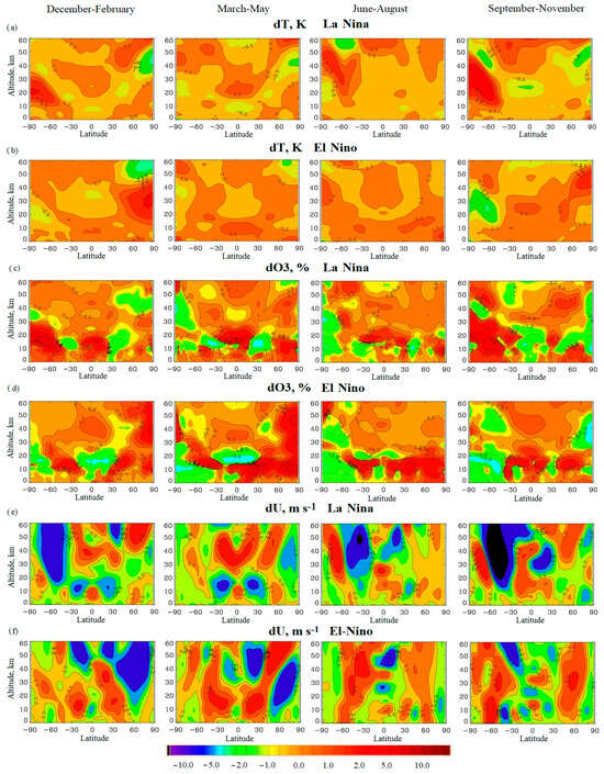
Figure 4.
Vertical zonal mean profiles of anomalies in air temperature for scenarios with El Niño and La Niña phases (a,b), ozone concentration for scenarios with El Niño and La Niña phases (c,d), and zonal wind speed in m/s for scenarios with El Niño and La Niña phases (e,f) based on modeling results.
Figure 4c,d presents the vertical profiles of anomalies in ozone concentrations based on simulation results for the La Niña and El Niño scenarios. In the winter–spring period of the Northern Hemisphere (December–May) in El Niño, a decrease in ozone is observed in the tropics, and in the Arctic during the same period, ozone increases. In La Niña, ozone in the tropics increases and decreases in 30–60 N. In the winter–spring period of the Southern Hemisphere (June–November), on the contrary, in the tropical stratosphere, ozone increases, and in the Antarctic stratosphere, it decreases, especially in the spring, i.e., the ozone hole is getting deeper. In La Niña, ozone in Southern Hemisphere increases in autumn and winter and decreases in spring and summer. For the zonal wind (Figure 4e,f), it can be noted that at the border of the polar region in winter, the zonal speed in the Arctic (December–February) in the El Niño years is significantly lower than in the La Niño years, while in the Antarctic winter (June–August), the zonal speed at the polar boundary increases during the El Niño years. This means that in the Arctic, the polar vortex becomes less stable during the El Niño phase, and in the Antarctic, it becomes more stable.
Changes in ozone and temperature in the polar stratosphere can be associated with both the strengthening or weakening of the BDC and changes in wave activity at the boundary of the polar regions. Therefore, we consider changes in the residual circulation in the stratosphere coinciding with the BDC and the amplitudes of atmospheric waves with wave numbers 1 and 2. Figure 5 presents vertical profiles of the anomalies between the meridional (Figure 5a,b) and vertical (Figure 5c,d) components of the residual circulation, based on the simulation results for scenarios with the La Niña and El Niña phases. In the winter months of the Northern Hemisphere (December–February), in the El Niño phase throughout the stratosphere, there is an increase in meridional transport from the middle latitudes to the Arctic, accompanied by a weakening of the vertical transport (Figure 5d) and zonal wind (Figure 4f), i.e., the polar vortex is weakened. In La Niña, meridional transport from the middle latitudes to the Arctic decreases, and zonal wind (polar vortex) intensifies.
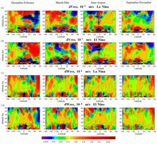
Figure 5.
Seasonal profiles of the anomalies between the meridional (a,b) and vertical (c,d) components of the residual circulation based on the modeling results for the scenarios with La Niña and El Niño phases.
In the Southern Hemisphere, where the strengthening of the meridional transport toward the pole corresponds to negative differences, during the winter period (June–August), the meridional transport toward the pole increases in the middle latitudes, just up to the border with the polar region, and in the polar region, this flow is slowed down or even turns away from the pole. The result of this is an increase in the vertical rise inside the polar region, with its weakening just beyond its border (Figure 5c,d), and an increase in the zonal wind (Figure 4e,f), i.e., the polar vortex is intensifying.
The change in the amplitudes of atmospheric waves at the polar boundary characterizes the change in their impact on the polar vortex; therefore, Figure 6 demonstrates the changes in the amplitudes of waves with wave numbers 1 and 2 in the experiments with SST corresponding to the El Niño phase and experiments with SST with the La Niña phase compared to the average values. For wave number 1 in El Niño (Figure 6b), an increase in amplitude is observed in both the Northern Hemisphere (December–February) and Southern Hemisphere (March–August) during the winter period. However, in the Northern Hemisphere, the amplitude of wave number 1 increases more strongly, especially in the lower stratosphere. Simultaneously, in the spring period, when the polar vortex is finally destroyed due to the final warming, the amplitude of wave number 1 decreases in the Northern Hemisphere, while in the Southern Hemisphere, it increases at the polar boundary. In La Niña (Figure 6a), the amplitude of wave number 1 decreases in both hemispheres, but in the Southern Hemisphere, the amplitude increases in 30–60 altitudes. For wave number 2 (Figure 6c,d), in El Niño, the amplitude decreases in the Northern Hemisphere in winter and spring at the polar boundary, whereas in the Southern Hemisphere, it increases in winter and decreases in spring. In La Niña, this amplitude in the Northern Hemisphere increases in winter and summer, decreases in 10–30 km and increases in 30–60 km in spring, and decreases in autumn. In the Southern Hemisphere, this amplitude increases but decreases in summer. Thus, it can be stated that with the change in phases of the Southern Oscillation, wave number 1 contributes more to the destruction of the polar vortex during the El Niño phase than during the La Niña phase in the Northern Hemisphere, and wave number 2 contributes more in the Southern Hemisphere than in the Northern Hemisphere.
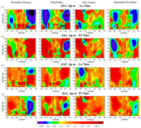
Figure 6.
Zonally mean seasonally averaged profiles of the differences between the wave amplitude with wave number 1 (a,b) and the wave amplitude with wave number 2 (c,d) from modeling results for scenarios with La Niña and El Niño phases.
In general, for the combined influence of BDC variability and wave activity on polar processes when the phase of the Southern Oscillation changes from La Niña to El Niño, the influence of BDC variability can be noted. In particular, in the Northern Hemisphere in winter, at the boundary of the polar region, the BDC and wave 1 intensify and wave 2 weakens. At the same time, despite the compensation of wave numbers 1 and 2, due to the strengthening of the BDC, the zonal wind at the boundary of the polar region weakens, the stability of the polar vortex decreases, and the temperature and ozone increase (Figure 4). At the same time, because the vortex during the winter during El Niño becomes less stable, the spring destruction of ozone decreases and its content increases not only in winter but also in spring, although in the spring, dynamical conditions do not contribute to the accumulation of ozone in the Arctic. In Antarctica, both wave 1 and wave 2 intensify during the transition from the La Niña phase to the El Niño phase, which creates the potential for a weakening of the polar vortex. However, wave 2 intensifies in winter and spring, which is associated with the weakening of the BDC at the boundary of the polar region. As a result, during the spring period of the Southern Hemisphere (September–November), both temperature and ozone decreased in the lower stratosphere of Antarctica (Figure 4).
This conclusion is supported by the figures in Appendix A for changes in temperature and ozone at an altitude of 100 hPa (Figure A1) and the flux of Plumb wave activity (Figure A2). Figure A1 presents a decrease in ozone concentration in the tropical stratosphere, especially over the equatorial Pacific, whereas over the Arctic, there is an increase in ozone concentration of 3–5% and a decrease of 3–4% over Antarctica. Total ozone (Figure A1b) demonstrates a 1–2% decrease in ozone concentrations in the tropics, especially over the Pacific Ocean in the El Niño region, consistent with air temperature (Figure 4c) and ozone concentration in the lower stratosphere, and indicates an increase in the Brewer–Dobson circulation in the tropics during the El Niño years. A decrease of 0.5–1% is also observed over Greenland and Antarctica, while over the Arctic, during El Niño years, an increase of 2% is observed compared with the La Niña phase. Over Antarctica, there is a 3% decrease in ozone compared with the La Niña phase. There is also a 0.5% increase in ozone between Australia and Antarctica. This indicates an increase in the Brewer–Dobson circulation during the El Niño years, which contributes to the increased transport of ozone from the tropics to the polar regions and, as a result, an increase in ozone over the Arctic and a decrease in ozone in the tropics, from where it is carried to the poles. The El Niño effect in Antarctica is weaker than that in the Arctic.
As for stratospheric air temperature (Figure A1c), over the equatorial Pacific Ocean, there is a decrease in air temperature by 2.5°, while south of the equatorial Pacific Ocean and in most of the Arctic, the temperature rises by 1.8–2 degrees. These features may be associated with increased stratospheric heat flow due to the El Niño event, which contributes to increased stratospheric heat flow and SPV [28] and indicates a warming of the Arctic stratosphere and an increase in the probability of SSW, which affects the zonal wind [28] and contributes to SPV instability and an intensification of the Brewer–Dobson circulation, promoting the transfer of heat and ozone from the tropical stratosphere to the polar stratosphere. A decrease in temperature by 1–2 degrees is also observed over the Antarctic south of Australia, which may be due to the blocking of the polar region by meridional circulation for most of the year, starting in spring, the intensification of the zonal wind at its boundary, and the cooling of the lower polar stratosphere (Figure 4). An increase of 0.2 degrees is observed over the outskirts of South America, which indicates weak stratospheric warming in the Southern Hemisphere and contributes to a slight weakening of the temperature and SPV stability and an increase in total ozone.
Figure A1 presents a decrease in ozone concentration in the tropical part of the stratosphere, especially over the equatorial part of the Pacific Ocean, while an increase in ozone concentration by 3–5% is seen over the Arctic and a decrease of 3–4% over the Antarctic. The total column ozone (Figure A1b) shows a 1–2% decrease in the tropics, especially over the Pacific Ocean in the El Niño region, which is consistent with air temperature (Figure A1c) and ozone concentration in the lower stratosphere, and indicates a strengthening of the Brewer–Dobson circulation in the tropics during the El Niño years. A decrease of 0.5–1% is also observed over Greenland and Antarctica, while over the Arctic, there is an increase of 2% in the El Niño years compared to the La Niña phase. Over Antarctica, there is a decrease in ozone by 3% compared with the La Niña phase. In addition, a 0.5% increase in ozone is observed between Australia and Antarctica. This indicates the strengthening of the Brewer–Dobson circulation during the El Niño years, which contributes to the increased transport of ozone from the tropics to the polar regions and, as a result, to the increase in ozone over the Arctic and the decrease in ozone in the tropics, from where it is carried to the poles. The El Niño effect is weaker in the Antarctic than in Arctic.
Regarding stratospheric air temperature (Figure A1c), a 2.5° decrease in air temperature is observed over the equatorial Pacific Ocean, whereas south of the equatorial Pacific and over much of the Arctic, the temperature increases by 1.8–2 degrees. These features may be related to enhanced stratospheric heat flux due to El Niño phenomena, which contribute to an enhanced stratospheric heat flux and SSW [28], and indicate the heating of the Arctic stratosphere and increased probability of SSW, which affects the zonal wind [28] and contributes to the instability of the SPV and enhanced Brewer–Dobson circulation, contributing to the transfer of heat and ozone from the tropical stratosphere to the polar stratosphere. A temperature decreases by 1–2 degrees is also observed over the Antarctic south of Australia, while over the vicinity of South America, there is an increase by 0.2°, indicating weak stratospheric warming in the Southern Hemisphere and contributing to a slight weakening of the SPV and an increase in total ozone.
An analysis of the variability in the components of the Plumb wave activity flow during changes in the phases of the Southern Oscillation allows us to estimate the variability in wave activity because of the total influence of waves with all wave numbers. An analysis of the change in the Plumb flow with SST changes from La Niña to El Niño (Figure A2, zonal component (a), meridional component (b) and vertical component (c)) demonstrates that over the Northern Hemisphere, there is a strong increase in the zonal component of the Plumb flow at altitudes of 30–60 km by 10 m2s−2 and the vertical component of the Plumb flow by 2–5 × 10⁻² m2s−2 at altitudes of 20–60 km in the winter and autumn months. The meridional component decreased 10 m2 s−2 at altitudes 30–60 and exhibited an enhancement of 0.5 m2 s−2 at altitudes 10–30 km. At altitudes of 0–30 km and 30–60 latitudes in the winter months, a decrease in flow by 0.5 m2 s−2 is observed. The strengthening of the meridional and vertical components at the altitudes of 20–30 km is related to the strengthening of meridional processes due to stratospheric heating, which contribute to the weakening of the zonal flux and Rossby waves. This amplification indicates an increase in the intensity of propagation of planetary Rossby waves from the troposphere to the stratosphere due to enhanced heat fluxes from the stratosphere during the Southern Oscillation. These heat fluxes contribute to the enhanced wave activity flux from the tropics to the pole and from the troposphere to the stratosphere, which contributes to the instability of Rossby waves. All of this affects the zonal wind and disrupts the SPV, resulting in enhanced Brewer–Dobson circulation and heat and ozone transport from the tropics to the polar regions. As for the Southern Hemisphere, at the altitudes of 40–60 km, one observes an intensification of the zonal component of the Plumb flux in the spring and autumn months by 0.5 m2 s−2. In the summer months, an increase of 5 m2 s−2 is observed at altitudes 0–30 km. The meridional component shows an increase by 0.5 m2 s−2 in the spring and fall months and by 5 m2 s−2 in the summer months at altitudes of 20–50 km, indicating an increase in the meridional flux of wave activity from the equator to the South Pole. The vertical component shows an increase of 0.5 × 10⁻² m2 s−2 during the spring and fall months at altitudes of 20–60 km and 2 × 10⁻² m2 s−2 during the summer months at altitudes of 30–60 km. These phenomena indicate the strengthening of the wave activity flux in the Northern Hemisphere and weakening of this flux in the Southern Hemisphere, which, in turn, contributes to the weakening of planetary Rossby waves and the destruction of the SPV, especially in the Northern Hemisphere, and the transfer of heat by planetary waves from the equator to the pole and from the troposphere to the stratosphere. Correlation coefficients between the ENSO phases and wave activity flux are, on average, 0.8–0.9 in the Northern Hemisphere and 0.7–0.8 in the Southern Hemisphere.
The divergence of the wave activity flow shows the total effect of all components of the Plumb vector when the phases of the Southern Oscillation change (Figure A2d). There is a negative anomaly between El Niño and La Niña phases in the Northern Hemisphere at 30–60 km altitudes in the winter and fall months of 2–5 s−2 and weaker (up to 0.5 s−2) in the spring months. In the Southern Hemisphere, there is a weak negative divergence anomaly in the spring and summer months (up to 2 s−2) at altitudes of 40–60 km. This means that during the El Niño phase, there are more dramatic changes in the flow of wave activity in the Northern Hemisphere than during the La Niña phase. El Niño contributes to the enhancement of the meridional and vertical flux of wave activity into the stratosphere. This contributes to the enhanced convergence of the Plumb flow, as indicated by the negative anomalies, and hence to the reversal of the zonal flow and weakening of the Rossby waves. These changes are related to the enhanced heat flux into the stratosphere during the El Niño phase, which contributes to the enhanced meridional temperature transport from the tropics to the polar regions, which affects the zonal wind, and contributes to the enhanced wave activity flux. This both weakens the planetary Rossby waves during the El Niño phase and enhances the propagation of heat into the stratosphere through these waves, which contributes to the destruction of the SPV and SSW. In the Southern Hemisphere, this influence is much weaker than in the Northern Hemisphere. In general, the analysis of the divergence of the wave activity flux demonstrates its insignificant variability in the lower stratosphere, which confirms the predominance of the influence of the BDC on the polar stratosphere compared to wave activity when the phases of the Southern Oscillation change.
3.3. Influence of the Long-Term SST Variability on Stratospheric Processes
In addition to analyzing the impact of short-term interannual variability associated with ENSO, an analysis of the simulation results sampled for the neutral phase of ENSO in the late 2010s was performed in relation to the results of the numerical experiments corresponding to the neutral phase of the early 1980s. Simultaneously, as in the case of ENSO, the remaining factors were fixed at the 2020 level, which made it possible to analyze only the results of the influence of long-term SST variability on the structure and composition of the atmosphere.
Figure 7a presents vertical profiles of the air temperature difference between the modeling results for the SST corresponding to the end and beginning of the 40-year period. The troposphere exhibits almost uniform warming throughout the year, highlighting the impact of SST variability on global warming. In the stratosphere, the most significant temperature changes occur in the polar regions. At the same time, cooling is observed in the Antarctic polar stratosphere during the entire year, with the maximum effect in the winter–spring period of the Southern Hemisphere (June–November), which creates the potential for intensifying the processes of the formation of polar stratospheric clouds and heterogeneous processes on their surface, contributing to the increased spring destruction of ozone and deepening of ozone holes. In the Arctic polar stratosphere, winter temperatures vary little compared to the warmer mid-latitude lower stratosphere, creating a temperature gradient and potential for poleward meridional flow. In the spring, in the lower stratosphere of the Arctic, on the contrary, the temperature increase is greater than that in the middle latitudes, which contributes to a more rapid destruction of polar stratospheric clouds if they were able to form in winter.
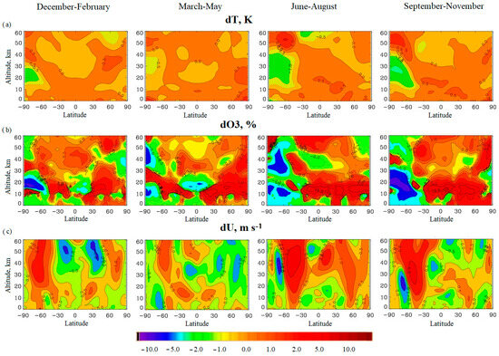
Figure 7.
Vertical zonal mean seasonal profiles of air temperature differences (a), ozone concentration (b), and zonal wind speed in m/s (c) based on modeling results for the scenarios of the early 1980s and late 2010s.
Figure 7b presents the vertical profiles of the differences in ozone concentrations between the simulation results at the end and beginning of the review period. In the tropics, ozone concentration in the upper troposphere–lower stratosphere decreases in the winter–spring period of the Northern Hemisphere (December–May) and increases in the winter–spring period of the Southern Hemisphere (June–August). At the same time, in the Arctic stratosphere in winter, ozone increases in the lower part and increases in the upper part.
This corresponds to an increase in zonal velocity at the polar boundary in the middle and upper stratosphere (Figure 7c). This means that the polar vortex becomes more stable in the Arctic in winter only in the upper part of the stratosphere, with a long-term increase in sea temperature, whereas in the lower part, it becomes less stable. In Antarctica, the ozone concentration in the polar stratosphere decreases both in winter (June–August) and in spring (September–November). This is a result of global warming, and the zonal flow at the boundary of the south polar region increases in both winter and spring (Figure 7c). As a result, the Antarctic polar vortex becomes more stable, leading to a cooling trend in the lower stratosphere (Figure 7a) and a decrease in ozone (Figure 7b,c) during the winter–spring period. Thus, global warming associated with a positive SST trend creates conditions for the deepening of the Antarctic ozone hole in contrast to the tendency for ozone recovery because of the reduced emissions of ozone-depleting substances. The correlation coefficients between the SST trend and zonal wind speed anomalies are 0.7–0.8 in the Northern Hemisphere and 0.8 in the Southern Hemisphere.
To clarify the role of changes in the BDC and wave activity in the influence of global warming on changes in temperature and ozone, we further consider the variability in the components of the residual circulation and the amplitudes of planetary waves for the beginning and end of the climatic period 1980–2020. Figure 8 demonstrates the variability in the meridional (Figure 8a) and vertical (Figure 8b) components of the residual circulation at the end of the 2010s relative to the beginning of the 1980s. In the Northern Hemisphere, the meridional flow toward the pole at the boundary of the polar region in the lower stratosphere increases in winter and spring, as a result of which the vertical speed also increases (Figure 8b), and the zonal wind increases only in the upper stratosphere (Figure 7c). As a result, ozone is reduced in the middle and upper stratosphere of the Arctic (Figure 7b). At the Antarctic border, the meridional flow toward the pole weakens during the winter–spring period (June–November), and the vertical velocity increases inside the polar region and weakens in the middle latitudes near the border with the polar region. This leads to the fact that the polar vortex strengthens (an increase in the zonal velocity at the boundary of the polar region—Figure 7c), and for temperature (Figure 7a) and ozone (Figure 7b), a tendency to decrease is formed.
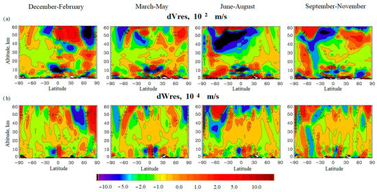
Figure 8.
Differences between the meridional (a) and vertical (b) components of the residual circulation based on the modeling results for the scenarios of the late 2010s and early 1980s.
To analyze the impact of global warming on wave activity, Figure 9 shows the differences in the amplitudes of planetary waves with wave number 1 (Figure 9a) and wave number 2 (Figure 9b) based on the results of experiments for the end and beginning of the climate period 1980–2020. The amplitude of wave 1 in the Arctic and subarctic regions greatly decreases in winter, whereas wave 2 increases significantly during the same period. These effects are exactly opposite to those observed for ENSO (Figure 6). However, changes in wave activity, as well as for ENSO, do not have a fundamental effect on changes in ozone and temperature. Thus, a decrease in the amplitude of wave 1 in the Arctic in winter should strengthen the polar vortex and lead to a decrease in temperature and ozone. This effect can only be noted for ozone in winter in the upper stratosphere (Figure 7b), and the temperature, on the contrary, increases. Changes in wave activity affect temperature and ozone levels in Antarctica even less. In the summer–spring period, a significant increase in the amplitude of wave 1 and a slight decrease in wave 2 are recorded there. Theoretically, such a change in wave activity should have led to a weakening of the polar vortex, warming, and an increase in ozone concentration. However, the results of the numerical experiments show cooling in the Antarctic stratosphere (Figure 7a) and a decrease in ozone (Figure 7b), with an intensifying polar vortex (Figure 7c). This, as with ENSO, demonstrates the dominant influence of Brewer–Dobson circulation variability (Figure 8) compared with changes in wave activity (Figure 9).
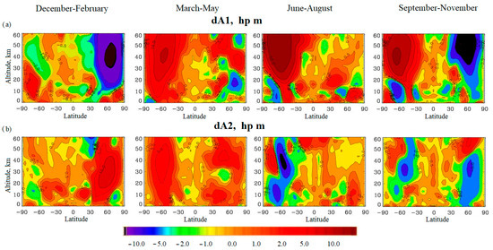
Figure 9.
Vertical zonal mean seasonal profiles of the differences between wave amplitude with wave number 1 (a) and wave amplitude with wave number 2 (b) from modeling results for the late 2010s and early 1980s scenarios.
Appendix A presents maps of the distribution of air temperature differences, ozone concentrations, and total ozone in the lower stratosphere as a result of global warming (Figure A3). These figures show an increase in ozone concentration and total ozone of 1–3% over the tropical Pacific and 0.5% in the Arctic stratosphere and a decrease of 3–5% in the Antarctic stratosphere. We also see a 1–3% decrease in ozone and total ozone over the tropical Atlantic and over Siberia. The distribution of differences in ozone corresponds to the temperature of the stratospheric air (Figure A3c). The decrease in ozone concentration and total column ozone is observed mainly in the Southern Hemisphere over the Atlantic. In the Northern Hemisphere, ozone levels are increasing, with the exception of Siberia. The decrease in ozone in the tropics and the increase in the Northern Hemisphere indicate an increase in the Brewer–Dobson circulation, which transports air temperature and ozone from the tropics to the poles, but this effect is much smaller than in the case of ENSO. In the Southern Hemisphere, there is practically no transfer of ozone to the Southern Hemisphere, which is why the ozone decreases.
As for the air temperature in the stratosphere (Figure A3c), a warming of 1–2 degrees are observed over the tropics, especially over the Pacific Ocean and Australia, and by 1 degree over the Canadian Arctic. Also, in the stratosphere, there is a decrease in temperature in the Southern Hemisphere by 0.5–1.0 degrees, and over the Arctic in the region of Chukotka and Alaska—by 1–2 degrees. The increase in temperature over the Atlantic and North America is due to increased heat fluxes from the troposphere and SSW. SST changes have a much smaller impact on the stratosphere than on the troposphere, but nevertheless, the ocean still affects it indirectly. Compared to ENSO, the influence of the SST trend on the stratosphere is less significant. However, an increase in SST still contributes to increased heat fluxes in the stratosphere, as evidenced by rising air temperatures in the Northern Hemisphere. In the Southern Hemisphere, air temperatures are decreasing, indicating a weakening of heat fluxes in the stratosphere over Antarctica and an increase in zonal fluxes.
Figure A4 presents the vertical flow of wave activity. Vertical profiles of the differences between the zonal (Figure A4a), meridional (Figure A4b), and vertical (Figure A4c) components and the divergence (Figure A4d) flux of wave activity between the simulation results for the trend end and trend start scenarios are presented below. As can be seen, over the Arctic at altitudes of 20–50 km in the winter months and at altitudes of 30–60 km at 60 latitudes in the autumn months, there is a decrease in the zonal component over the Arctic by 5–10 m2/s−2 and an increase of 1 m2/s−2 at an altitude of 10–30 km in the winter and spring months and at an altitude of 40–60 km in the autumn months. The meridional component increases by 2–10 m2/s−2 at latitudes of 30–90 degrees and altitudes of 10–50 km in the winter and autumn months and decreases by 1 m2/s−2 at altitudes of 10–20 km in the winter months. In the winter months, the vertical component decreases by 2–5 × 10⁻² m2/s−2 in the region of 60 latitude at altitudes of 30–60 km. We also see an increase in divergence of 2 s−2 at altitudes of 40–60 km during the winter months. These changes indicate a slight increase in the flow of wave activity from the tropics to the North Pole and into the Arctic stratosphere due to “Arctic amplification”, which may promote heat transfer into the Arctic stratosphere and, as a consequence, weaken the zonal flow and destroy the SPV, promoting an increase in the Brewer–Dobson circulation and an increase in ozone.
Over the Antarctic in the summer months, an increase in the zonal component by 10 m2s−2 is observed at altitudes of 30–60 km; an increase of 2–5 m2s−2 at altitudes of 30–60 km in the summer and autumn months of the meridional component; and an increase of 2 × 10⁻² m2s−2 in the summer of the vertical component. At the same time, no significant increases in the components of the wave activity flux are observed at altitudes of 20–30 km. You can also see an increase in convergence of 5 s−2 in the summer and autumn months at altitudes of 40–60 km. This indicates the absence of heat transfer from the troposphere to the Antarctic stratosphere in the Southern Hemisphere due to a decrease in SST and air temperature in Antarctica. Therefore, the zonal flow and SPV are stable, the Brewer–Dobson circulation is not intensified, and the ozone is reduced. Unlike ENSO, trend-driven ocean warming has less of an impact on the flux of wave activity. But, positive anomalies of the meridional component in the Arctic stratosphere indicate an increase in this component, which contributes to the instability of planetary Rossby waves, the weakening of zonal transport, and the destruction of the SPV. The correlation coefficients between the SST trend and the flux of wave activity are 0.5–0.7 in both hemispheres.
4. Discussion
Based on the results of numerical experiments with a chemistry–climate model of the lower and middle atmosphere, the response of the stratosphere of the Northern and Southern Hemispheres to changes in the phases of the Southern Oscillation and to the positive trend in sea surface temperature associated with global warming was studied. Changes in temperature and ozone in the polar regions are analyzed under the influence of two main factors: the strengthening or weakening of the Brewer–Dobson circulation and wave activity at the boundary of the polar region [44,45]. Both of these factors affect the stability of the polar vortex and therefore the isolation of the polar region from the exchange of heat and mass with mid-latitudes. Because of the variability in the stability of the polar vortex [19,44,46], ozone can change both during winter due to circulation factors and in spring due to an increase or decrease in the intensification of its chemical destruction after the heterogeneous activation of chlorine and bromine gasses on the surface of polar stratospheric clouds formed during the polar winter at low temperatures [47].
The numerical experiments carried out for 30 years with different scenarios of SST changes did not claim to be realistic in reproducing the observed annual variability in temperature and ozone because the annual cycles of all influencing parameters, except SST, corresponded to 2020, and the intra-annual variability in SST corresponding to one of the years during 1980–2020 in the calculations was also repeated during each of the 30 years of calculations. Rather, these numerical experiments aimed to investigate the sensitivity of the polar stratosphere in the Northern and Southern Hemispheres to SST variability resulting from ENSO-related interannual oscillations and global warming.
Theoretically, the increased heating of the lower troposphere in the tropics, particularly during the El Niño–Southern Oscillation phase, should lead to an intensification of the BDC and the transfer of heat and mass toward both poles [44,47,48]. However, the results of the numerical experiments showed that the effect of SST changes in the tropics is more significant in the Northern Hemisphere than in the Southern Hemisphere. Moreover, if for the Arctic the transition from the La Niña phase to the El Niño phase leads to a weakening of the polar vortex and an increase in temperature and ozone, then in the Antarctic, the polar vortex intensifies and temperature and ozone decrease in the spring [19,20,21,44]. This may be because the main manifestation of the Southern Oscillation occurs in the second half of the year and the beginning of the next year [42], when the BDC promotes the transfer of heat and mass toward the North Pole [42]. In the Southern Hemisphere, the influence of the Southern Oscillation only takes over the end of the period of formation of ozone anomalies (November–December) [42]. However, the observed difference in the effect in the Northern and Southern Hemispheres may be influenced by other factors that require further study [44,47,48].
The influence of global warming on atmospheric circulation and polar processes is characterized by slower and more uniform changes in vertical and horizontal gradients of temperature and ozone concentration [49,50]. This creates a difference from the Southern Oscillation, a condition in which SST changes occur rapidly, mostly in the tropics, and unevenly throughout the year [42,47,48]. Therefore, although the increase in SST because of global warming should affect the atmospheric circulation, the stability of the polar vortex and processes in the polar stratosphere are similar to the El Niño phase, and there are differences in these effects [5,43]. In particular, in the Arctic stratosphere, during the transition from La Niña to El Niño, the winter heating of the polar stratosphere is greater due to global warming, and ozone increases more in winter, especially in the upper polar stratosphere, where global warming leads to a decrease in ozone concentration [42,48]. In Antarctica, the greatest differences between the effects of the Southern Oscillation and global warming on the polar stratosphere are observed in winter, when, during the transition from La Niña to El Niño, ozone and temperature increase, especially in the upper stratosphere, and decrease as a result of global warming [42,43,48]. Moreover, in both cases, the meridional component of the residual circulation and the zonal wind change in a similar manner, which contributes to an increase in the stability of the polar vortex, which is expressed in an increase in the zonal wind at the boundary of the polar region [42,44,48]. In the spring period of the Southern Hemisphere (September–November), when chemical factors of ozone destruction predominate, its concentration equally decreases with a change in the phase of the Southern Oscillation and as a result of changes in SST with global warming [37,43,44].
The influence of wave activity at the boundary of the polar region on the stability of the polar vortex should lead to its weakening when wave activity increases and to its strengthening when wave activity weakens [16,31,46,51]. In this study, changes in the amplitudes of wave numbers 1 and 2, as well as the components of the Plumb wave activity flux and its divergence, were analyzed. In the Arctic, the amplitudes of wave 1 in winter increased significantly in experiments when the phase of the Southern Oscillation changed from La Niña to El Niño and decreased significantly when the SST changed as a result of global warming [31,42]. Wave 2 during this period is characterized by an opposite change: a significant decrease in amplitude as the phases of the Southern Oscillation change and an increase as a result of global warming [43,49,50]. The components of the Plumb wave activity vector also change oppositely, while its divergence also changes oppositely in the upper Arctic stratosphere and changes little in the lower stratosphere. In Antarctica, in winter and spring, the amplitudes of wave 1 increase equally with changes in the phases of the Southern Oscillation and as a result of global warming, whereas wave 2 changes in the opposite direction in winter and decreases equally in spring. At the same time, as in the Arctic, the divergence of the wave activity flow changes little in the lower stratosphere, both as a result of changes in the phases of the Southern Oscillation and with an increase in SST because of global warming [42,43,50]. From the analysis of the variability in temperature and ozone and the study of the variability in the meridional remnant circulation and wave activity flux, it can be assumed that the influence of BDS variability predominates both in the interannual variability in SST, with changing phases of the Southern Oscillation, and because of global warming [42,43,50].
5. Conclusions
The results of numerical experiments with a chemical–climate model of the lower and middle atmosphere to study the sensitivity of the polar stratosphere of the Northern and Southern Hemispheres to variability in sea surface temperature, both as a result of interannual variability associated with the Southern Oscillation, and with a long-term increase in SST during global warming, allowed us to draw the following conclusions:
- (1)
- During the El Niño phase in the winter months, the Arctic experiences a temperature increase of 1–2 degrees at altitudes of 10–40 km and a temperature decrease of more than 2° at altitudes of 50–60 km. In Antarctica, during the winter period (June–August), the stratospheric temperature is also higher during the El Niño years than during the La Niña years and lower in the spring months.
- (2)
- In the Arctic, during the El Niño phase, conditions are created for the polar vortex to become less stable, and in the Antarctic, on the contrary, to become more stable, which is expressed in a weakening of the zonal wind in the winter in the Arctic and its increase in the Antarctic, followed by a spring decrease in temperature and ozone concentrations in Antarctica and their increase in the Arctic.
- (3)
- For the combined influence of the variability in the residual meridional transport and wave activity on polar processes when the phase of the Southern Oscillation changes from La Niña to El Niño, we can note the predominance of the influence of the variability in the meridional transport, which is expressed in the fact that despite the compensation of wave numbers 1 and 2, due to the strengthening of the BDC, the zonal wind at the boundary of the polar region weakens, the stability of the polar vortex decreases, and the temperature and ozone increase.
- (4)
- In the Antarctic, both wave 1 and wave 2 intensify during the transition from the La Niña phase to the El Niño phase, which creates the potential for a weakening of the polar vortex. On the contrary, it intensifies in winter and spring, which is associated with the weakening of the BDC at the border of the polar region. As a result, in the spring of the Southern Hemisphere (September–November), both temperature and ozone decrease in the lower stratosphere in Antarctica.
- (5)
- Because of changes in SST in the process of global warming in 1980–2020, cooling is observed in the Antarctic polar stratosphere throughout the year, with the maximum effect in the winter–spring period of the Southern Hemisphere (June–November). This creates the potential for intensifying the processes of polar stratospheric cloud formation and heterogeneous processes on their surface, contributing to increased spring ozone depletion and ozone holes deepening.
- (6)
- Global warming creates a tendency for the polar vortex to weaken in winter in the Arctic and strengthen in Antarctica, as a result of which, in Antarctica, the concentration of ozone in the polar stratosphere decreases both in winter (June–August) and especially in spring (September–November). Thus, global warming may hinder ozone recovery, which is expected as a result of the reduced emissions of ozone-depleting substances.
- (7)
- The model results demonstrate the dominant influence of Brewer–Dobson circulation variability on temperature and ozone in the polar stratosphere compared with changes in wave activity and with increasing SST due to global warming.
Author Contributions
Conceptualization, S.P.S. and V.Y.G.; methodology, S.P.S. and V.Y.G.; formal analysis, A.R.J.; data curation, A.R.J.; writing—original draft preparation, A.R.J.; writing—review and editing, S.P.S.; visualization, A.R.J. All authors have read and agreed to the published version of the manuscript.
Funding
Russian Science Foundation project under the contract No №23-77-30008.
Data Availability Statement
Simulation and measurements data are available upon request at smyshl@rshu.ru.
Acknowledgments
We would like to thank the NASA Global Modeling and Assimilation Office (GMAO) for providing the MERRA2 dataset, the Goddard Space Flight Center (GSFC) for providing SBUV data, and the Met Office Hadley Centre for providing sea surface temperature and sea ice coverage data. CCM numerical experiments were carried out under the State Task of the Ministry of Science and Higher Education of Russia for the Russian State Hydrometeorological University (project FSZU-2023-0002).
Conflicts of Interest
The authors declare no conflicts of interest.
Appendix A
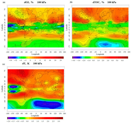
Figure A1.
Distribution of the difference in ozone concentration in % at 100 hPa (low stratosphere) (a), total ozone in % (b), and air temperature in K at 100 hPa (c) based on simulation results for scenarios with El Niño and La Niña phases.
Figure A1.
Distribution of the difference in ozone concentration in % at 100 hPa (low stratosphere) (a), total ozone in % (b), and air temperature in K at 100 hPa (c) based on simulation results for scenarios with El Niño and La Niña phases.

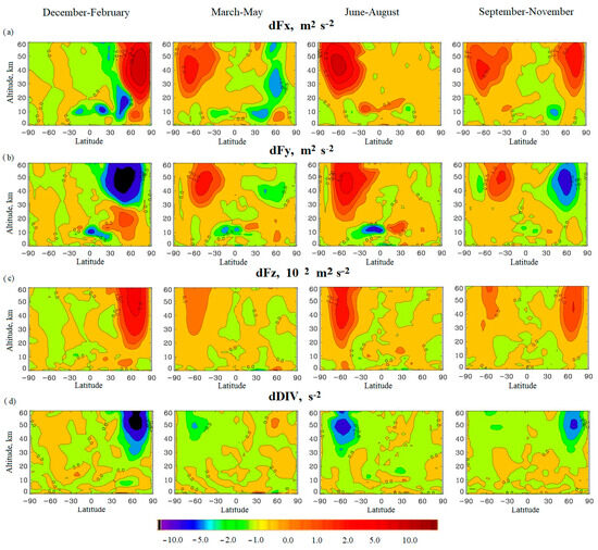
Figure A2.
Vertical zonal mean seasonal mean profiles of differences in zonal (a), meridional (b) (in m2 s−2), vertical (c) (in 102 m2 s−2), and divergence (in s−2) (d) components of the vector of Plumb wave activity based on the modeling results for the scenarios with El Niño and La Niña phases.
Figure A2.
Vertical zonal mean seasonal mean profiles of differences in zonal (a), meridional (b) (in m2 s−2), vertical (c) (in 102 m2 s−2), and divergence (in s−2) (d) components of the vector of Plumb wave activity based on the modeling results for the scenarios with El Niño and La Niña phases.
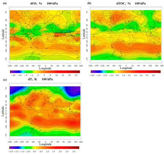
Figure A3.
Distribution of the difference in ozone concentration in % at 100 hPa (low stratosphere) altitude (a), total ozone in % (b), and air temperature in K at 100 hPa altitude (c) based on simulation results for scenarios of the end of 2010s and early 1980s.
Figure A3.
Distribution of the difference in ozone concentration in % at 100 hPa (low stratosphere) altitude (a), total ozone in % (b), and air temperature in K at 100 hPa altitude (c) based on simulation results for scenarios of the end of 2010s and early 1980s.
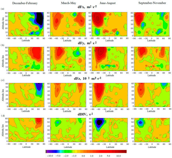
Figure A4.
Vertical zonal mean seasonal profiles of differences in zonal (a), meridional (b) (in m2 s−2), vertical (c) (in 102 m2 s−2), and divergence (in s−2) (d) components of the vector of Plumb wave activity based on modeling results for the scenarios of the late 2010s and early 1980s.
Figure A4.
Vertical zonal mean seasonal profiles of differences in zonal (a), meridional (b) (in m2 s−2), vertical (c) (in 102 m2 s−2), and divergence (in s−2) (d) components of the vector of Plumb wave activity based on modeling results for the scenarios of the late 2010s and early 1980s.

References
- Taylor, K.E.; Williamson, D.; Zwiers, F. The Sea Surface Temperature and Sea-Ice Concentracion Boundary Conditions for AMIP II Simulations, Prigram for Climate Model Diagnosis and Intercomparison; University of California: Berkeley, CA, USA, 2000; Lawrwnce Livermore National Laboratory. [Google Scholar]
- Hansen, J.; Sato, M.; Ruedy, R.; Lacis, A.; Oinas, V. Global warming in the twenty-first century: Analternative scenario. Proc. Natl. Acad. Sci. USA 2000, 97, 9875–9880. [Google Scholar] [CrossRef] [PubMed]
- Trenberth, K.; Hurrell, J.W. Decadal atmosphere-ocean variations in the Pacific. Clim. Dyn. 1994, 9, 303–319. [Google Scholar] [CrossRef]
- Collins, M.; An, S.-I.; Cai, W.; Ganachaud, A.; Guilyardi, E.; Jin, F.-F.; Jochum, M.; Lengaigne, M.; Power, S.; Timmermann, A. The impactt of global warming on the tropical Pacific Ocean and El Niño. Nat. Geosci. 2010, 3, 391–397. [Google Scholar] [CrossRef]
- Jakovlev, A.R.; Smyshlyaev, S.P.; Galin, V.Y. Interannual Variability and Trends in Sea Surface Temperature, Lower and Middle Atmosphere Temperature at Different Latitudes for 1980–2019. Atmosphere 2021, 12, 454. [Google Scholar] [CrossRef]
- Achuta Rao, K.; Sperber, K.R. Simulation of the El Nino Southern Oscillation: Results from the coupled model intercomparison project. Clim. Dyn. 2002, 19, 191–209. [Google Scholar]
- Manatsa, D.; Mukwada, G. A connection from stratospheric ozone to El Niño-Southern Oscillation. Sci. Rep. 2017, 7, 5558. [Google Scholar] [CrossRef] [PubMed]
- Guilyardi, E.; Wittenberg, A.; Fedorov, A.; Collins, M.; Wang, C.; Capotondi, A.; Oldenborgh, G.J.; van Stockdale, T. Understanding El Nino in ocean-atmosphere general circulation models. Progress and Challenges. Am. Meteorogical Soc. 2009, 90, 325–340. [Google Scholar] [CrossRef]
- Bell, C.; Gray, L.; Charlton-Perez, A.; Joshi, M.; Scaife, A. Stratospheric Communication of El Ninõ Teleconnections to European Winter. J. Clim. 2009, 22, 4083–4096. [Google Scholar] [CrossRef]
- Cagnazzo, C.; Manzini, E.; Calvo, N.; Douglass, A.; Akiyoshi, H.; Bekki, S.; Chipperfield, M.; Dameris, M.; Deushi, M.; Fischer, A.M.; et al. Northern winter stratospheric temperature and ozone responses to ENSO inferred from an ensemble of chemistry climate models. Atmos. Chem. Phys. 2009, 9, 8935–8948. [Google Scholar] [CrossRef]
- Jadin, E.A. Long-periodic cyclicity of temperature of ocean surface, temperature of low stratosphere and ozone in moderated latitudes. Meteorol. Hydrol. 1993, 5, 52–59. (In Russian) [Google Scholar]
- Newman, P.A.; Nash, E.R.; Rosenfield, J.E. What controls the temperature of the Arctic stratosphere during the spring? J. Geophys. Res. 2001, 106, 19999–20010. [Google Scholar] [CrossRef]
- Jadin, E.A. Interannual variations of ozone above Europe and anomalies of ocean temperatures in Atlantic. Meteorol. Hydrol. 1992, 7, 22–26. (In Russian) [Google Scholar]
- Jadin, E.A. Arctic oscillation and interannual variations of temperature of Atlantic and Pacific oceans. Meteorol. Hydrol. 2001, 8, 28–40. (In Russian) [Google Scholar]
- Hu, D.; Tian, W.; Xie, F.; Shu, J.; Dhomse, S. Effects of meridional sea surface temperature changes on stratospheric temperature and circulation. Adv. Atmos. Sci. 2014, 31, 888–900. [Google Scholar] [CrossRef]
- Smyshlyaev, S.P.; Pogoreltsev, A.I.; Galin, V.J. Influence of wave activity on gaseous composition of stratosphere of polar regions. Geomagn. Aeron. 2016, 56, 102–116. [Google Scholar] [CrossRef]
- Horel, J.D.; Wallace, J.M. Planetary scale atmospheric phenomena associated with the Southern Oscillation. Mon. Weather. Rev. 1981, 109, 813–829. [Google Scholar] [CrossRef]
- Iza, M.; Calvo, N.; Manzini, E. The stratospheric pathway of La Nina. J. Clim. 2016, 29, 8899–8914. [Google Scholar] [CrossRef]
- Domeisen, D.I.; Garfinkel, C.; Butler, A.H. The teleconnection of El Nino southern oscillation to the stratosphere. Rev. Geophys. 2019, 57, 5–47. [Google Scholar] [CrossRef]
- Polvani, L.M.; Sun, L.; Butler, A.H.; Richter, J.H.; Deser, C. Distinguishing stratospheric sudden warmings from ENSO as key drivers of wintertime climate variability over the North Atlantic and Eurasia. J. Clim. 2017, 30, 1959–1969. [Google Scholar] [CrossRef]
- Garfinkel, C.I.; Butler, A.H.; Waugh, D.W.; Hurwitz, M.M. Why might SSWs occur with similar frequency in El Nino and La Nina winters? J. Geophys. Res. 2012, 117, 106. [Google Scholar] [CrossRef]
- García-Herrera, R.; Calvo, N.; Garcia, R.R.; Giorgetta, M.a. Propagation of ENSO temperature signals into the middle atmosphere: A comparison of two general circulation models and ERA-40 reanalysis data. J. Geophys. Res. 2006, 111, D06101. [Google Scholar] [CrossRef]
- Garfinkel, C.I.; Hartmann, D.L. Effects of the El Niño–Southern Oscillation and the Quasi-Biennial Oscillation on polar temperatures in the stratosphere. J. Geophys. Res. 2007, 112, D19112. [Google Scholar] [CrossRef]
- Butler, A.H.; Polvani, L.M. El Niño, La Niña, and stratospheric sudden warmings: A reevaluation in light of the observational record. Geophys. Res. Lett. 2011, 38, 13. [Google Scholar] [CrossRef]
- Ineson, S.; Scaife, A.A. The role of the stratosphere in the European climate response to El Niño. Nat. Geosci. 2009, 2, 32–36. [Google Scholar] [CrossRef]
- Butler, A.H.; Polvani, L.M.; Deser, C. Separating the stratospheric and tropospheric pathways of El Niño—Southern Oscillation teleconnections. Environ. Res. Lett. 2014, 9, 024014. [Google Scholar] [CrossRef]
- Butler, A.H. El Niño and the stratospheric polar vortex//NOAA Climate.gov (Science & Information for a Climate—Smart Nation). Available online: https://www.climate.gov (accessed on 28 April 2016).
- Sassi, F.; Kinnison, D.; Boville, B.A.; Garcia, R.R.; Roble, R. Effect of El Niño—Southern Oscillation on the dynamical, thermal, and chemical structure of the middle atmosphere. J. Geophys. Res. Atmos. 2004, 109, D17108. [Google Scholar] [CrossRef]
- Hu, J.; Shen, Y.; Deng, J.; Jia, Y.; Wang, Z.; Li, A. Revisiting the Influence of ENSO on the Arctic Stratosphere in CMIP5 and CMIP6 Models. Atmosphere 2023, 14, 785. [Google Scholar] [CrossRef]
- Vargin, P.N.; Kolennikova, M.A.; Kostrykin, S.V.; Volodin, E.M. Impact of sea surface temperature anomalies in the equatorial and North Pacific on the arctic stratosphere according to the INM CM5 climate model simulations. Russ. Meteorol. Hydrol. 2021, 46, 1–9. [Google Scholar] [CrossRef]
- Zubov, V.A.; Rozanova, I.V.; Kiselev, A.A.; Karol, I.L.; Rozanov, E.V.; Egorova, T.A.; Schmutz, V. Simulation of Changes in Global Ozone and Atmospheric Dynamics in the 21st Century with the Chemistry-Climate Model SOCOL. Izv. Atmos. Ocean. Phys. 2011, 47, 301–312. [Google Scholar] [CrossRef]
- Volodin, E.M.; Gritsun, A.S. Simulation of Possible Future Climate Changes in 21 Century with Climate Model INM-CM5. Izv. Atmos. Ocean. Phys. 2020, 56, 218–228. [Google Scholar] [CrossRef]
- Plumb, R.A. On the Three-Dimensional Propagation of Stationary Waves. J. Atmos. Sci. 1985, 42, 217–229. [Google Scholar] [CrossRef]
- Kinoshita, T.; Tomikawa, Y.; Sato, K. On the Three-Dimensional Residual Mean Circulation and Wave Activity Flux of the Primitive Equations. J. Meteorol. Soc. Jpn. 2010, 88, 373–394. [Google Scholar] [CrossRef]
- Galin, V.Y.; Smyshlyaev, S.P.; Volodin, E.M. Combined Chemistry–Climate Model of the Atmosphere. Izv. Atmos. Ocean. Phys. 2007, 43, 399–412. [Google Scholar] [CrossRef]
- Smyshlyaev, S.P.; Galin, V.Y.; Shaariibuu, G.; Motsakov, M.A. Modeling the Variability of Gas and Aerosol Components in the Stratosphere of Polar Regions. Izv. Atmos. Ocean. Phys. 2010, 46, 265–280. [Google Scholar] [CrossRef]
- Smyshlyaev, S.P.; Galin, V.Y.; Blakitnaya, P.A.; Jakovlev, A.R. Numerical Modeling of the Natural and Manmade Factors Influencing Past and Current Changes in Polar, Mid-Latitude and Tropical Ozone. Atmosphere 2020, 11, 76. [Google Scholar] [CrossRef]
- Smyshlyaev, S.P.; Geller, M.A.; Yudin, V.A. Sensitivity of model assessments of high-speed civil transport effects on stratospheric ozone resulting from uncertainties in the NOx production from lightning. J. Geophys. Res. 1999, 104, 26401–26417. [Google Scholar] [CrossRef]
- Sukhodolov, T.; Rozanov, E.; Ball, W.T.; Schmutz, W.; Peter, T.; Bais, A.; Tourpali, K.; Shapiro, A.I.; Telford, P.; Smyshlyaev, S.; et al. Evaluation of simulated photolysis rates and their response to solar irradiance variability. J. Geophys. Res. 2016, 121, 6066–6084. [Google Scholar] [CrossRef]
- Dianskii, N.A.; Galin VYa Gusev, A.V.; Volodin, E.M.; Iakovlev, N.G.; Smyshlyaev, S.P. The model of the Earth system developed at the INM RAS. Russ. J. Numer. Anal. Math. Model. 2010, 25, 419–429. [Google Scholar] [CrossRef]
- Weather and Climate Change. [Electronic Resource]/Met Office. Available online: http://https://www.metoffice.gov.uk/hadobs/hadgem_sst/data/download.html (accessed on 20 March 2022).
- Jakovlev, A.R.; Smyshlyaev, S.P. The Impact of the Tropical Sea Surface Temperature Variability on the Dynamical Processes and Ozone Layer in the Arctic Atmosphere. Meteorology 2024, 3, 36–69. [Google Scholar] [CrossRef]
- Jakovlev, A.R.; Smyshlyaev, S.P. Numerical Simulation of World Ocean Effects on Temperature and Ozone in the Lower and Middle Atmosphere. Russ. Meteorol. Hydrol. 2019, 44, 594–602. [Google Scholar] [CrossRef]
- Jakovlev, A.R.; Smyshlyaev, S.P. Impact of the Southern Oscillation on Arctic Stratospheric Dynamics and Ozone Layer. Izv. Atmos. Ocean. Phys. 2019, 55, 86–99. [Google Scholar] [CrossRef]
- Gelaro, R.; McCarty, W.; Suarez, M.J.; Todling, R.; Molod, A.; Takacs, L.; Randles, C.; Darmenov, A.; Bosilovich, M.; Reichle, R.; et al. The Modern-Era Retrospective Analysis for Research and Applications, Version 2 (MERRA-2). J. Clim. 2017, 30, 5419–5454. [Google Scholar] [CrossRef] [PubMed]
- Garfinkel, C.I.; Hartmann, D.L. Different ENSO teleconnections and their effects on the stratospheric polar vortex. J. Geophys. Res Atmos. 2008, 113, D18114. [Google Scholar] [CrossRef]
- Kolennikova, M.; Gushchina, D. Revisiting the Contrasting Response of Polar Stratosphere to the Eastern and Central Pacific El Niños. Atmosphere 2022, 13, 682. [Google Scholar] [CrossRef]
- Gushchina, D.; Kolennikova, M.; Dewitte, B.; Yeh, S.-W. On the relationship between ENSO diversity and the ENSO atmospheric teleconnection to high-latitudes. Int. J. Climatol. 2021, 42, 1303–1325. [Google Scholar] [CrossRef]
- Prentice, I.C.; Farquhar, G.D.; Fasham, M.J.R.; Goulden, M.L.; Heimann, M.; Jaramillo, V.J.; Kheshgi, H.S.; Le Quéré, C.; Scholes, R.J.; Wallace, D.W.R. The carbon cycle and atmospheric carbon dioxide. In Third Assessment Report of the Intergovernmental Panel on Climate Change. Climate Change 2001: The Scientific Basis; IPCC, Ed.; Cambridge University Press: Cambridge, UK, 2001; pp. 183–238. [Google Scholar]
- Stevenson, S.; Fox-Kemper, B. Understanding the ENSO–CO2 Link Using Stabilized Climate Simulations. J. Clim. 2012, 25, 7917–7936. [Google Scholar] [CrossRef]
- Polvani, L.M.; Waugh, D.W. Upward wave activity flux as a precursor to extreme stratospheric events and subsequent anomalous surface weather regimes. J. Clim. 2004, 17, 3548–3554. [Google Scholar] [CrossRef]

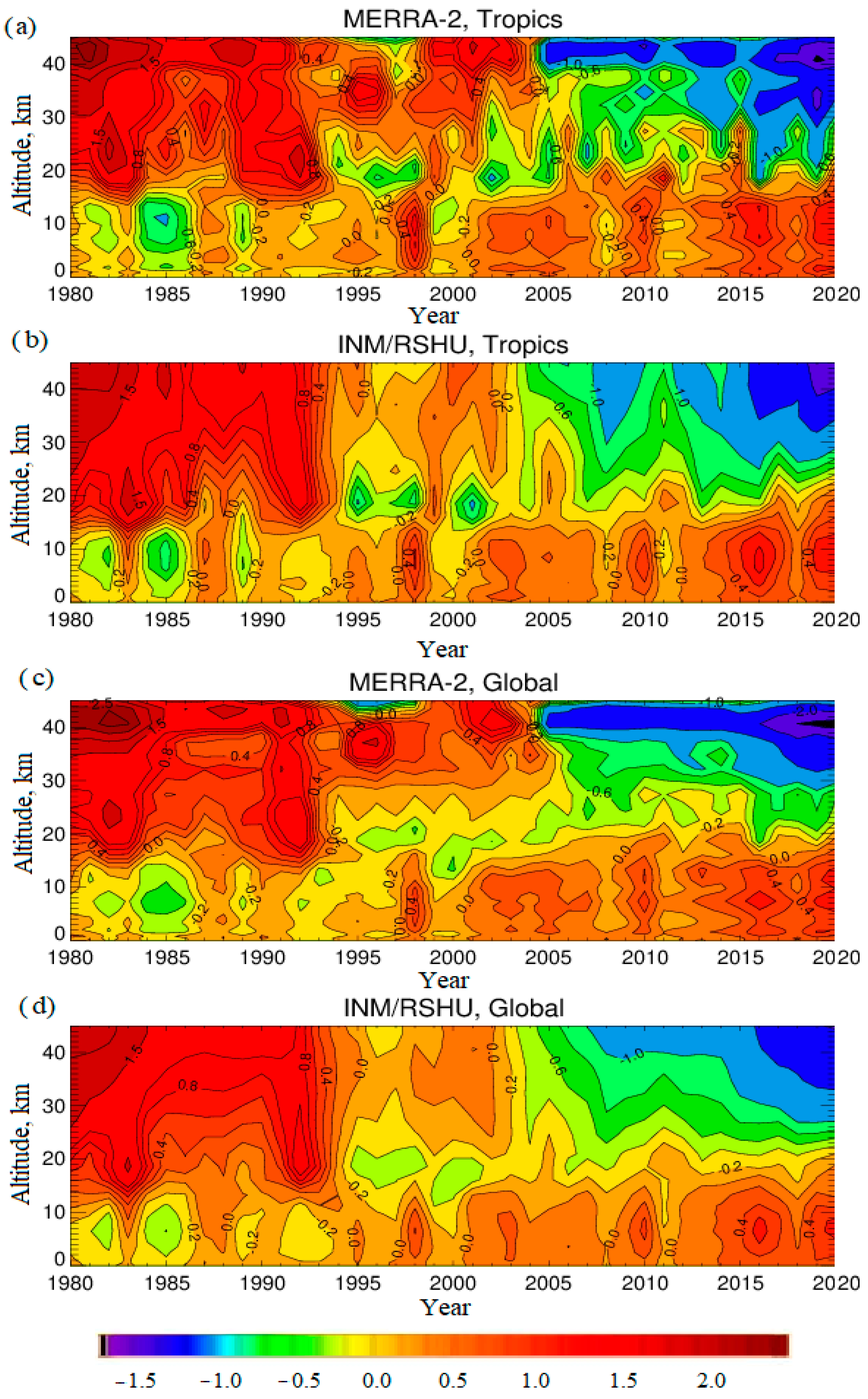
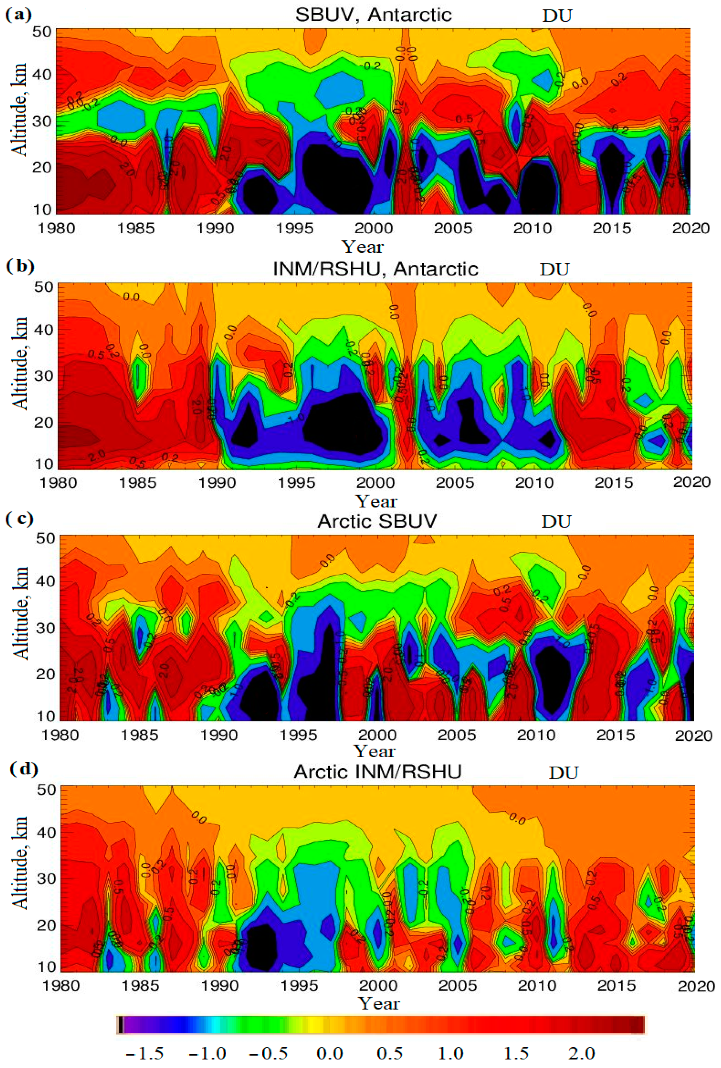
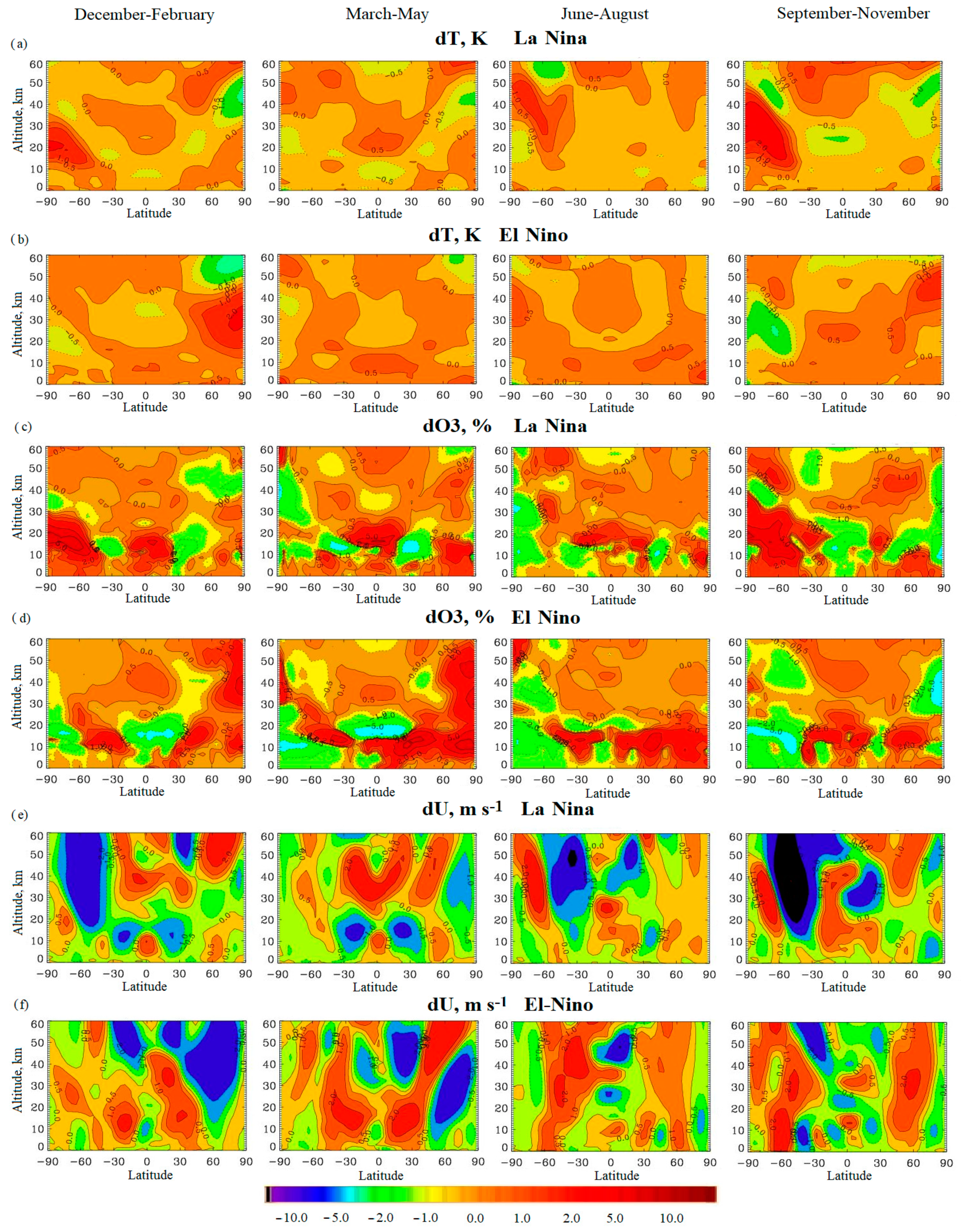
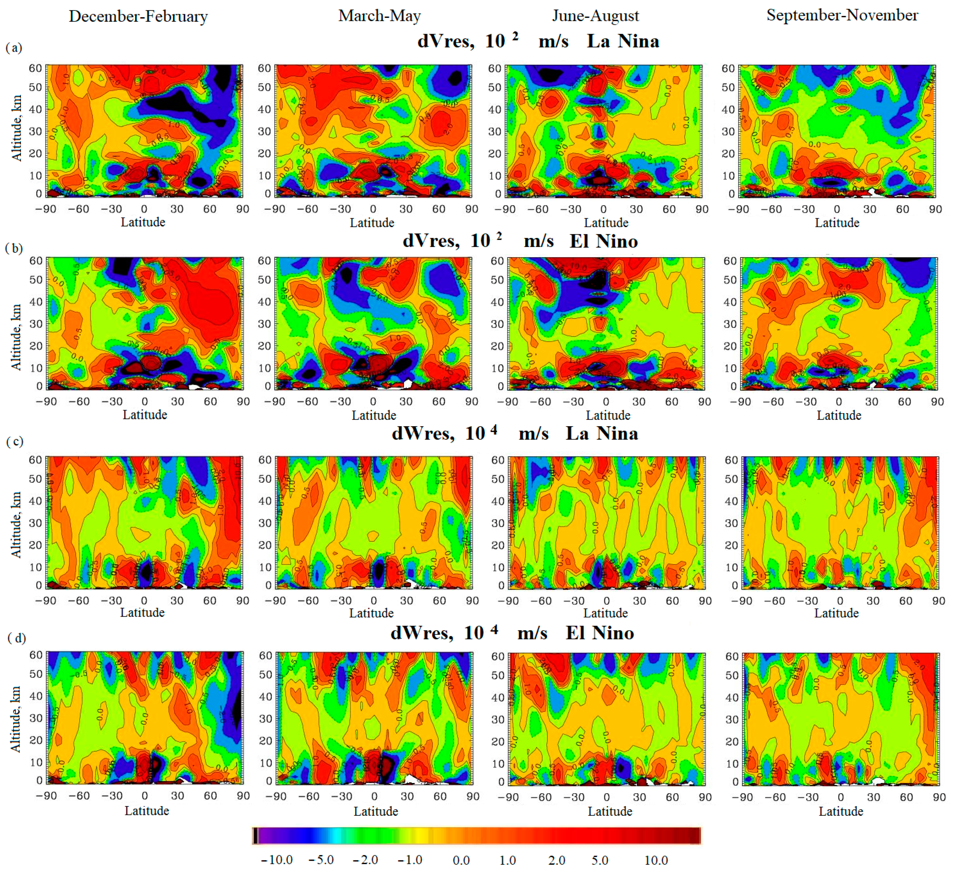
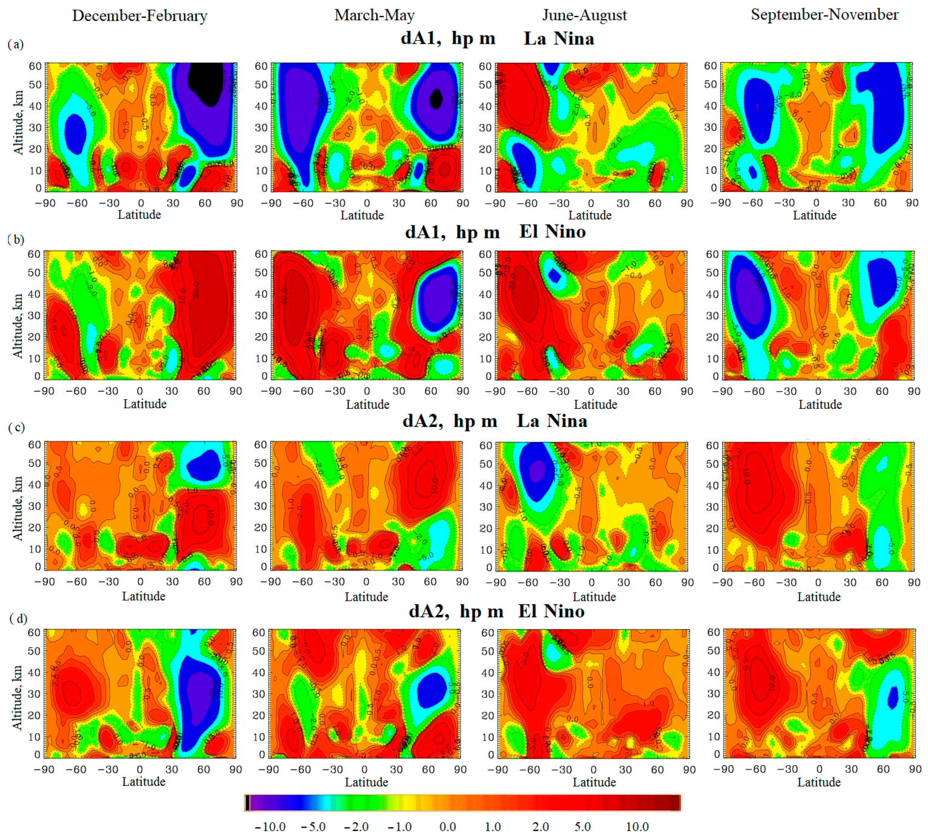

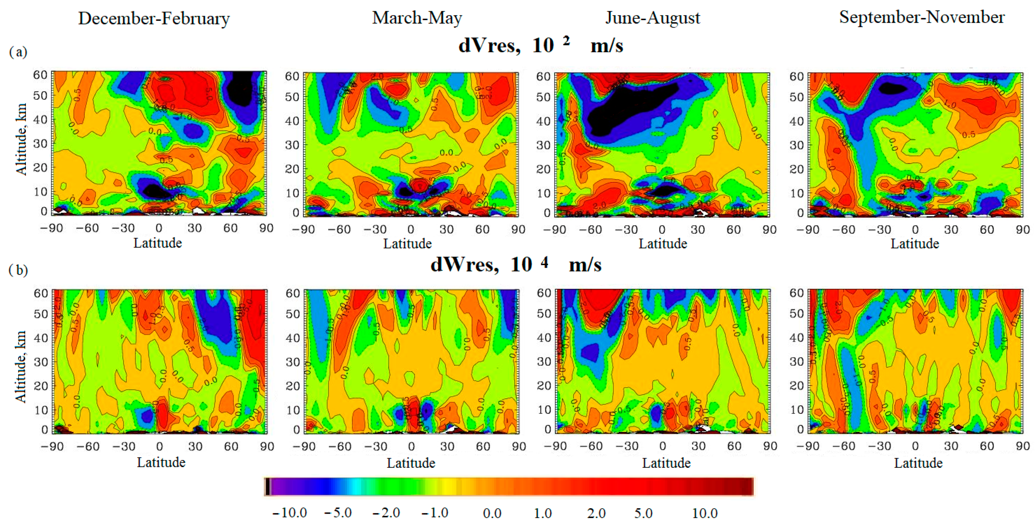
Disclaimer/Publisher’s Note: The statements, opinions and data contained in all publications are solely those of the individual author(s) and contributor(s) and not of MDPI and/or the editor(s). MDPI and/or the editor(s) disclaim responsibility for any injury to people or property resulting from any ideas, methods, instructions or products referred to in the content. |
© 2024 by the authors. Licensee MDPI, Basel, Switzerland. This article is an open access article distributed under the terms and conditions of the Creative Commons Attribution (CC BY) license (https://creativecommons.org/licenses/by/4.0/).