Article

Multi-Row Turbomachinery Aerodynamic Design Optimization by an Efficient and Accurate Discrete Adjoint Solver

School of Power and Energy, Northwestern Polytechnical University, Xi’an 710072, China
*
Author to whom correspondence should be addressed.
Aerospace 2023, 10(2), 106; https://doi.org/10.3390/aerospace10020106
Submission received: 30 December 2022 / Revised: 18 January 2023 / Accepted: 18 January 2023 / Published: 21 January 2023
(This article belongs to the Special Issue Adjoint Method for Aerodynamic Design and Other Applications in CFD)

Abstract

:
This paper proposes an approach that combines manual differentiation (MD) and automatic differentiation (AD) to develop an efficient and accurate multi-row discrete adjoint solver. In this approach, the structures of adjoint codes generated using an AD tool are first analyzed. Then, the AD-generated codes are manually adjusted to reduce memory and CPU time consumption. This manual adjustment is performed by replacing the automatically generated low-efficient differentiated codes with manually developed ones. To demonstrate the effectiveness of the proposed approach, the single-stage transonic compressor–NASA Stage 35 and the 1.5-stage Aachen turbine–are used. The solution information exchange at a rotor-stator/stator-rotor interface is achieved by a conservative, non-reflective, and robust discrete adjoint mixing plane method. The results show that the discrete adjoint solver developed by hybrid automatic and manual differentiation is more economical in computational cost than that developed purely by an AD tool and has higher sensitivity accuracy than the adjoint solver with the constant eddy viscosity (CEV) assumption. Moreover, the multi-row turbomachinery design optimizations can be efficiently performed by the discrete adjoint solver developed by the hybrid automatic and manual differentiation.

1. Introduction

Modern advanced turbomachines are quite often designed to have complex three-dimensional features such as lean, twist, and sweep. Therefore, hundreds or even thousands of design variables are required to parameterize blade profiles. The gradient-free method [1] and the gradient-based method with sensitivity calculated using a direct method (the finite difference method et al.), which is too computationally intensive even with the currently available computing resources. The adjoint method is an efficient gradient calculation method and suits gradient-based design optimizations with a large number of design variables and a limited number of objective functions and constraints. At each design cycle, design sensitivity calculation requires the flow and adjoint fields to be computed once only regardless of the number of design variables. In the past three decades, the adjoint method applied to both radial [2] and axial [3] turbomachinery design optimizations has been extended from single-row [4] to multi-row environments [5,6], from steady [7] to unsteady [8,9,10] simulations, and from single [11] to multiple disciplines [12].
With the development of the adjoint method, two types appear: continuous [13,14] and discrete [15]. The difference between the two types lies in the sequence in which the linearization, adjoint, and discretization processes are performed. The discrete adjoint method first discretizes the flow governing equations and then linearizes the corresponding flow solver’s subroutines, followed by an adjoint operation. The continuous adjoint method starts with the linearization of the partial differential flow governing equation. The adjoint equation in differential form is then derived and discretized to obtain the solvable discrete equation. Because of the higher sensitivity accuracy compared with the continuous adjoint method, the discrete adjoint method will be studied in this work.
The development of discrete adjoint solvers can be achieved by manual differentiation (MD) [16] or with the aid of automatic differentiation (AD) [17,18]. At the early stage of the adjoint method development, manual differentiation was mainly adopted to develop a discrete adjoint solver due to the immaturity of AD techniques. The main advantage of such a discrete adjoint solver developed by manual differentiation is the high computational efficiency. Its computational cost is comparable to that required by the corresponding flow solver. However, there are some drawbacks to the manual differentiation approach. First, the linearization of a discrete flow equation and the derivation of the corresponding adjoint equation is tedious and error-prone. Second, it is difficult to manually linearize the turbulence model equations and derive the adjoint counterparts. Therefore, the constant eddy viscosity assumption (CEV) [19] that freezes the eddy viscosity is adopted. This is found to adversely affect adjoint solution stability, adjoint solution convergence, and adjoint sensitivity accuracy. Third, the maintainability and synchronization between the flow and adjoint solvers are poor. When any change is made to the flow solver, there is a need to update the corresponding adjoint solver. Otherwise, inconsistency between the two solvers can lead to solution inaccuracy and even solution instability of the adjoint part. Synchronizing the two solvers manually requires complete knowledge of the two solvers, which is often difficult in an industrial environment.
Apart from the manual differentiation, the AD tool is another way to develop a discrete adjoint solver. At present, there are two types of AD tool-operator overloading [20] and source code transformation [21]. The former does not produce adjoint codes explicitly. It computes the derivative information using the overloaded library after the original data type is replaced with a new one that contains the derivative information. The overloaded library defines the overloaded type and arithmetic operations. The latter takes subroutines of a flow solver as the input together with auxiliary information about the input and output variables of those subroutines, and then adjoint subroutines are produced automatically and almost instantly. Compared with operator overloading, source code transformation is less development-intensive. Programmers can trace back the adjoint codes to know detailed information about the differentiated process. Due to the above merit, the source code transformation AD tool-TAPENADE will be used in our work.
When TAPENADE is adopted to develop a discrete adjoint solver, first there is a need to be clear about the input and output of subroutines to be differentiated. Then, the reverse mode is selected to differentiate the subroutines of a flow solver. Finally, the corresponding adjoint codes are generated automatically. The whole process is easy to understand and work on, but the approach has some drawbacks. First, the computational efficiency of the adjoint codes generated using an AD tool tends to be quite low. According to reference [21], the ratio of the adjoint solver runtime to that of the flow solver is 5–10. Second, the adjoint codes can be complicated and unable to be run in parallel due to race conditions. For cases with millions or even billions of grid nodes, too much wall clock time [22,23] will be required for optimization using such an adjoint solver.
To overcome the drawbacks of a discrete adjoint solver developed purely by an AD tool, considerable effort has been made in the past twenty years. Giles et al. [24] proposed the selective use of AD in developing a discrete adjoint solver. In his approach, the flow solver’s subroutines are selectively differentiated in a reverse mode by using the AD tool, and then resultant adjoint codes are manually assembled. Compared with the differentiation of the subroutines of a complete flow solver, a discrete adjoint solver developed in this approach is more efficient in terms of its computational cost. Mader et al. [25] followed the same principle and proposed the ADjoint approach for the rapid development of discrete adjoint solvers. However, Muller et al. [22] pointed out that the computational efficiency of this kind of adjoint solver heavily depends on the flow solver’s data structures. In some situations, the computational cost required by the discrete adjoint solver is over three times that required by the flow solver. To improve the computational efficiency of discrete adjoint solvers developed by using AD tools, he proposed a series of strategies to modify the flow solver’s structures, such as avoiding using the same symbol to represent different variables and putting a do-loop out of subroutines. The modified flow solver’s subroutines will be differentiated and manually assembled again to obtain the modified adjoint solver. Although these strategies are effective, too many modifications to the flow solver’s codes are required. Sometimes, the computational efficiency of modified adjoint codes is still low even though the modifications to the flow solver’s codes are made. Therefore, it is urgent to propose new approaches to develop efficient discrete adjoint solvers with the aid of AD.
By analyzing the raw adjoint codes generated by the AD tool-TAPENADE, it can be found that there are plenty of PUSH and POP functions. They are used to record and retrieve the intermediate variables. These extra function calls will affect the computational efficiency of the adjoint codes. Moreover, these functions make the adjoint codes difficult to read and unable to be run in parallel. The latter is caused by race conditions among different threads/processors.
In this work, an approach that combines manual and automatic differentiation is proposed for developing efficient discrete adjoint solvers. This approach keeps the structures of an original flow solver’s codes unchanged and directly adjusts the structures of AD-generated raw adjoint codes. Three main steps are required by such an approach. First, use the AD tool to differentiate the flow solver’s subroutines and obtain the corresponding adjoint codes. Second, analyze the raw adjoint codes and figure out the functionality of each part. If PUSH/POP function pairs are not called in the raw adjoint codes, there is no need to do the following modifications. Otherwise, replace the adjoint codes related to PUSH/POP functions with manually developed codes. The following part will introduce how to develop the manually differentiated codes. The modified adjoint codes are expected to be easier to read and more efficient in computational cost. Moreover, the discrete adjoint solver developed by hybrid manual and automatic differentiation can still handle the turbulence model equations, ensuring accurate sensitivity calculation. To demonstrate the effectiveness of the hybrid discrete adjoint method, the single-stage transonic compressor-NASA Stage 35 [26] and the 1.5-stage Aachen turbine [27] are used. For the two multi-row cases, the information exchange at a rotor-stator/stator-rotor interface is achieved by a conservative, non-reflective and robust mixing plane method for the flow solver [28] and a corresponding discrete adjoint mixing plane method for the adjoint solver.

2. Numerical Schemes and Boundary Conditions

The steady Reynolds-averaged Navier-Stokes (RANS) equation in a cylindrical coordinate system can be written as follows
( F V x ) x + ( G U v g , θ V θ ) r θ + r ( H V r ) r r = S
where U is the flow variable vector; x, θ , and r are the axial, circumferential, and radial coordinates, respectively; F, G, and H are the convective flux vectors; V x , V θ , and V r are the viscous flux vectors; S is the source term vector; and v g , θ is the grid velocity in the circumferential direction.

2.1. Numerical Schemes

Equation (1) is solved using the in-house finite volume solver—TurboXD [29]. The one-equation Spalart-Allmaras turbulence model [30] is used in the solver to compute the eddy viscosity. The pseudo-time integration is achieved by a hybrid implicit lower upper symmetric Gauss-Seidel (LU-SGS) and explicit four-stage Runge-Kutta method [29]. The LU-SGS method is used as an implicit residual smoother to increase the Courant number, leading to faster convergence. To further accelerate convergence, the local time-stepping method is applied. The convective fluxes are calculated using the central scheme with the blending of first-order and third-order artificial dissipation terms, also known as the Jameson-Turkel-Schmidt (JST) scheme [31]. The spatial derivatives of the flow variable to the grid coordinates are computed by the Gauss-Green formula, and then these terms are used to compute viscous fluxes.

2.2. Boundary Conditions

There are five types of boundary conditions for multi-row cases: inlet, outlet, solid wall, geometric periodic boundaries, and rotor-stator/stator-rotor interfaces. At both the inlet and outlet, the subsonic boundary conditions are applied in our work. At the inlet, the radial profiles of total pressure, total temperature, and two flow angles are specified. At the outlet, the back pressure at the hub or casing is specified, and then the simple radial equilibrium is used to determine the static pressure at the other radial locations. To reduce the mesh density around a solid wall and thus save computational cost, the slip wall boundary condition and the wall function are applied to solid wall boundaries. At the geometric periodic boundaries, the periodic boundary condition is applied. At a rotor-stator/stator-rotor interface, a flux-conservative robust mixing plane method is used [28].

3. Adjoint Principle

If the goal of turbomachinery aerodynamic design optimization is to reduce aerodynamic loss, the corresponding objective function can be isentropic efficiency or entropy generation rate, which can be expressed in the following symbolic form
I = I ( U , α )
where I is the objective function; U and α are the flow and design variable vectors, and they are connected by Euler/Navier–Stokes equations
R ( U , α ) = 0
where R is the residual.
For gradient-based design optimizations, there is a need to compute the sensitivity of I to α . According to the chain rule, we have
d I d α = I α + I U d U d α
In Equation (4), the calculations of I α and I U do not involve the solution of equations and can be accomplished analytically or numerically. However, the calculation of d U d α requires the solution of flow governing equations in one way or another and accounts for the most computational cost. If a direct method such as the finite difference method (FDM) is used to calculate this term, the number of computational fluid dynamics (CFD) computations required is proportional to the number of design variables. For cases with hundreds or even thousands of design variables, the required computational cost is prohibitive.
The key of the adjoint method is to avoid direct calculation of d U d α in sensitivity evaluation. Linearizing Equation (3) and making some arrangements leads to
d U d α = ( R U ) 1 R α
Substitute Equation (5) into Equation (4), and we have
d I d α = I α + λ T R α
where λ is the adjoint variable vector and satisfies the following adjoint equation
( R U ) T λ = ( I U ) T
Since the adjoint equation is free from d U d α , the number of equations to be solved by the adjoint method is independent of the number of design variables. To obtain the sensitivities of one objective function or constraint to all design variables, the flow field and the adjoint field need to be computed once only. For cases where the number of objective functions or constraints is far fewer than the number of design variables, the adjoint method will be more efficient in computing sensitivities than the direct method.

4. Automatic Differentiation

If the adjoint method is used to compute sensitivities, there is a need to develop the corresponding adjoint solver. With the development of automatic differentiation techniques, more and more attention has been paid to the development of discrete adjoint solvers using AD tools.

4.1. Forward and Backward Modes

Automatic differentiation has two modes: forward mode and backward mode. The former is used to produce a linearized code, and the latter is used to produce an adjoint code. Assume that there is a chain relationship such as:
α U ( α ) I ( U ( α ) )
To obtain the sensitivity of I to α , the forward mode starts from the perturbation of α , and then the differentiated results of U and I are computed successively. The chain relationship of the forward mode can be expressed as:
α t U t = d U d α α t I t = d I d U U t = d I d U d U d α α t = d I d α α t
If α t is set to 1, I t will represent the sensitivity of I with respect to α .
Different from the forward mode, the backward mode starts from the perturbation of I, and then the differentiated results of U and α are computed step by step. The chain relationship is given as follows:
I a U a = ( d I d U ) T I a α a = ( d U d α ) T U a = ( d I d U d U d α ) T I a = ( d I d α ) T I a
If I a is set to 1, α a will represent the transpose of sensitivity.
From the above introduction, it can be found that the differentiated results from both modes are identical. When the flow solver’s subroutines are fully differentiated, the discrete adjoint solver should have the same sensitivity convergence history and asymptotic convergence rate of residual as the linearized solver. However, the processes of differentiation are different for the two modes, leading to the following differences.
First, the reverse mode can obtain the sensitivity of one objective function or constraint to all design variables at the same time. However, the sensitivities of more than one objective function and/or constraint to one design variable can be computed in one go in the forward mode. When the number of design variables is far bigger than that of objective functions/constraints, the reverse mode is more efficient in computing sensitivity than the forward mode, and vice versa.
Second, the computational sequence of the backward mode is reversed and thus complex compared with that of the forward mode. This leads to tedious adjoint codes. With the increasing complexity of functions, the computational efficiency of the adjoint codes will dramatically reduce. In the following part, the causes of the deteriorated computational efficiency of the adjoint codes will be analyzed in detail.

4.2. Problem Description and Analysis

As an AD tool generates adjoint codes in reverse mode, there is a need to record intermediate variables for later use. In the adjoint codes, this is achieved by stack operation. First, the intermediate variables are calculated and pushed into the stack using the PUSH operation in its original forward sweep. Second, the intermediate variables are retrieved from the stack using the POP operation in a backward sweep. According to data types of intermediate variables, there are three pairs of PUSH/POP functions. PUSHCONTROL/POPCONTROL functions are for conditional branches. PUSHREAL4/POPREAL4 are for single-precision floating-point numbers. PUSHINTEGER/POPINTEGER are for integrals. Since the functionalities of PUSHREAL4/POPREAL4 and PUSHINTEGER/POPINTEGER are similar to each other, only two simple cases will be given to introduce PUSH and POP operations.

4.2.1. Conditional Branches

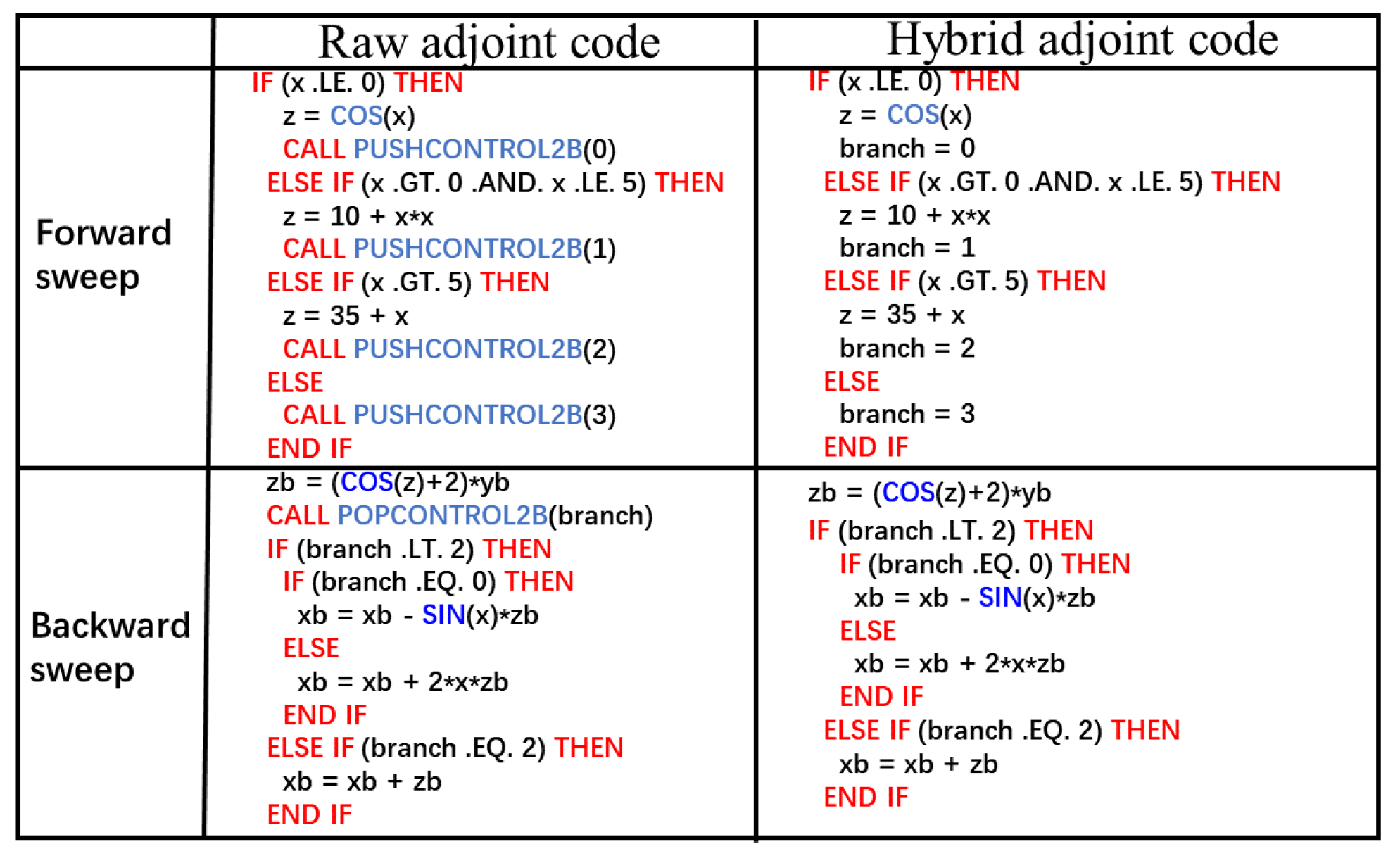
The PUSHCONTROL/POPCONTROL mainly exists in the conditional statements, as shown in Figure 1. In the primal code, x is the independent variable, z is an intermediate variable, and y is the dependent variable. It can be seen in the primal code that the i f statement is used to evaluate z and different z s will affect the dependent variable y. In the raw adjoint code, integers (0, 1, 2, and 3 in this case) are used to represent the branches of the i f statement. The PUSHCONTROL2B function is called to record the branches in a forward sweep. In a backward sweep, the recorded branch statuses are retrieved by calling the POPCONTROL2B function. It can be seen from this example that PUSHCONTROL2B/POPCONTROL2B functions are used to record and retrieve conditional branches in the raw adjoint code.

4.2.2. Reals/Integrals

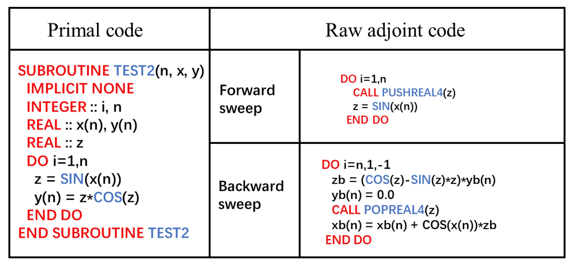
Figure 2 shows the raw adjoint code for recording and retrieving single-precision floating-point numbers. The primal code only has one do loop. In the do loop, the intermediate variable z is computed first and then used to compute the dependent variable y. In the raw adjoint code, two do loops are produced. The first is to calculate z and push it into a stack just before overwriting. Later, these values are retrieved by a pop operation in the second do loop and used to compute sensitivity. It can be seen in the raw adjoint code that the number of PUSH/POP function calls increases proportionally with the loop count n. For a large n, the extra PUSH/POP function calls will greatly increase the computational cost.

5. Hybrid Automatic and Manual Differentiation

In the raw adjoint codes, the number of PUSH/POP function calls is mainly related to the number of intermediate variables and conditional branches. The extra function calls can deteriorate the computational efficiency of adjoint codes. Referring to the two cases explained above, strategies for the development of more efficient hybrid adjoint codes will be introduced in the following part.

5.1. Strategy One: Directly Evaluate Conditional Branches

This strategy is proposed to eliminate the inefficient PUSH/POP operations as explained in case 1 and Figure 1. In the raw adjoint code, the branch status is pushed into a stack. The proposed strategy directly evaluates and saves a branch status in a variable rather than uses a stack operation involving PUSH/POP functions. Figure 3 presents the hybrid adjoint code for case 1. It can be seen that the hybrid adjoint code is free from PUSH/POP function calls and thus more efficient in computational cost.

5.2. Strategy Two: Directly Evaluate Intermediate Variables

The second strategy is about how to eliminate inefficient PUSH/POP operations for intermediate variables as explained in case 2 and Figure 2. Instead of pushing the values of intermediate variables into a stack in a forward sweep, it is proposed to calculate the intermediate variables on the fly in the backward sweep. This strategy makes the original forward sweep calculation redundant, and thus the forward sweep has to be removed completely. One needs to bear in mind when applying this strategy: first, the involved intermediate variables do not have a dependence on each other; second, the intermediate variables should be put in the correct location in the backward sweep. In the hybrid adjoint code (see Figure 4), the calculation of the intermediate variable z is put at the top of the backward sweep. Compared with the raw adjoint code, the hybrid adjoint code is free from PUSHREAL4/POPREAL4 function calls. The computational cost required by the hybrid adjoint code will be reduced by a great deal.

5.3. Strategy for Real-Life Adjoint Codes

The above two simple cases are used to introduce the two strategies for the hybrid automatic and manual differentiation approach. For real-life codes, such as those of a CFD solver, different types of intermediate variables exist in one subroutine at the same time, leading to the calls of different PUSH/POP function pairs simultaneously in this subroutine. Therefore, a combination of the two strategies is required to develop efficient hybrid adjoint codes.
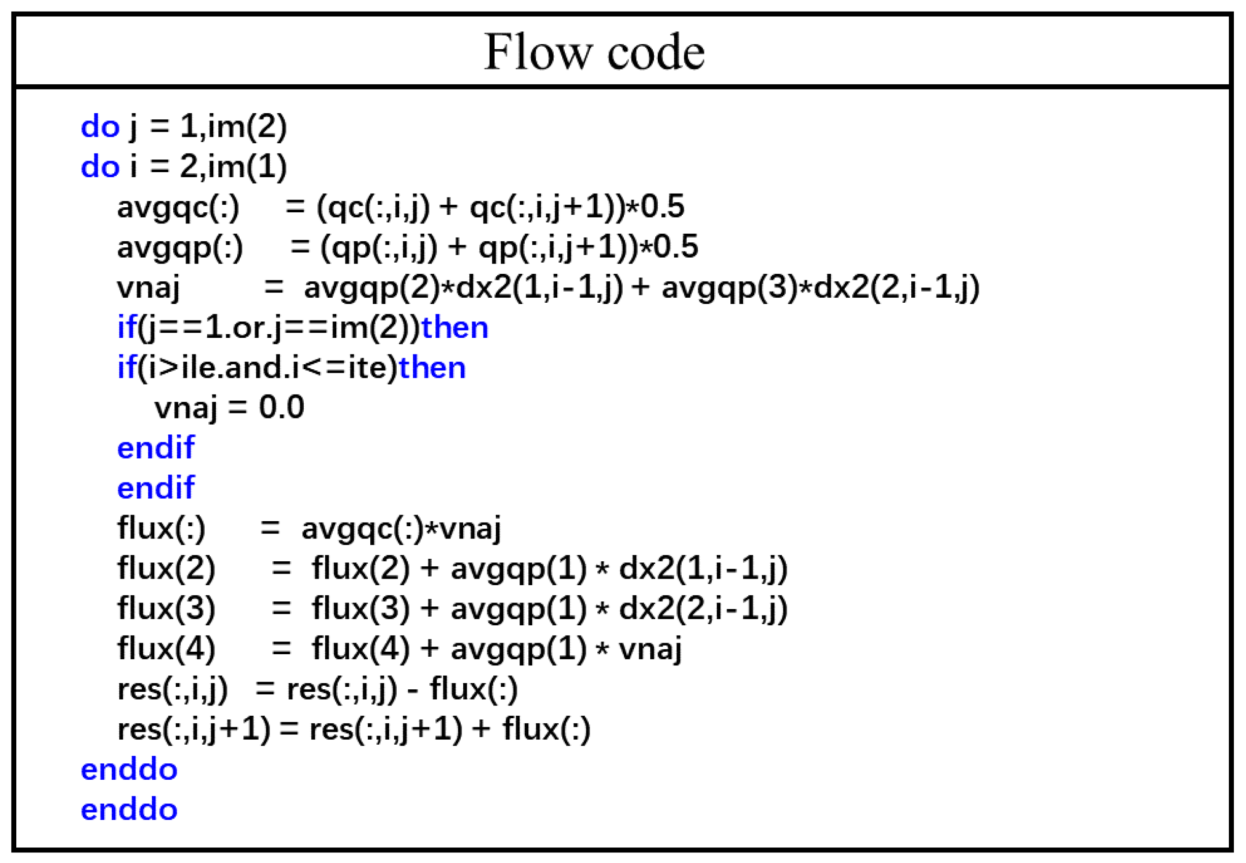
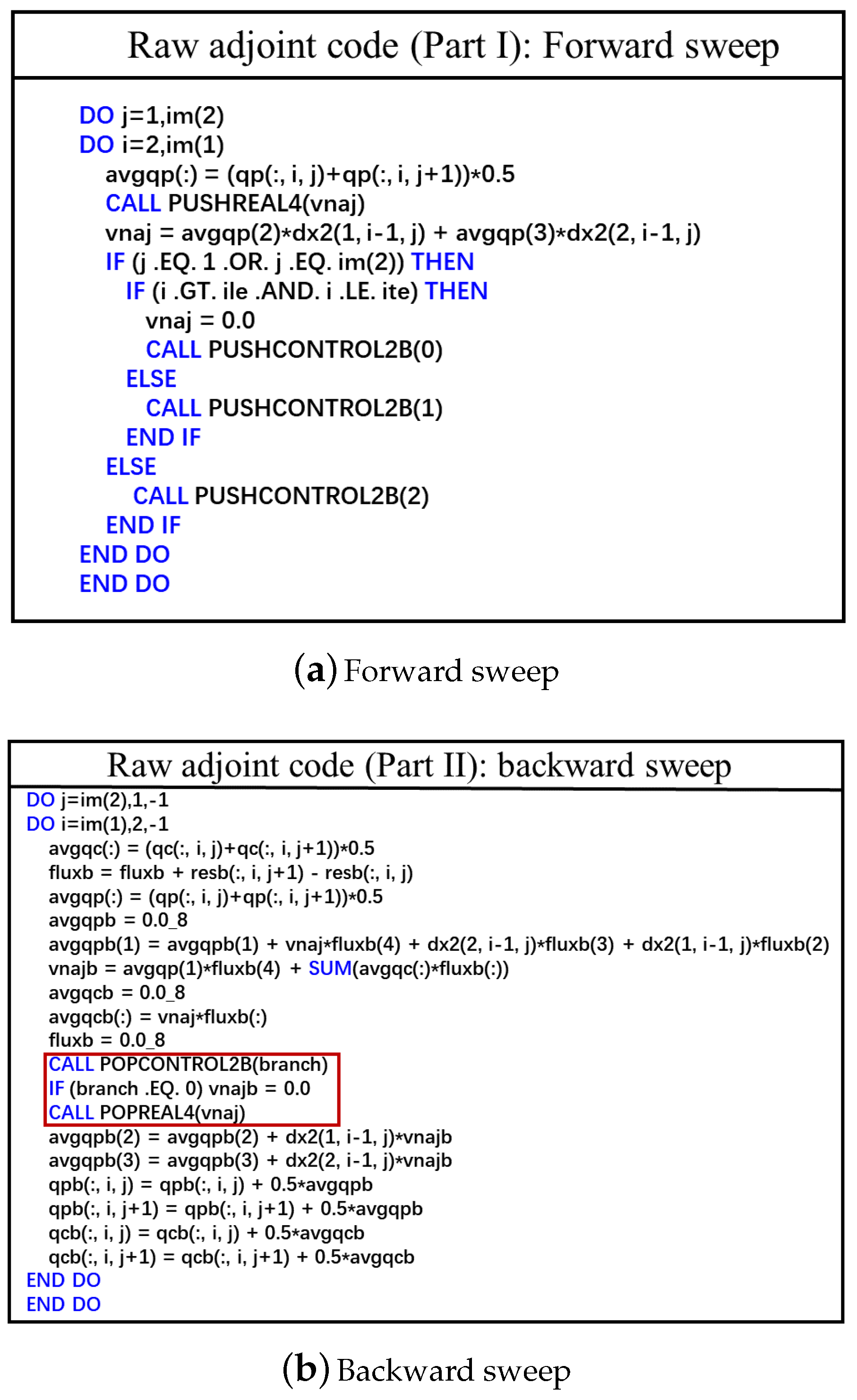
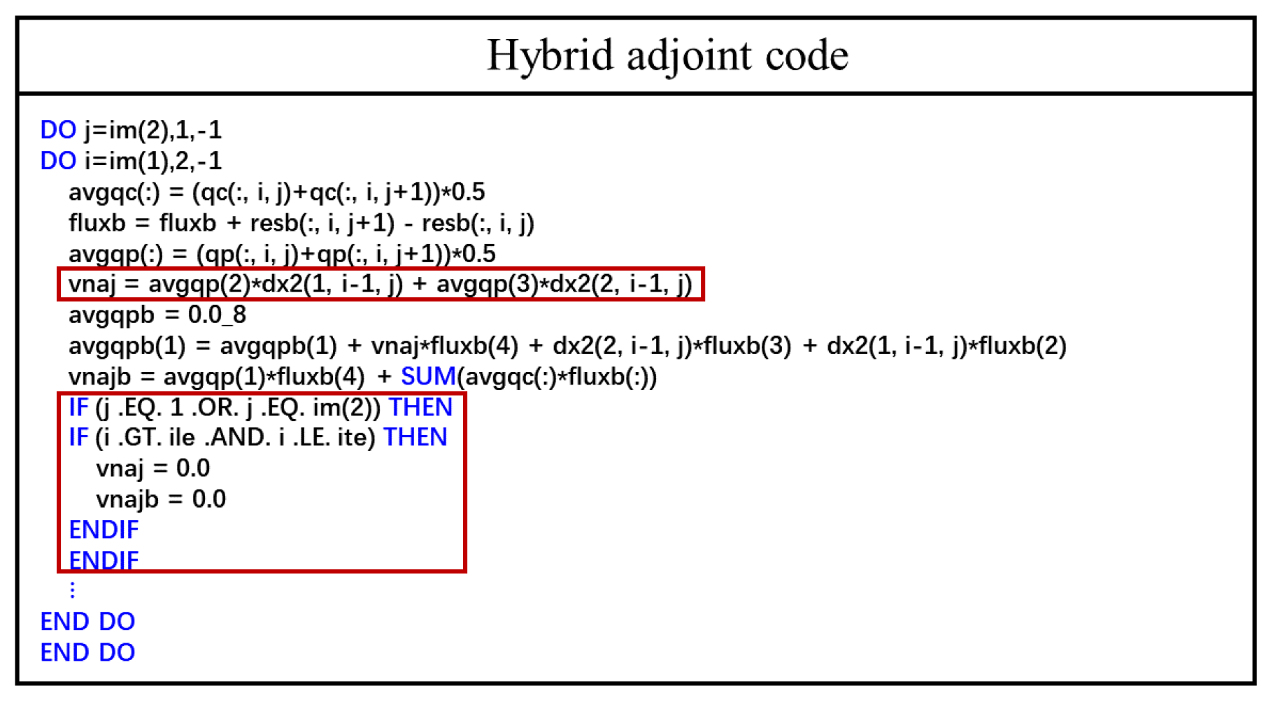
Figure 5 shows part of the codes of a two-dimensional flow solver. The code snippets correspond to the convective flux calculation. In Figure 5, q c is the conservative variable vector; q p is the primitive variable vector; r e s is the spatial residual vector of the flow governing equation; i m ( 1 ) and i m ( 2 ) are the number of grid points in the two grid directions, respectively; d x 2 is the geometry metrics vector of the mesh; and the remaining are intermediate variables. The adjoint codes produced by the AD tool are presented in Figure 6. It contains two parts: the forward sweep part (Figure 6a) and the backward sweep part (Figure 6b). The forward part mainly calculates and stores intermediate variables. The values of the intermediate variables are retrieved in the backward part. Because the flow codes contain different types of intermediate variables, both PUSHCONTROL2B/POPCONTROL2B and PUSHREAL4/POPREAL4 function pairs are called in the raw adjoint codes. The former is for conditional branches, and the latter is for the intermediate variable v n a j . It can be found in the two figures that the number of PUSH/POP function calls required depends on the number of grid points. For cases with millions or even billions of grid points, the function calls will greatly affect the computational efficiency of the adjoint codes.
The strategies used to develop the hybrid adjoint codes are: first, delete the forward part of the adjoint codes (Figure 6a); second, replace the adjoint codes in the red rectangle of Figure 6b with manual codes in the two red rectangles of Figure 7. The manual codes in the first rectangle are used to calculate v n a j and those in the second one are related to the conditional branches. Since the calculation of v n a j b involves v n a j , the manual codes in the first rectangle should be put before v n a j b . Compared with the raw adjoint codes, the hybrid adjoint codes are easier to read. In terms of computational cost, the hybrid adjoint codes are more efficient. This is because there are no PUSH/POP function calls in the hybrid adjoint codes anymore.

6. Rotor-Stator/Stator-Rotor Interface Treatment

6.1. Mixing Plane Method

For multi-row cases, there is a need to exchange solution information during a solution process at the rotor-stator/stator-rotor interface, as shown in Figure 8. In this work, the conservative, robust and non-reflective mixing plane method proposed by Wang [28] is used to realize data exchange. This mixing plane method involves three main steps:
(1)
Average flux in the circumferential direction. It can be expressed in the following symbolic form
( F 0 j ) = f 1 ( U j , X j ) ( j = 1 , 2 )
In Equation (11), the superscript j represents the upstream or downstream of a rotor-stator/stator-rotor interface. When j equals 1, it represents the upstream of the interface, otherwise, it represents the downstream of the interface. The subscript 0 represents the value before flux interpolation. X is the grid coordinate vector, and f 1 is the function related to flux averaging.
(2)
Interpolate flux in the radial direction. This step is a must as the grid distribution in the radial direction across an interface is often different as shown in Figure 8b. The interpolation operation is represented symbolically as follows
R o w 1 : ( F 1 1 ) = f 2 ( X 1 , X 2 , F 0 2 )
R o w 2 : ( F 1 2 ) = f 2 ( X 2 , X 1 , F 0 1 )
where f 2 represents the function related to flux interpolation and subscript 1 represents the interpolated flux.
(3)
Update solution based upon the one-dimensional non-reflective boundary condition. This operation is represented as follows
R o w 1 : ( U 1 , ) = f 3 ( U 1 , F 0 1 , F 1 1 )
R o w 2 : ( U 2 , ) = f 3 ( U 2 , F 0 2 , F 1 2 )
In the above equation, the superscript ∗ represents the updated solution, and f 3 represents the function related to the solution update.
Figure 8. The blade-to-blade and meridional views of an interface.
Aerospace 10 00106 g008

6.2. Discrete Adjoint Mixing Plane Method

Due to the reverse mode of the AD, the three steps will be reversed for the development of the discrete adjoint mixing plane method.
(1)
Differentiate the subroutines related to solution update.
R o w 1 : ( U a 1 , F 0 , a 1 , F 1 , a 1 ) = f 3 _ a ( U 1 , U 1 , , U a 1 , , F 0 1 , F 1 1 )
R o w 2 : ( U a 2 , F 0 , a 2 , F 1 , a 2 ) = f 3 _ a ( U 2 , U 2 , , U a 2 , , F 0 2 , F 1 2 )
where
U a j = ( f 3 U j ) T U a j , ( j = 1 , 2 ) F 0 , a j = ( f 3 F 0 j ) T U a j , ( j = 1 , 2 ) F 1 , a j = ( f 3 F 1 j ) T U a j , ( j = 1 , 2 )
In the above equations, U a 1 , and U a 2 , are initialized by 0.
(2)
Differentiate the subroutines related to flux interpolation.
R o w 1 : ( F 0 , a 2 ) = f 2 _ a ( X 1 , X 2 , F 0 2 , F 1 1 , F 1 , a 1 )
R o w 2 : ( F 0 , a 1 ) = f 2 _ a ( X 2 , X 1 , F 0 1 , F 1 2 , F 1 , a 2 )
where
F 0 , a 2 = F 0 , a 2 + ( f 2 F 1 1 ) T F 1 , a 1 F 0 , a 1 = F 0 , a 1 + ( f 2 F 1 2 ) T F 1 , a 2
(3)
Differentiate the subroutines related to flux averaging.
( U a j ) = f 1 _ a ( U j , X j , F 0 j , F 0 , a j ) ( j = 1 , 2 )
where
U a j = U a j + ( f 1 F 0 j ) T F 0 , a j ( j = 1 , 2 )
In the above equations, the subscript a represents the backward mode of the AD.

7. Results

In this section, the single-stage transonic compressor–NASA Stage 35 [26] and the 1.5-stage Aachen turbine [27]—are used to demonstrate the effectiveness of the multi-row adjoint solver developed by the proposed hybrid automatic and manual approach.

7.1. NASA Stage 35

NASA Stage 35, designed by the NASA Lewis Research Center, is the inlet stage of an advanced-core compressor. It has 36 rotor blades and 46 stator blades with the aspect ratios being 1.19 and 1.26, respectively. At design speed, the peak stage efficiency is 0.872, and the corresponding stage total pressure ratio is 1.842. More detailed design parameters of the stage can be found in reference [26].

7.1.1. Grid Independence Study

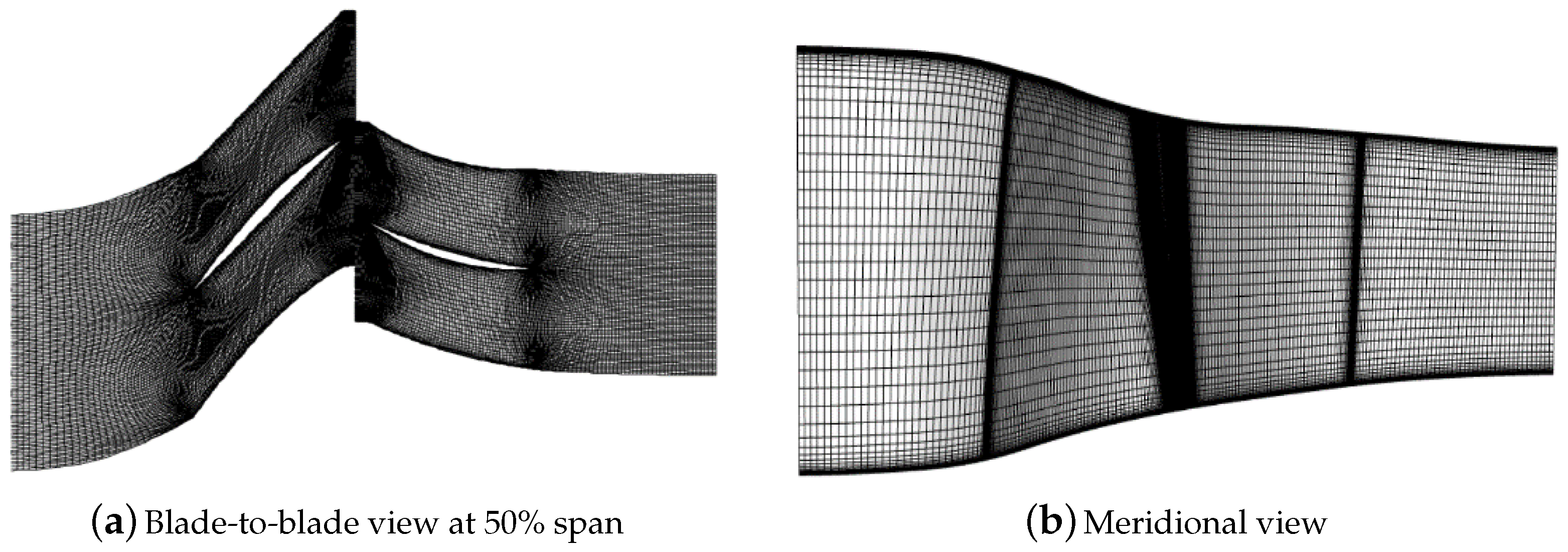
First, the grid independence study following the procedure introduced in reference [32] is performed to find a grid-converged solution. Three different grids–Grid1, Grid2, and Grid3—are used. Table 1 shows the allocation of grid nodes in the three coordinate directions. The number of grid nodes is successively increased by a factor of 2 from Grid1 to Grid3. Figure 9 shows the blade-to-blade and meridional views of Grid2.
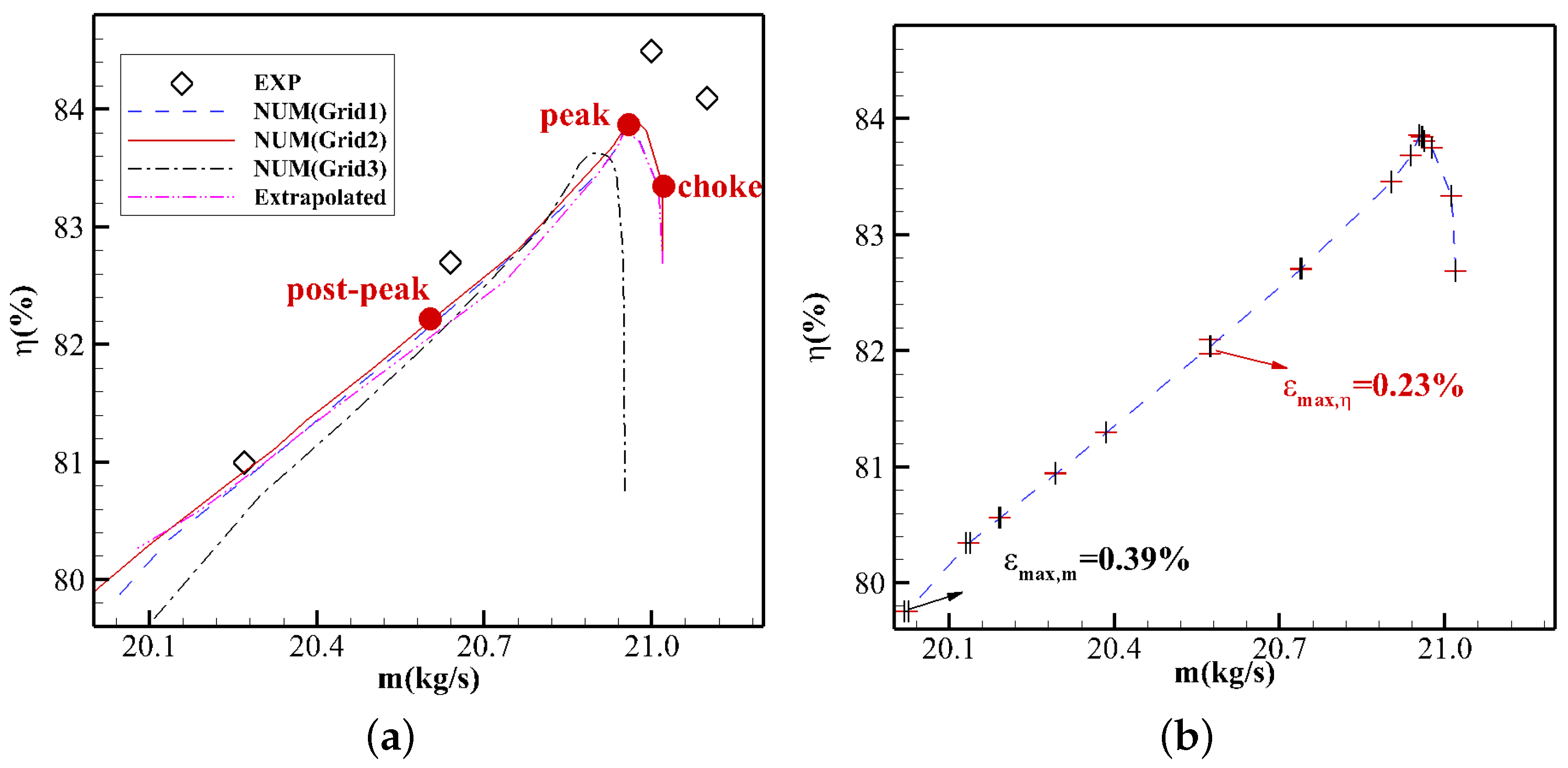
Two aerodynamic metrics-isentropic efficiency ( η ) and total pressure ratio ( π ) are taken into account. Figure 10a presents the isentropic efficiency against the mass flow rate at 100% design speed. In the legend, EXP represents the experimental data, and Extrapolated represents the extrapolated solution using the equations in reference [32]. The extrapolated solution is used to compute the error bars in Figure 10b. It can be seen in Figure 10a that the numerical solution from Grid2 agrees well with that from Grid1. However, there is a big difference between Grid3 and the other two numerical solutions, especially close to the choke point. Figure 10b presents the fine-grid solution and the corresponding discretization error bars. The maximum discretization uncertainty of isentropic efficiency ( ϵ m a s s , η ) is 0.23%, which corresponds to ± 0.19 .
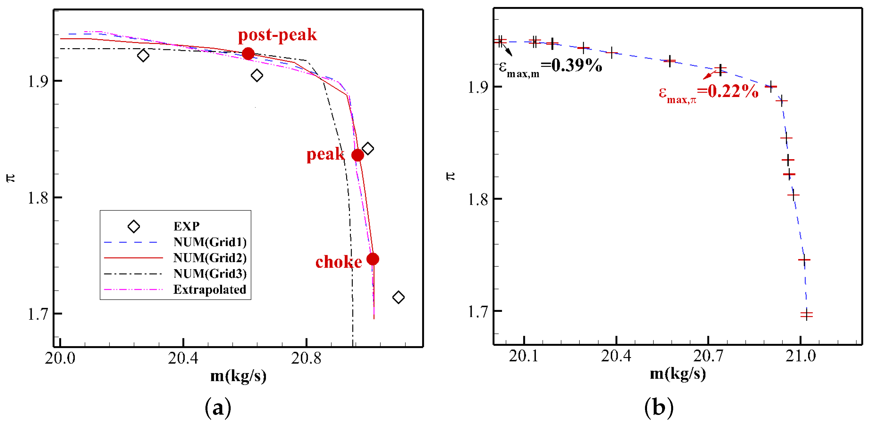
In terms of total pressure ratio and mass flow rate (see Figure 11a,b), the maximum discretization uncertainties of total pressure ratio and mass flow rate are 0.22% ( ϵ m a s s , π ) and 0.39% ( ϵ m a s s , m ), which corresponds to ± 0.0042 and ± 0.08 kg/s, respectively. Based on the above results, it is concluded that the discretization uncertainties are very small and a grid-converged solution is obtained. To make a trade-off between solution accuracy and computational cost, Grid2 will be selected in our study.

7.1.2. Adjoint Sensitivity Verification

The adjoint sensitivities are verified by the multi-row linearized solver developed by the forward mode of the AD tool. According to the duality property, the adjoint solver should have the same sensitivity convergence history as the corresponding linearized solver.
In this investigation, the objective function is isentropic efficiency, and the design variables are inlet total temperature (T0) and inlet total pressure (P0). The use of inlet total temperature and pressure as design variables for sensitivity verification does not involve mesh deformation and thus avoids associated complications. Figure 12 shows the turbulence variable contours and the adjoint variable contours corresponding to the turbulence model equation at 50% span. It can be seen that the upstream of the adjoint fields corresponds to the downstream of the flow fields and vice versa. This feature can be used to qualitatively verify the correct development of the multi-row discrete adjoint solver.
The sensitivity convergence histories from the linearized and adjoint solvers are presented in Figure 13. In the legend, LIN represents the linearized solver, CEV represents the adjoint solver with the CEV assumption, and hybrid ADJ represents the full viscosity adjoint solver developed by the hybrid automatic and manual differentiation. It can be seen in the two figures that the sensitivity convergence histories from the linearized solver almost overlap with those from the hybrid ADJ. The relative difference in sensitivity is no more than 0.3%. However, the CEV assumption has an adverse effect on the sensitivity accuracy, especially for the design variable of the inlet total temperature. Over 50% relative difference of sensitivity between LIN and CEV can be observed in Figure 13b.
In this part, the sensitivities of isentropic efficiency and mass flow rate to geometric design variables are verified. In this study, the Hicks-Henne hump functions [33] are used to parameterize perturbations to a blade camber. Accordingly, the design variables are the coefficients of Hicks-Henne functions. Fifteen design variables from the first row and twelve design variables from the second row are randomly selected from different spans and chord-wise positions. Sensitivities from the finite difference method (FDM) with a constant step size of 10 4 are used as references. Figure 14 presents the sensitivities computed by three different methods. It can be seen that the sensitivities from the hybrid ADJ agree well with those from the FDM. The maximum relative difference is no more than 1%, which is acceptable for engineering design optimizations. However, the CEV assumption harms sensitivity accuracy, especially for the design variables of the rotor blade camber. In summary, the sensitivities obtained using the hybrid ADJ are reliable, and the CEV assumption has a markedly adverse effect on sensitivity accuracy.

7.1.3. Computational Efficiency

In this part, the computational efficiency of the original adjoint solver without manual adaption, the hybrid adjoint solver, and the flow solver will be compared. The solvers are run on an Intel Xeon Gold 6233 CPU @ 2.50 GHz workstation. When different solvers are run, the workload of the workstation is kept identical to ensure a fair comparison. Figure 15a presents the root mean square (RMS) residual convergence histories of both the flow and adjoint solvers. In the legend, original ADJ represents the discrete adjoint solver developed by using the AD tool without manual adaption. With the increase in iterations, both the flow and adjoint solvers’ RMS residual curves go down. After 10,000 iterations, the flow solution is fully converged. From Figure 13, it is also known that 10,000 iterations are also enough to obtain converged adjoint sensitivities. The other point found is that the hybrid adjoint solver has the same residual convergence as the original adjoint solver. This means that the manual adaption does not affect the residual convergence. Figure 15b makes a comparison in CPU time among different solvers when 10,000 iterations are finished. It can be seen that both adjoint solvers consume more CPU time than the flow solver. However, compared with the original ADJ, the hybrid ADJ is more efficient. About 43% time can be saved. Moreover, 9% of memory can also be saved by the hybrid ADJ. The detailed comparison of time and memory consumption among different solvers can be found in Table 2.

7.1.4. Results of Design Optimizations

The multi-row turbomachinery aerodynamic design optimization is performed using the hybrid ADJ. To improve the aerodynamic performances over the whole 100% design speed, three operating points–the peak, a choke, and post-peak points—are selected (as marked in Figure 10a and Figure 11a). The isentropic efficiency at the three operating points is weighted to form a single objective function. Moreover, to constrain the mass flow rate and total pressure ratio at different operating points, they are transferred into the objective function by the penalty function method. The single objective function can be expressed by
I = j ω j I j ( j = s , c , p )
I j = η j , 0 η j + σ m ( m j m j , 0 1 ) 2 + σ π ( π j π j , 0 1 ) 2
where σ m and σ π are penalty coefficients of mass flow rate and total pressure ratio and set to 200; the subscript 0 represents the initial value and the weighting coefficients are set to 0.25 for both the post-peak efficiency point (s) and the choke point (c) and 0.5 for the peak efficiency point (p).
The blade camber perturbation is parameterized in this optimization using the Hicks-Henne hump functions. For each row, the blade cambers at seven spans—10%, 20%, 35%, 50%, 65%, 80%, and 90% are extracted. Fifteen design variables for the first row and twelve design variables for the second row are uniformly distributed along a blade camber, leading to 189 design variables in total. The steepest descent method with a constant step size of 1.0 × 10 6 is used to update design variables and thus blade profiles.
The evolution histories of the objective functions and constraints are presented in Figure 16. After 11 design cycles, the weighted objective function is decreased by 0.6%, and the weighted mass flow rate and total pressure ratio variations are negligible. A detailed comparison of aerodynamic performances can be found in Table 3. Optimization significantly improves the isentropic efficiency at all three operating points. Figure 17a,b compare the isentropic efficiency and total pressure ratio against the mass flow rate between the original and optimized blade profiles at the 100% design speed. It can be seen that the isentropic efficiency is improved, and the total pressure ratio is maintained over the entire operating range of 100% speed. Furthermore, the stall mass flow rate decreases after optimization, leading to an improved stall margin.
Figure 18 compares original and optimized blade profiles at three different spans—10%, 50%, and 90%. The major geometry change occurs to the stator blade from the hub to the mid-span. There is also a change to the rotor blade with the most change occurring below the mid-span.
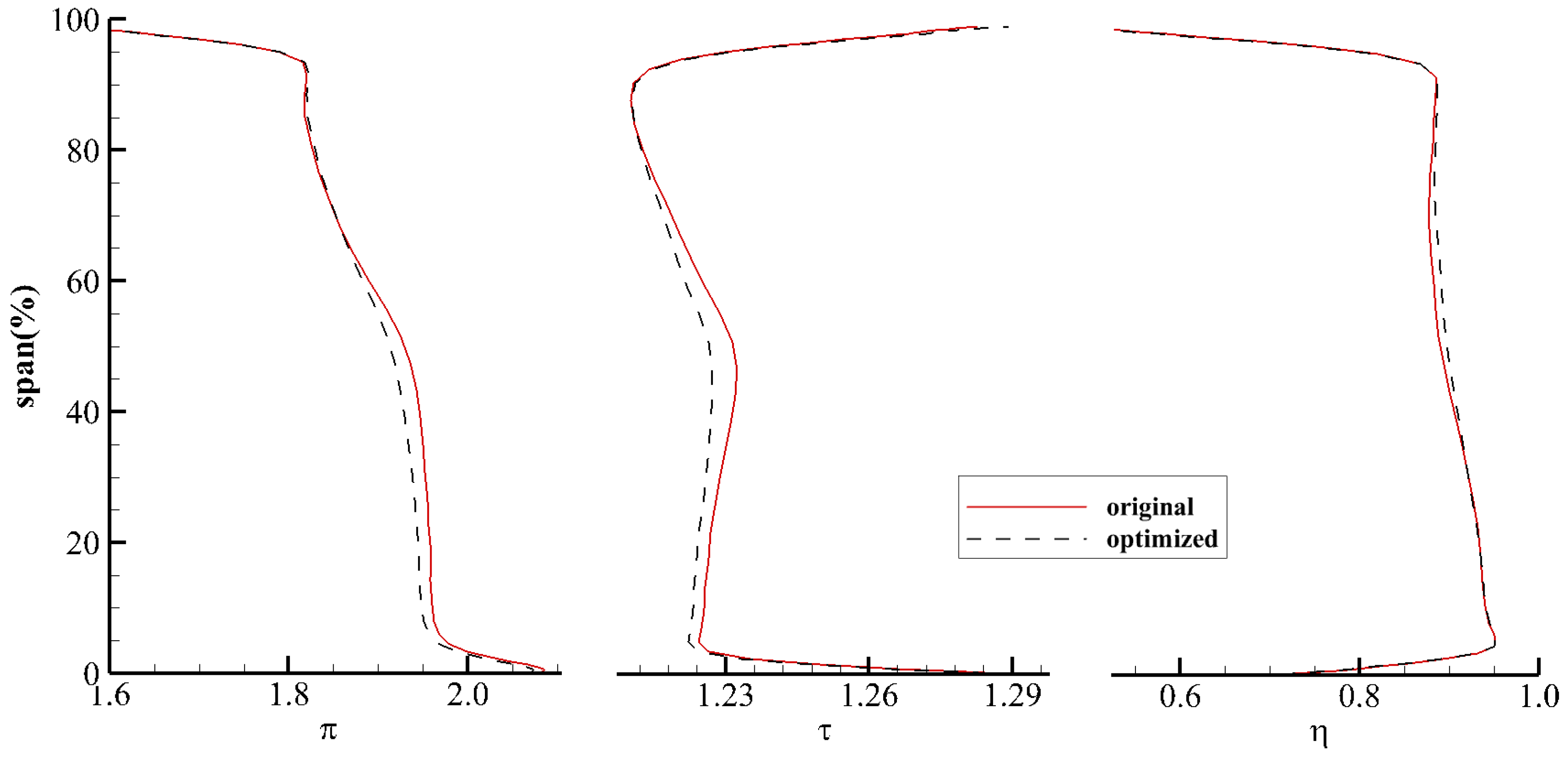
The rotor blade camber decreases from the leading edge to the middle chord and increases slightly over the remaining chord. This reduces the blade loading, leading to reduced flow separation region on the suction surface after the shock (see Figure 19). The radial distributions of the rotor aerodynamic parameters, as shown in Figure 20, further demonstrate this point. In Figure 20, the performance metrics are calculated along a streamwise grid line. The metrics do not necessarily represent the actual performance of the local flow field, as the flow often does not follow a grid line. Nevertheless, the metrics can still reveal the performance variations between the original and the optimized designs, as the mesh at the inlet and the outlet of a domain will not change after optimization. It can be seen in Figure 20 that the total temperature and pressure ratios, except for the blade tip region, decrease after optimization. An increase in the isentropic efficiency, especially from the 40% span to the 70% span, can be observed.
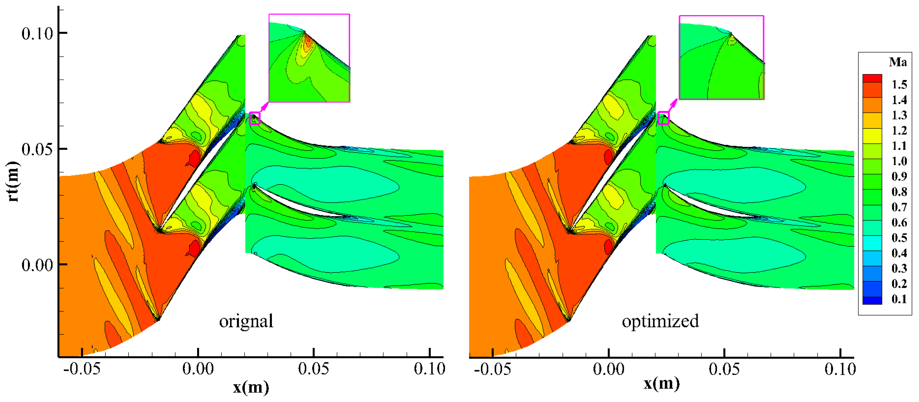
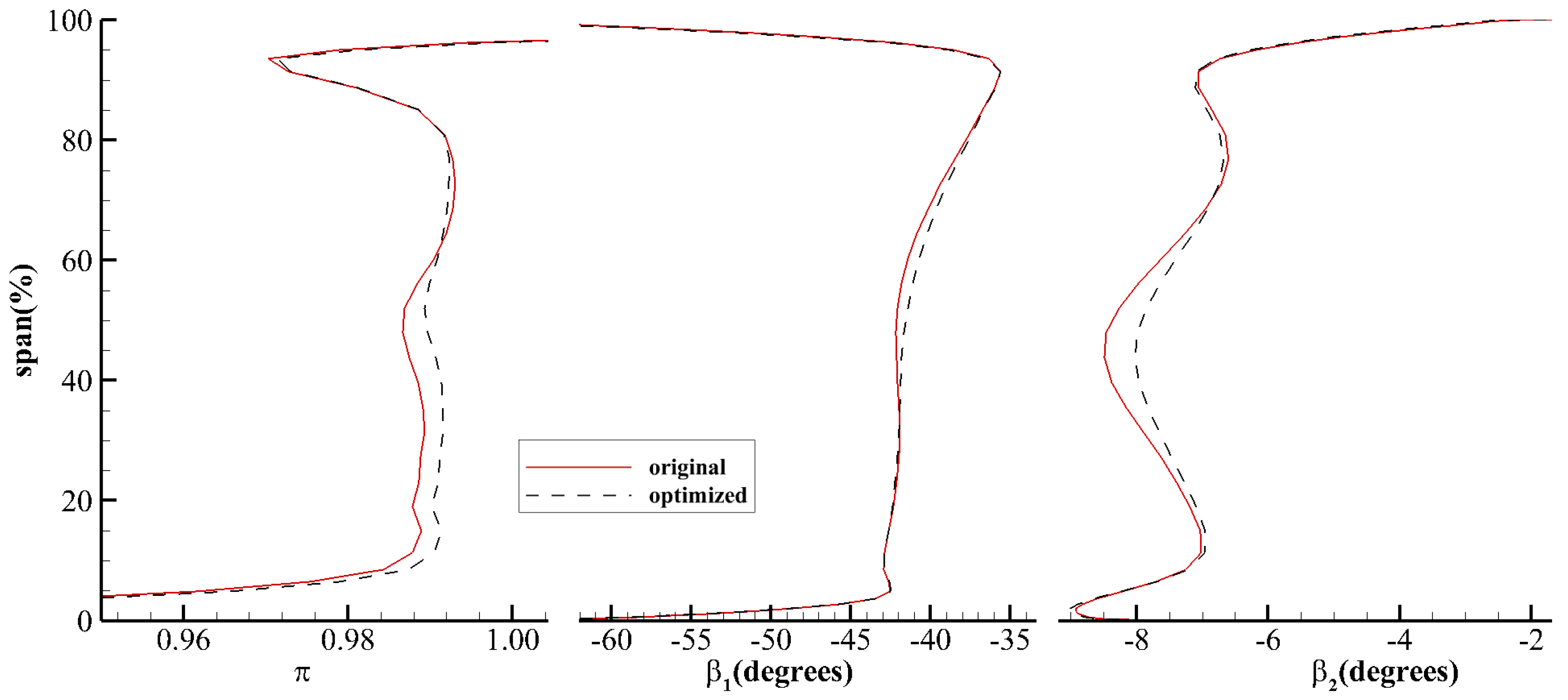
The stator blade camber is increased over the whole chord. This reduces the local incidence, leading to reduced profile loss. The reduced incidence also reduces the supersonic patch and associated aerodynamic loss on the blade suction side as shown in the close-up of Figure 19. Figure 21 compares the radial distributions of the stator aerodynamic parameters-total pressure ratio, inlet, and outlet flow angle ( β 1 and β 2 ), calculated across the stator only. The total pressure ratio is greatly increased from the hub to the 60% span and slightly decreased from the 60% span to the 80% span. Overall, the total pressure ratio increases for the optimized blade profiles. The inlet flow angle (absolute value) reduces from the 30% span to the 80% span. The reduced flow angle together with the increased blade inlet angle further reduces the incidence and profile loss. The outlet flow angle increases from the 10% span to the 70%, however, a slight increase can be observed from the 70% span to the 90% span. Around the hub and shroud, there is no visible difference between the original and optimized blade profiles.

7.2. Aachen Turbine

The second case used herein to demonstrate the effectiveness of the hybrid adjoint solver developed in our work is the 1.5-stage Aachen turbine. The blade counts in each row are 36, 41, and 36, respectively. The rotation speed of the rotor blade is 3500 rpm.
Figure 22a presents the three-dimensional mesh and Figure 22b presents the blade-to-blade view of the mesh at 50% span. The mesh has a density of 149 ( a x i a l ) × 57 ( c i r c u m f e r e n t i a l ) × 57 ( r a d i a l ) in the first row, 133 ( a x i a l ) × 61 ( c i r c u m f e r e n t i a l ) × 73 ( r a d i a l ) in the second row, and 141 ( a x i a l ) × 57 ( c i r c u m f e r e n t i a l ) × 57 ( r a d i a l ) in the third row, leading to 1.53 million grid nodes in total.

7.2.1. Adjoint Sensitivity Verification

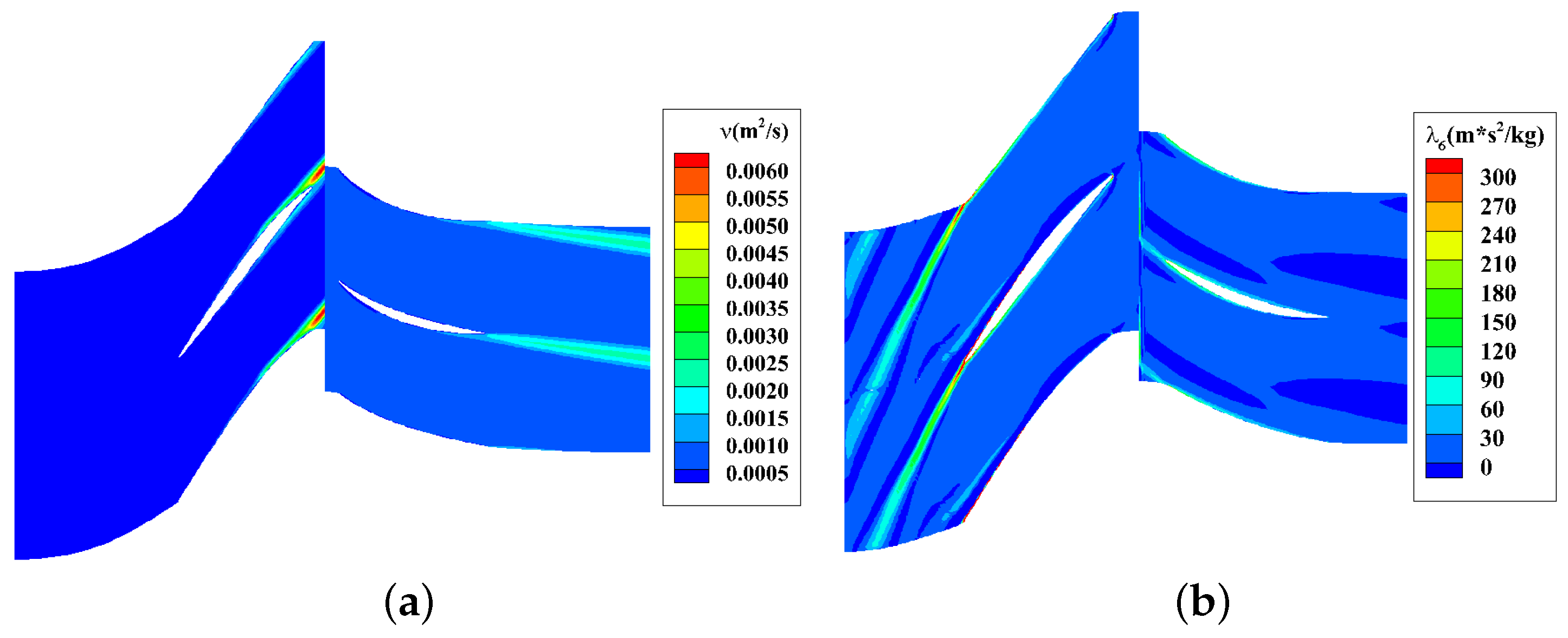
Similar to the NASA Stage 35, two kinds of design variables are considered in the sensitivity verification part. The first type is the inlet boundary condition including the inlet total pressure and the inlet total temperature, and the second type is the coefficients of Hicks-Henne hump functions. The objective functions taken into account are the mass flow rate and the entropy generation rate. Figure 23a shows the turbulence variable contours, and Figure 23b shows the adjoint variable contours corresponding to the turbulence model equation at 50% span. It can be seen that the upstream and downstream of the adjoint fields are also opposite to those of the flow fields. This feature qualitatively verifies the correct development of the multi-row discrete adjoint solver.
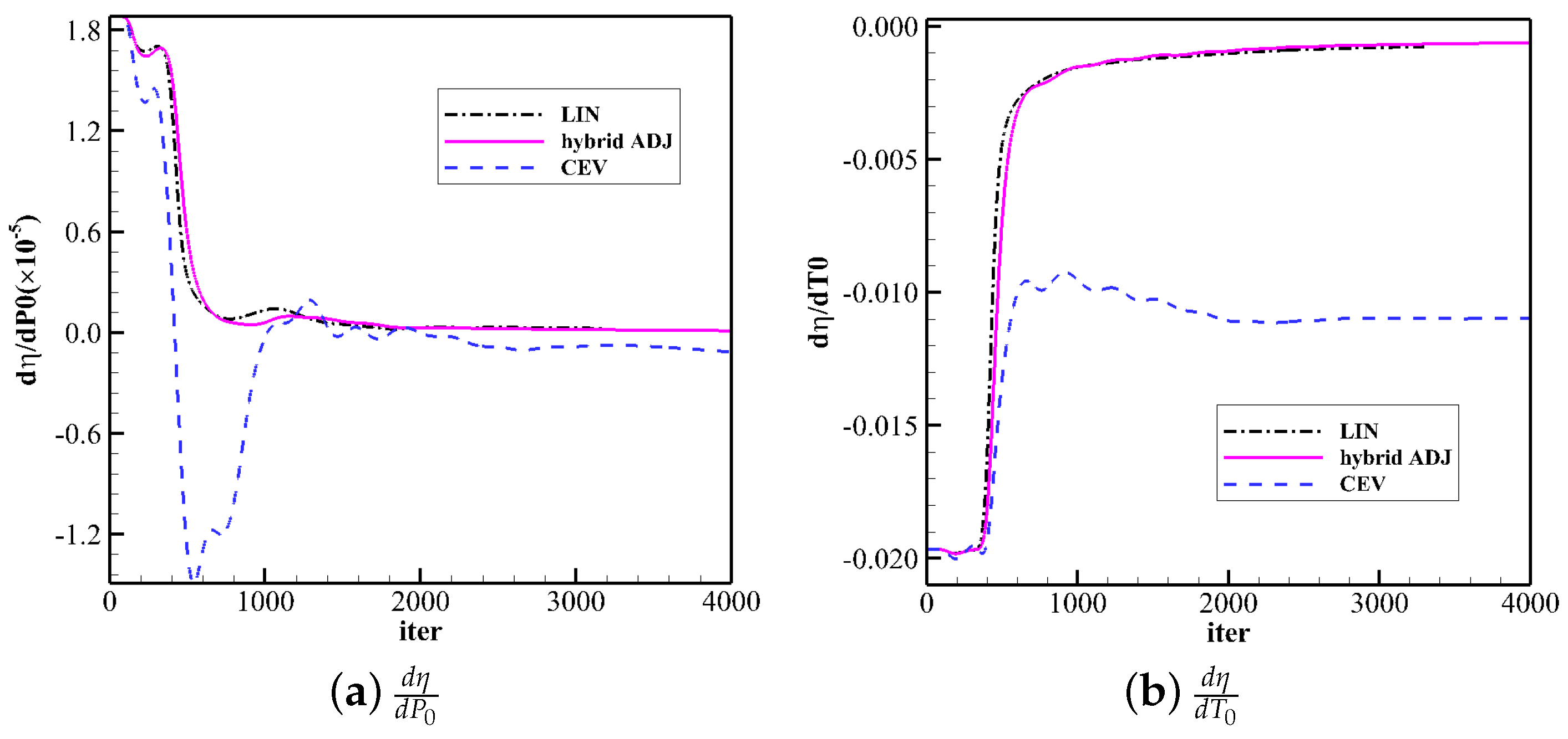
Figure 24a,b present the sensitivity convergence histories of the entropy generation rate to the inlet total pressure and the inlet total temperature, respectively. It can be seen in the two figures that the hybrid ADJ almost has the same sensitivity convergence histories as the LIN, while there is a visible difference between the CEV and the hybrid ADJ, especially for the design variable of the inlet total pressure. Compared with NASA Stage 35, the effect of the CEV assumption on sensitivity is smaller, and the maximum difference for the design variable of the inlet total pressure is less than 20%.
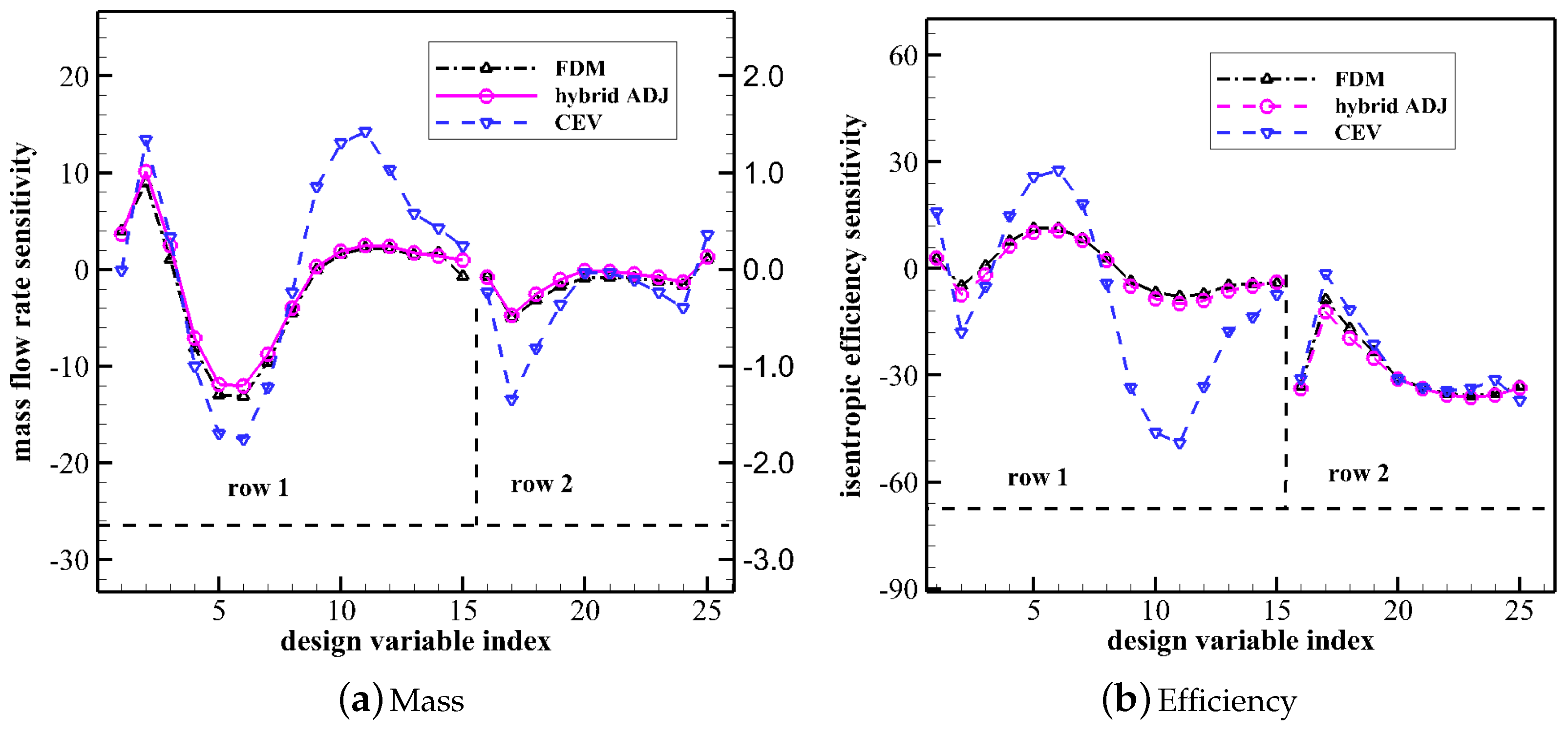
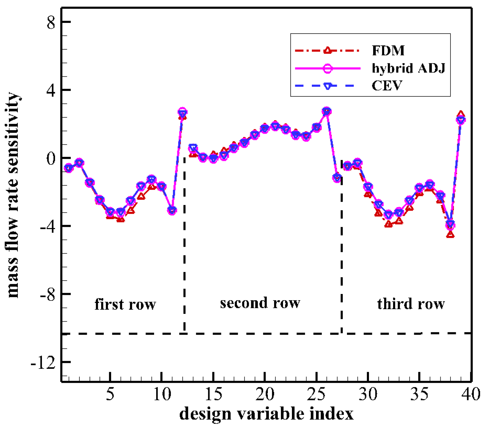
Figure 25 compares the sensitivity accuracy among different methods with the coefficients of the Hicks-Henne hump function being used as design variables. Twelve design variables for both s0 and s1 and fifteen design variables for r1 are randomly selected from different spans and chords in this verification. There is good agreement in sensitivities between the hybrid ADJ and the FDM. The maximum relative difference comes from s1 but is still small enough (less than 1.0%). Different from NASA Stage 35, the effect of the CEV assumption on the sensitivity accuracy of the Aachen turbine is not obvious. The CEV sensitivities also have good agreement with the FDM sensitivities.

7.2.2. Computational Efficiency

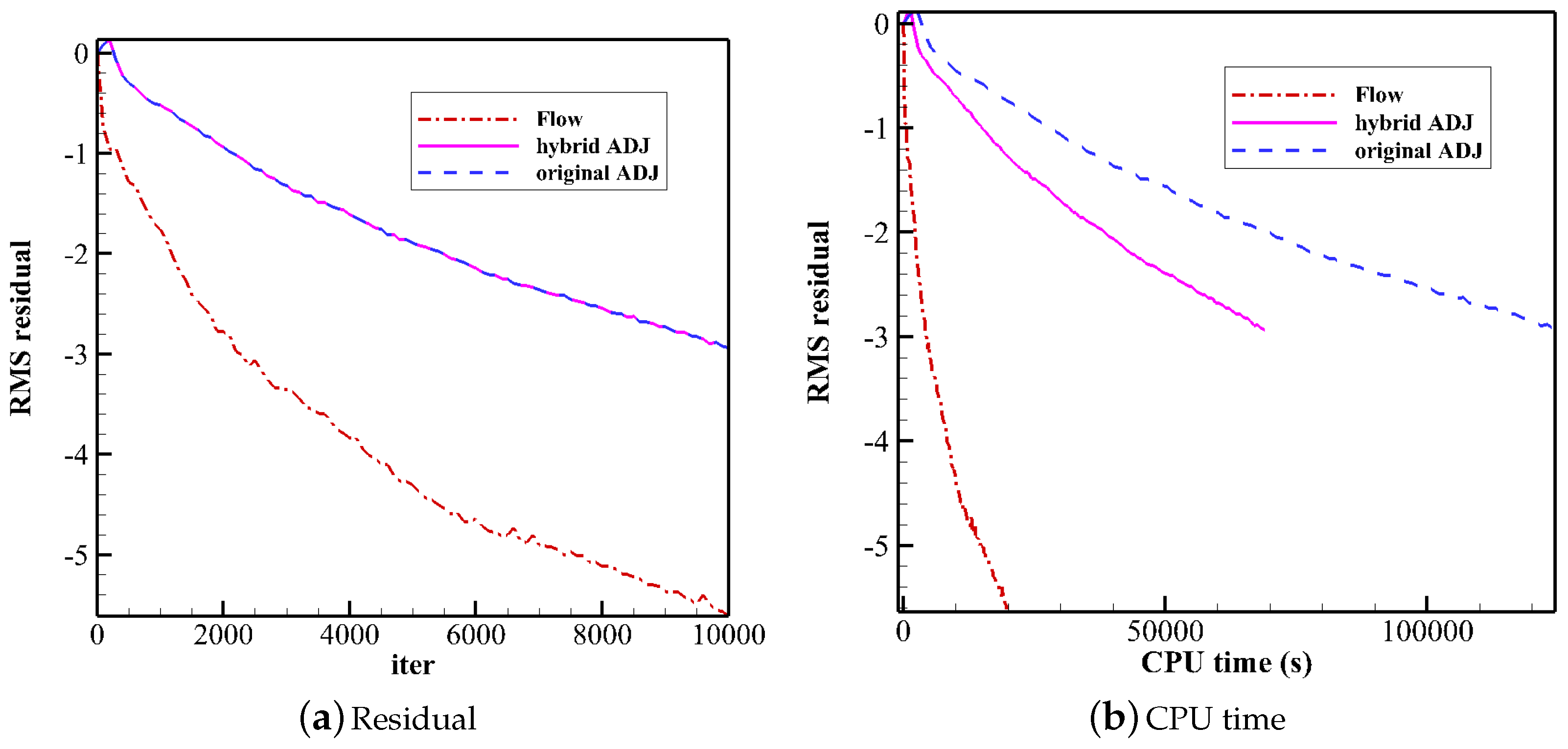
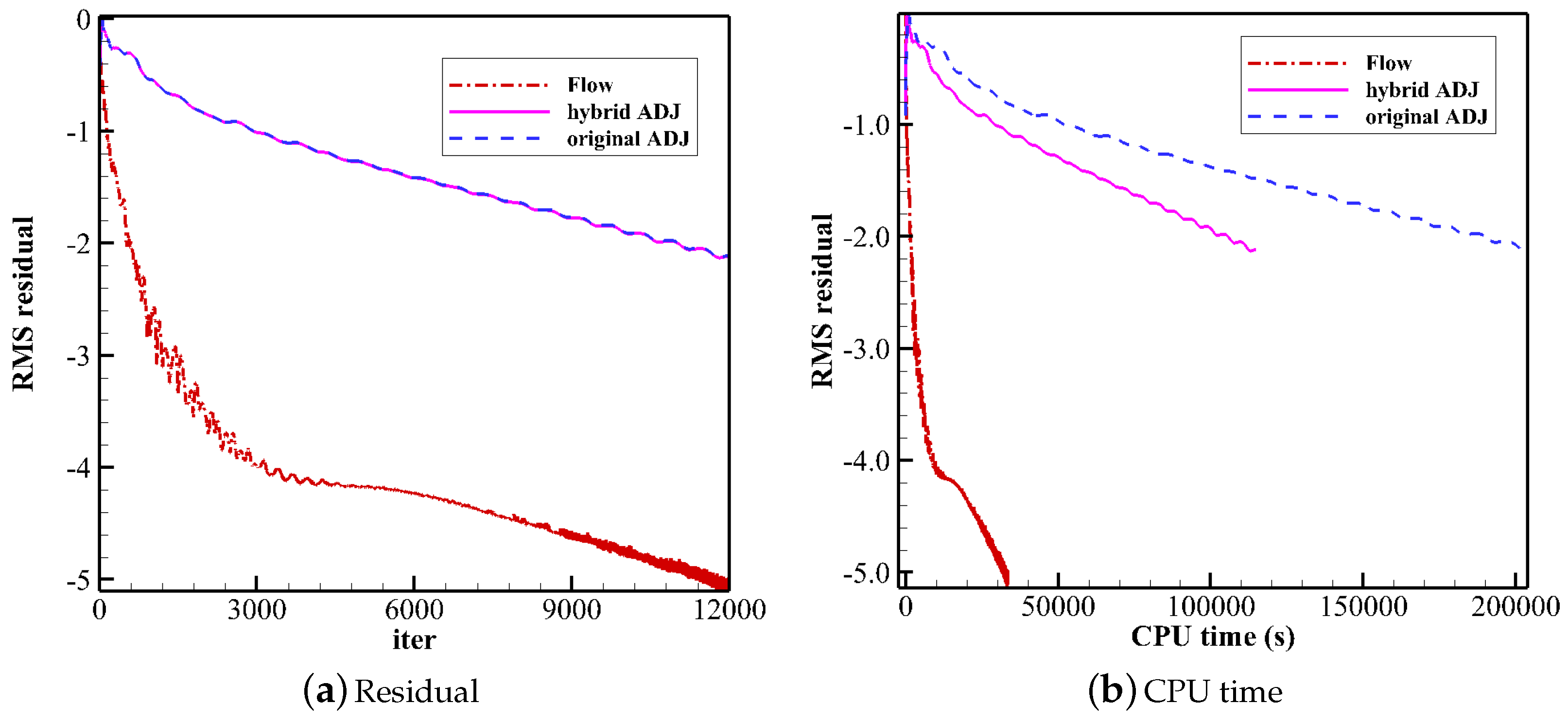
Figure 26a shows the RMS residual convergence histories of the flow and adjoint solvers. It can be seen in this figure that after 12,000 iterations, the flow solution is converged. Moreover, the adjoint RMS residual reduces by over two orders, which is enough to obtain converged adjoint sensitivities (see Figure 24).
To verify the high computational efficiency of the hybrid ADJ over the original ADJ, the RMS residual against the CPU time is compared, as shown in Figure 26b. The iterations are set to 12000 for all solvers. Still, both the original and hybrid adjoint solvers consume more time than the flow solver. Compared with the original ADJ, the hybrid ADJ can save 44% CPU time (see Table 4). Moreover, it is found that the hybrid ADJ can save 9.6% of memory (see Table 4).

7.2.3. Results of Design Optimizations

The entropy generation rate can measure the aerodynamic loss within the flow fields. Therefore, the normalized entropy generation rate is used as the objective function in this optimization. To maintain the mass flow rate and total pressure ratio, they are transferred into the objective function by the penalty function method. The weighted objective function is given by
I = d s d s 0 + σ m ( m m 0 1 ) 2 + σ π ( π π 0 1 ) 2
where
d s = s o u t s i n s = ρ [ C p l n ( T t T r e f ) R g l n ( P t P r e f ) ] v · n d S ρ v · n d S
In the above equations, the subscript o u t and i n represent the outlet and inlet of the computational domain; s is the entropy generation rate; ρ is the density; v is the velocity vector; d S is the differential surface area, and n denotes the unit outward normal vector; P t and T t are the total pressure and total temperature; P r e f and T r e f are the reference pressure and temperature and set to 1atm and 288.15 K, respectively; C p and R g are the heat capacity at constant pressure and gas constant; the penalty coefficients of mass flow rate ( σ m ) and total pressure ratio ( σ π ) are set to 200.
The Hicks-Henne hump functions are also used in this optimization to parameterize the blade camber perturbation. Same as the NASA Stage 35, the blade cambers at seven spans are extracted for all rows. In the first and third rows, there are 12 uniformly distributed design variables for each blade section, leading to 84 design variables for each row. In the second row, 15 uniformly distributed design variables for each blade section lead to 105 design variables. The number of design variables in total is 273.
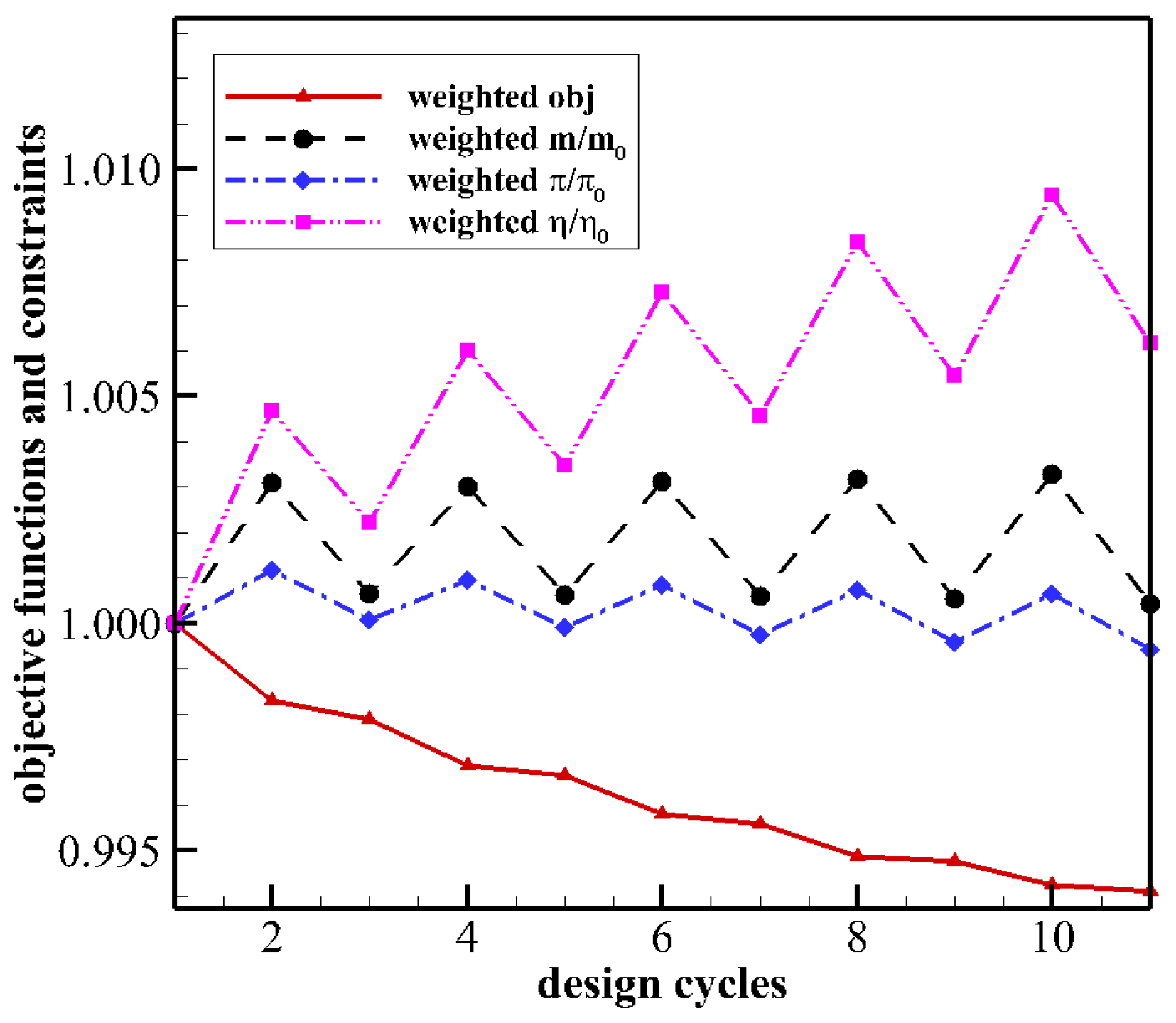
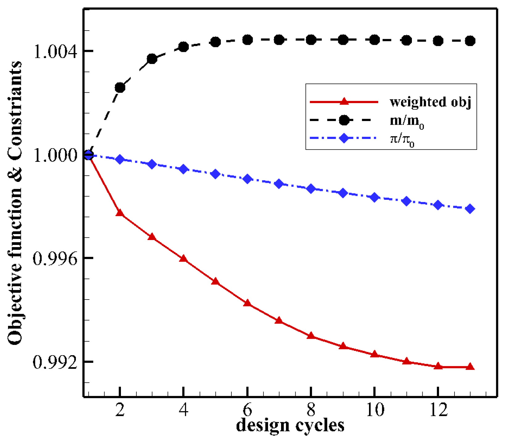
Figure 27 shows the evolution histories of the weighted objective function and constraints. It can be seen in this figure that, after thirteen design cycles, the weighted objective function goes flat and is decreased by 0.8%. The variations in mass flow rate and total pressure ratio are also within an acceptable range.
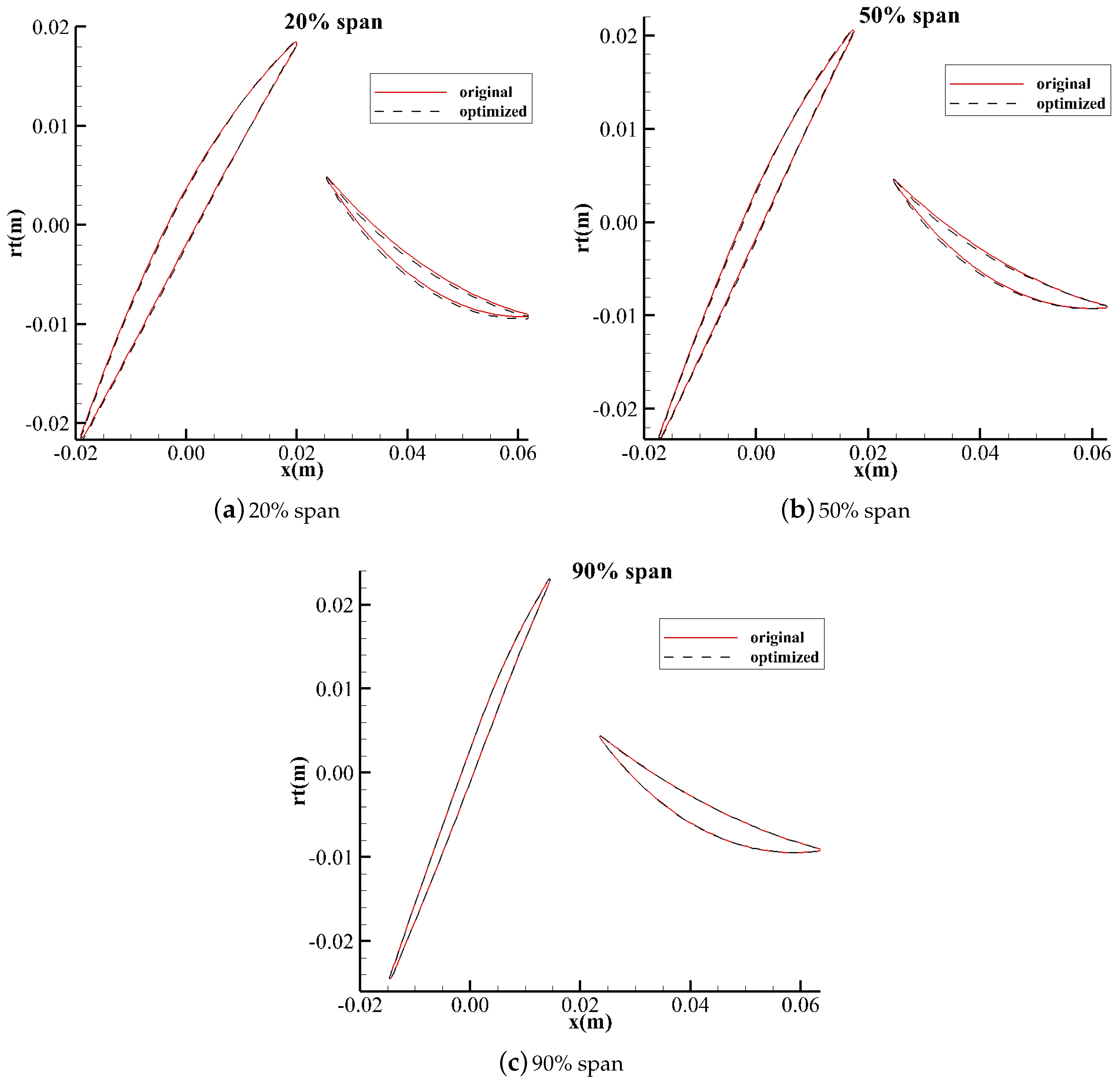
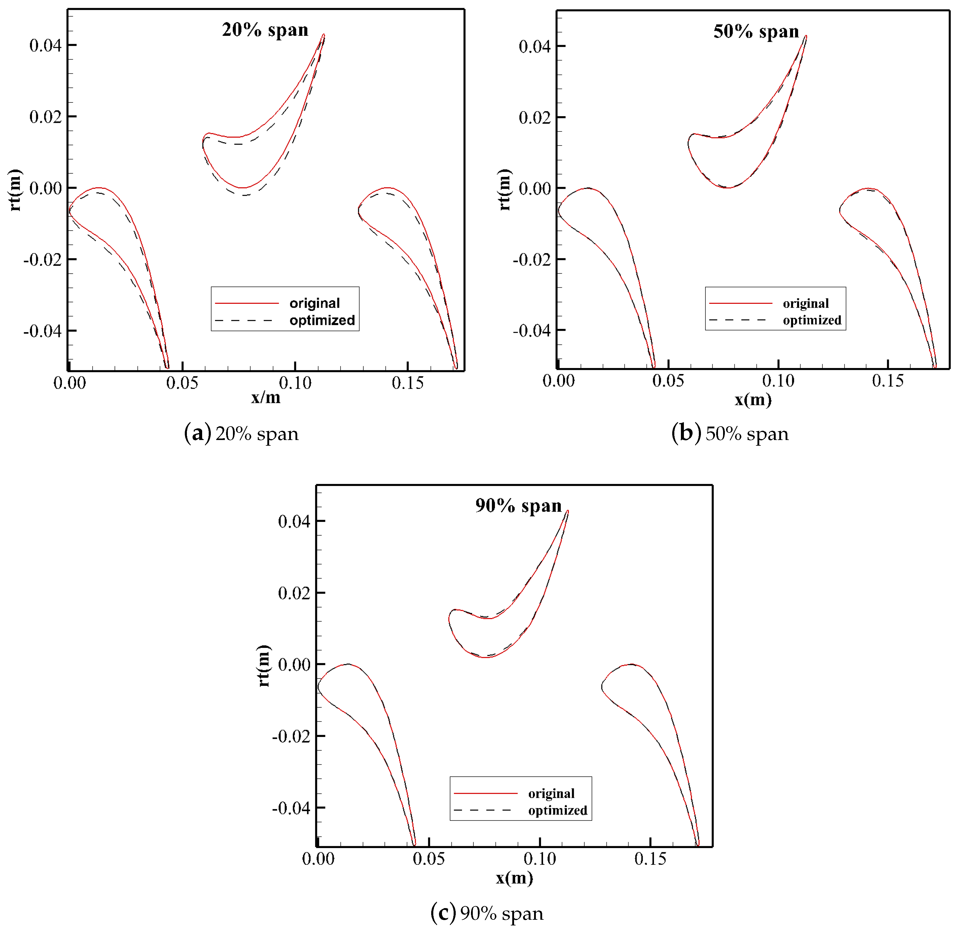
Figure 28 compares the original and optimized blade profiles. All three rows have significant changes in blade profiles near the hub. The changes in blade profiles in the first and third rows are almost consistent: the blade camber is reduced over the whole blade chord. The camber of the second blade row is increased.
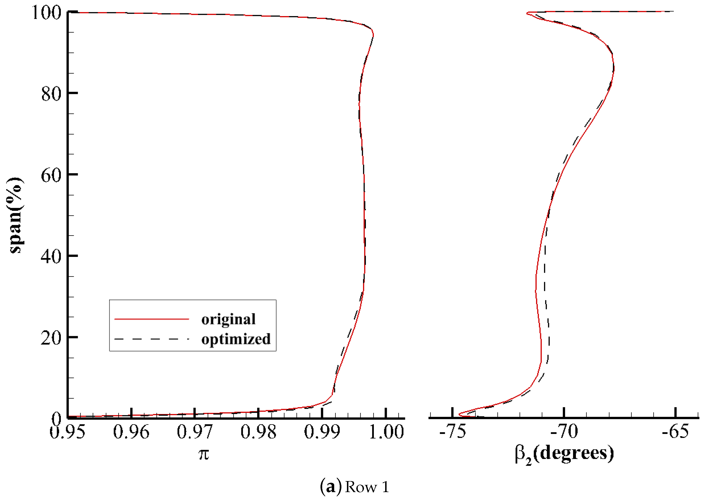
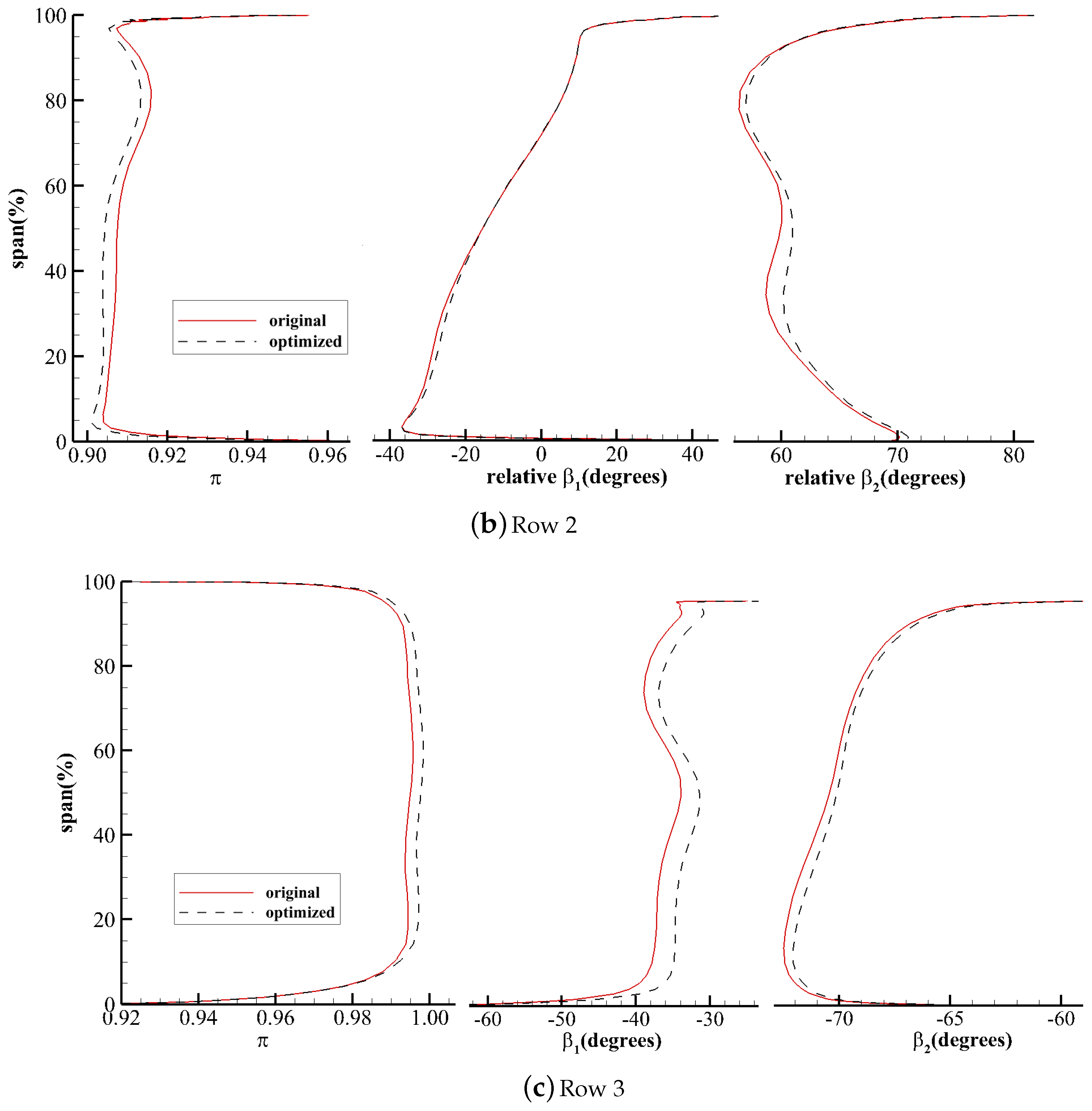
Figure 29a–c compare the radial distributions of aerodynamic parameters of each row. The total pressure ratio and the outlet flow angle are presented in the first row. It can be seen that there is no visible difference in radial distributions of the total pressure ratio along the whole span. The outlet flow angle decreases from the hub to the mid-span and slightly increases from the mid-span to the 80% span while the change in the blade tip region is negligible. The reduced outlet flow angle below the middle span can be explained by the reduced blade camber resulting in a reduced turning angle. In the second row, the optimized total pressure ratio decreases, and the relative turning angle increases (the relative outlet flow angle increases while the relative inlet flow angle is almost maintained) compared with the original one. This is because the rotor blade with an increased camber extracts more energy from its surrounding flows, leading to more pressure drop and a bigger relative turning angle. In the third row, optimization increases the total pressure ratio along the whole span. The increase in total pressure ratio can be attributed to the reduced blade loading resulting from the increased blade inlet angle and the reduced inlet flow angle.

8. Conclusions

This work proposes a hybrid automatic and manual differentiation approach to develop an efficient and accurate discrete adjoint solver. This approach replaces the PUSH/POP function calls in the raw adjoint codes with the manually developed codes. Two strategies for the manual adjustment to the adjoint codes are proposed based on the data types of intermediate variables: directly evaluate conditional branches and compute reals/integrals. For real-life CFD codes, different types of intermediate variables tend to co-exist in the same subroutine, and a combination of the two proposed strategies is required. To demonstrate the effectiveness of the hybrid discrete adjoint solver, the single-stage transonic compressor–NASA stage 35 and the 1.5-stage Aachen turbine—are used. The information exchange at the inter-row interface is achieved by a conservative, non-reflective, and robust mixing plane method for the multi-row flow solver and a discrete adjoint mixing plane method for the multi-row adjoint solver. According to the above results, the following conclusions can be drawn:
(1)
The hybrid ADJ almost has the same sensitivity convergence histories as those from the linearized solver and higher sensitivity accuracy than the CEV. The maximum relative difference of sensitivities between the FDM and the hybrid ADJ is no more than 1.0 % for the cases studied in the paper.
(2)
The hybrid ADJ has higher computational efficiency than the discrete adjoint solver purely developed by the AD tool. About 43 % CPU time and 9.0 % memory consumption can be saved for the single-stage NASA Stage 35, and 44 % CPU time and 9.6 % memory consumption can be saved for the 1.5-stage Aachen turbine.
(3)
The multi-row turbomachinery aerodynamic design optimizations can be effectively performed by the hybrid ADJ. For the single-stage NASA Stage 35, the isentropic efficiency over the entire operating range of 100 % design speed is significantly improved, and the stall margin is increased for the optimized blades. For the 1.5-stage Aachen turbine, the entropy generation rate is decreased after optimization. Moreover, the variations in mass flow rate and total pressure ratio are also acceptable.

Author Contributions

Methodology, H.W.; Software, H.W.; Validation, X.D.; Writing—original draft, H.W.; Writing—review & editing, D.W.; Supervision, D.W.; Funding acquisition, X.H. All authors have read and agreed to the published version of the manuscript.

Funding

This research was supported by the National Science and Technology Major Project (2017-II-0009-0023), China’s 111 project under the grant no. of B17037. This research was also sponsored by the Innovation Foundation for Doctor Dissertation of Northwestern Polytechnical University under the grant no. of CX2022045.

Conflicts of Interest

The authors declare no conflict of interest.

References

  1. Oyama, A.; Liou, M.; Obayashi, S. Transonic Axial-Flow Blade Optimization: Evolutionary Algorithms/Three-Dimensional Navier-Stokes Solver. J. Propuls. Power 2012, 20, 612–619. [Google Scholar] [CrossRef] [Green Version]
  2. Semlitsch, B.; Huscava, A. Shape Optimization of Turbomachinery Components. In Proceedings of the 8th European Congress on Computational Methods in Applied Sciences and Engineering, Oslo, Norway, 5–9 June 2022. [Google Scholar]
  3. Yang, S.; Liu, F. Aerodynamic Design of Cascades by Using an Adjoint Equation Method. In Proceedings of the Aerospace Sciences Meeting & Exhibit, Reno, NV, USA, 6–9 January 2003. [Google Scholar]
  4. Luo, J.; Liu, F. Multi-objective Optimization of a Transonic Compressor Rotor by Using an Adjoint Method. AIAA J. 2014, 53, 797–801. [Google Scholar] [CrossRef] [Green Version]
  5. Wang, D.; He, L. Adjoint Aerodynamic Design Optimization for Blades in Multistage Turbomachines-Part I: Methodology and Verification. J. Turbomach. 2010, 132, 021011. [Google Scholar] [CrossRef]
  6. Wang, D.X.; He, L.; Li, Y.S.; Wells, R.G. Adjoint Aerodynamic Design Optimization for Blades in Multistage Turbomachines-Part II: Validation and Application. J. Turbomach. 2010, 132, 021012. [Google Scholar] [CrossRef]
  7. Vitale, S.; Pini, M.; Colonna, P. Multistage Turbomachinery Design Using the Discrete Adjoint Method within the Open-Source Software SU2. J. Propuls. Power 2020, 36, 465–478. [Google Scholar] [CrossRef]
  8. Ntanakas, G.; Meyer, M.; Giannakoglou, K. Employing the Time-Domain Unsteady Discrete Adjoint Method for Shape Optimization of Three-Dimensional Multirow Turbomachinery Configurations. J. Turbomach. 2018, 140, 081006. [Google Scholar] [CrossRef]
  9. Yi, J.; Capone, L. Adjoint-Based Sensitivity Analysis for Unsteady Bladerow Interaction Using Space–Time Gradient Method. J. Turbomach. 2017, 139, 111008. [Google Scholar] [CrossRef]
  10. Rubino, A.; Vitale, S.; Colonna, P.; Pini, M. Fully-Turbulent Adjoint Method for the Unsteady Shape Optimization of Multi-row Turbomachinery. Aerosp. Sci. Technol. 2020, 13, 106–132. [Google Scholar] [CrossRef]
  11. Verstraete, T.; Mueller, L. Adjoint-Based Multi-Point and Multi-Objective Optimization of a Turbocharger Radial Turbine. Int. J. Turbomach. Propuls. Power 2019, 4, 10. [Google Scholar]
  12. He, L.; Wang, D. Concurrent Blade Aerodynamic-Aero-elastic Design Optimization Using Adjoint Method. J. Turbomach. 2010, 133, 011021. [Google Scholar] [CrossRef]
  13. Jameson, A. Aerodynamic Design via Control Theory. J. Sci. Comput. 1988, 3, 120–143. [Google Scholar] [CrossRef]
  14. Li, W.; Tian, Y.; Yi, W.; Ji, L.; Shao, W.; Xiao, Y. Study on Adjoint-Based Optimization Method for Multi-stage Turbomachinery. J. Therm. Sci. 2011, 20, 398–405. [Google Scholar] [CrossRef]
  15. Wather, B.; Nadarajah, S. Constrained Adjoint-Based Aerodynamic Shape Optimization of a Single-Stage Transonic Compressor. J. Turbomach. 2013, 153, 021017. [Google Scholar] [CrossRef]
  16. Ma, C.; Su, X.; Yuan, X. An Efficient Unsteady Adjoint Optimization System for Multistage Turbomachinery. J. Turbomach. 2017, 139, 011003. [Google Scholar] [CrossRef]
  17. Huang, H.; Ekici, K. A Discrete Adjoint Harmonic Balance Method for Turbomachinery Shape Optimization. Aerosp. Sci. Technol. 2014, 39, 481–490. [Google Scholar] [CrossRef]
  18. Xu, S.; Radfor, D.; Meyer, M.; Muller, J. Stabilisation of Discrete Steady Adjoint Solvers. J. Comput. Phys. 2015, 299, 175–195. [Google Scholar] [CrossRef]
  19. Jameson, A. A Perspective on Computational Algorithms for Aerodynamic Analysis and Design. Prog. Aerosp. Sci. 2001, 37, 197–243. [Google Scholar] [CrossRef] [Green Version]
  20. Forth, S. An Efficient Overloaded Implementation of Forward Mode Automatic Differentiation in MATLAB. ACM Trans. Math. Softw. 2006, 32, 195–222. [Google Scholar] [CrossRef] [Green Version]
  21. Hascoet, L.; Pascual, V. The Tapenade Automatic Differentiation Tool: Principle, Model, and Specification. ACM Trans. Math. Softw. Assoc. Comput. Mach. 2013, 39, 00913983f. [Google Scholar] [CrossRef] [Green Version]
  22. Muller, J.; Cusdin, P. On the Performance of Discrete Adjoint CFD Codes Using Automatic Differentiation. Int. J. Numer. Methods Fluids 2005, 47, 939–945. [Google Scholar] [CrossRef]
  23. Wu, H.; Xu, S.; Huang, X.; Wang, D. The Development and Verification of A Fully Turbulent Discrete Adjoint Solver Using Algorithmic Differentiation. In Proceedings of the Turbine Technical Conference and Exposition, GT2021-59610, Virtual, 7–11 June 2021. [Google Scholar]
  24. Giles, M.B.; Duta, M.C.; Muller, J.D.; Pierce, N.A. Algorithm Developments for Discrete Adjoint Methods. AIAA J. 2003, 41, 939–945. [Google Scholar] [CrossRef]
  25. Mader, C.A.; Martins, J.R.; Alonso, J.J.; Van Der Weide, E. Adjoint: An Approach for the Rapid Development of Discrete Adjoint Solvers. AIAA J. 2003, 46, 863–873. [Google Scholar] [CrossRef]
  26. Reid, L.; Moore, R.D. Performance of Single-Stage Axial-Flow Transonic Compressor with Rotor and Stator Aspect Ratios of 1.19 and 1.26, Respectively, and with Design Pressure Ratio of 1.82; NASA Technical Report 1338; National Aeronautics and Space Administration, Scientific and Technical Information Office: Hampton, VA, USA, 1978. [Google Scholar]
  27. Walraevens, R.E.; Gallus, H.E.; Jung, A.R.; Mayer, J.F.; Stetter, H. Experimental and Computational Study of the Unsteady Flow in a 1.5 Stage Axial Turbine with Emphasis on the Secondary Flow in the Second Stator. In Proceedings of the Turbo Expo: Power for Land, Sea, and Air, Glasgow, UK, 14–18 June 1998. [Google Scholar]
  28. Wang, D. An Improved Mixing-Plane Method for Analyzing Steady Flow through Multiple-Blade-Row Turbomachines. J. Turbomach. 2014, 136, 63–69. [Google Scholar] [CrossRef]
  29. Huang, X.; Wu, H.; Wang, D. Implicit Solution of Harmonic Balance Equation System Using the LU-SGS Method and One-Step Jacobi/Gauss-Seidel Iteration. Int. J. Comput. Fluid Dyn. 2018, 32, 218–232. [Google Scholar] [CrossRef]
  30. Spalart, P.; Allmaras, S. A One-Equation Turbulence Model for Aerodynamic Flows. AIAA J. 1994, 94, 1–22. [Google Scholar]
  31. Jameson, A.; Schmidt, W.; Turkel, E. Numerical Solution of the Euler Equations by Finite Volume Methods Using Runge-Kutta Time Stepping Schemes. In Proceedings of the AIAA Paper 81-1259, Palo Alto, CA, USA, 23–25 June 1984. [Google Scholar]
  32. Celils, I.; Ghia, U.; Roache, P.; Freitas, C.; Coleman, H.; Raad, P. Procedure for Estimation and Reporting of Uncertainty Due to Discretization in CFD Applications. J. Fluids Eng. 2008, 130, 078001. [Google Scholar]
  33. Hicks, R.; Henne, P. Wing Design by Numerical Optimization. J. Aircr. 1977, 15, 407–415. [Google Scholar] [CrossRef]
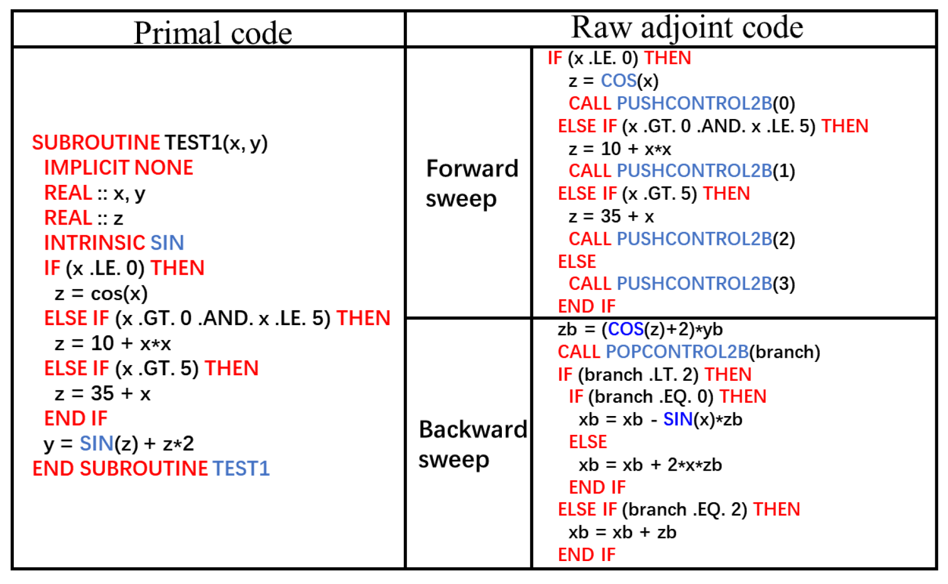
Figure 1. Case 1: the primal code and the raw adjoint code.
Aerospace 10 00106 g001
Figure 2. Case 2: the primal code and the raw adjoint code.
Aerospace 10 00106 g002
Figure 3. Case 1: the raw adjoint code and the hybrid adjoint code.
Aerospace 10 00106 g003
Figure 4. Case 2: the raw adjoint code and the hybrid adjoint code.
Aerospace 10 00106 g004
Figure 5. The flow codes corresponding to the calculation of convective flux.
Aerospace 10 00106 g005
Figure 6. The raw adjoint codes corresponding to the calculation of convective flux.
Aerospace 10 00106 g006
Figure 7. The hybrid adjoint codes corresponding to the calculation of convective flux.
Aerospace 10 00106 g007
Figure 9. Computational mesh used for the NASA Stage 35.
Aerospace 10 00106 g009
Figure 10. Isentropic efficiency against the mass flow rate at 100% design speed (a); Fine-grid solution, with discretization errors computed using the corresponding equations in reference [32] (b).
Aerospace 10 00106 g010
Figure 11. Total pressure ratio against the mass flow rate at 100% design speed (a); fine-grid solution, with discretization errors computed using the corresponding equations in reference [32] (b).
Aerospace 10 00106 g011
Figure 12. Flow and adjoint fields at 50% span of the NASA Stage 35. (a) Turbulence quantity. (b) Adjoint quantity corresponding to the turbulence model equation.
Aerospace 10 00106 g012
Figure 13. Comparison of sensitivity convergence histories among LIN, CEV, and hybrid ADJ for the NASA Stage 35.
Aerospace 10 00106 g013
Figure 14. Verification of sensitivity accuracy for the NASA Stage 35.
Aerospace 10 00106 g014
Figure 15. RMS residual convergence histories of both the flow and adjoint solvers (a); Comparison of CPU time among different solvers for the NASA Stage 35 (b).
Aerospace 10 00106 g015
Figure 16. Evolution histories of the weighted objective functions and constraints for the NASA Stage 35.
Aerospace 10 00106 g016
Figure 17. Comparison of performance characteristics at 100% design speed for the NASA Stage 35.
Aerospace 10 00106 g017
Figure 18. Comparison of blade profiles at three different spans for the NASA Stage 35.
Aerospace 10 00106 g018
Figure 19. Mach number contours at the middle span for the NASA Stage 35.
Aerospace 10 00106 g019
Figure 20. Radial distributions of rotor aerodynamic parameters at the peak efficiency point for the NASA Stage 35.
Aerospace 10 00106 g020
Figure 21. Radial distributions of stator aerodynamic parameters calculated across the stator only at the peak efficiency point for the NASA Stage 35.
Aerospace 10 00106 g021
Figure 22. Computational mesh used for the Aachen turbine.
Aerospace 10 00106 g022
Figure 23. Flow and adjoint fields at 50% span of the Aachen turbine. (a) Turbulence quantity. (b) Adjoint quantity corresponding to the turbulence model equation.
Aerospace 10 00106 g023
Figure 24. Comparison of sensitivity convergence histories for the Aachen turbine.
Aerospace 10 00106 g024
Figure 25. Verification of sensitivity accuracy for the Aachen turbine case.
Aerospace 10 00106 g025
Figure 26. RMS residual convergence histories of both the flow and adjoint solvers (a); comparison of CPU time among different solvers for the Aachen turbine (b).
Aerospace 10 00106 g026
Figure 27. Evolution histories of the weighted objective function and constraints for the Aachen turbine.
Aerospace 10 00106 g027
Figure 28. Comparison of original and optimized blade profiles at three different spans for the Aachen turbine.
Aerospace 10 00106 g028
Figure 29. Radial distributions of total pressure ratio, inlet, and outlet flow angles in each row for the Aachen turbine.
Aerospace 10 00106 g029aAerospace 10 00106 g029b
Table 1. Grid nodes in the three coordinate directions for NASA stage 35.
      AxialCircumferentialRadialTotal
Row 1Grid11333757∼280 k
   Grid21495773∼620 k
   Grid31618589∼1218 k
Row 2Grid11453357∼273 k
   Grid21614961∼481 k
   Grid31696181∼835 k
Table 2. Comparison of time and memory consumption among different solvers for the NASA Stage 35.
   FlowOriginal ADJHybrid ADJ
time16.163.49 (−43%)
memory12.522.29 (−9%)
Table 3. Comparison of aerodynamic performances between the original and optimized blade profiles for the NASA Stage 35.
      m(kg/s) π η ( % )
chokeoriginal21.021.74583.35
   optimized21.05 (+0.14%)1.745 (0%)84.00 (+0.65)
peakoriginal20.971.83583.91
   optimized21.00 (+0.14%)1.835 (0%)84.73 (+0.82)
stalloriginal20.601.92482.19
   optimized20.55 (−0.24%)1.922 (−0.10%)82.67 (+0.48)
Table 4. Comparison of time and memory consumption among different solvers for the Aachen turbine.
   FlowOriginal ADJHybrid ADJ
time16.163.43 (−44%)
memory11.941.77 (−9.6%)
Disclaimer/Publisher’s Note: The statements, opinions and data contained in all publications are solely those of the individual author(s) and contributor(s) and not of MDPI and/or the editor(s). MDPI and/or the editor(s) disclaim responsibility for any injury to people or property resulting from any ideas, methods, instructions or products referred to in the content.