
Supercritical Injection Modeling by an Incompressible but Variable Density Approach


Abstract
:1. Introduction
2. Governing Equations
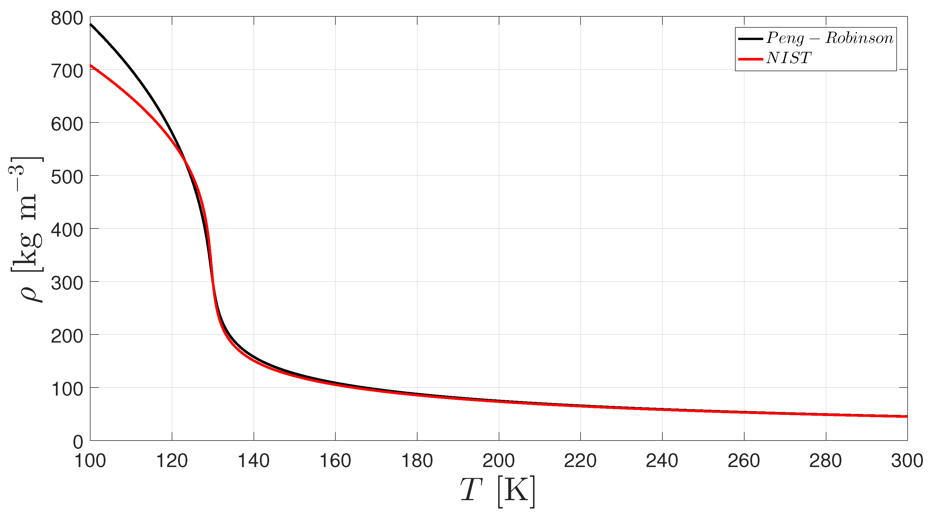
3. Equation of State
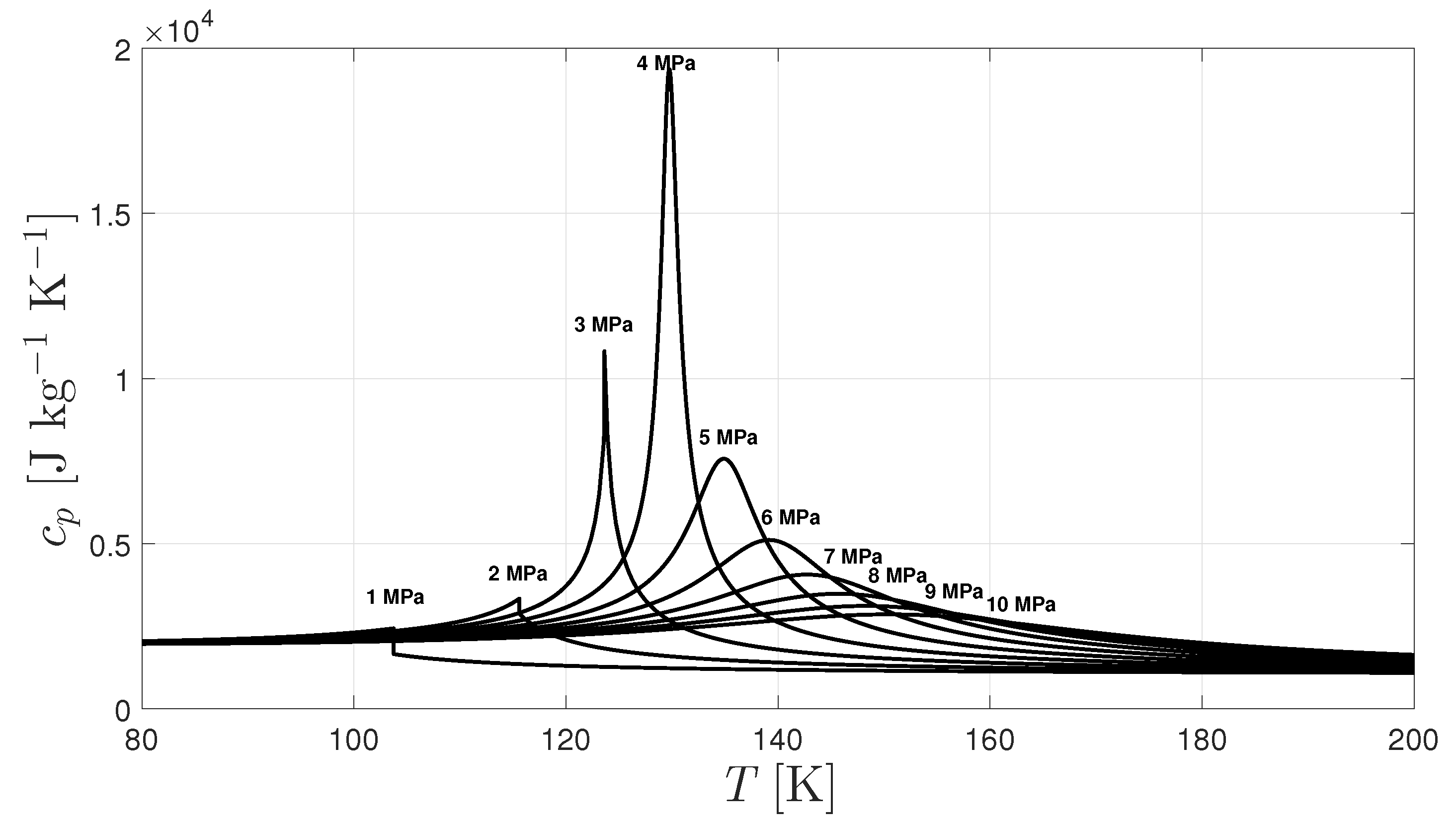
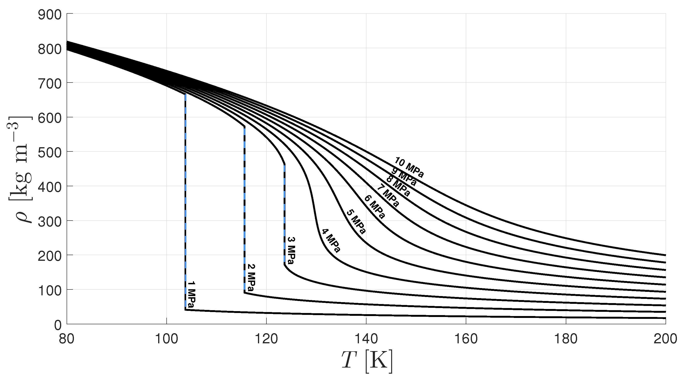
4. Thermodynamic Properties
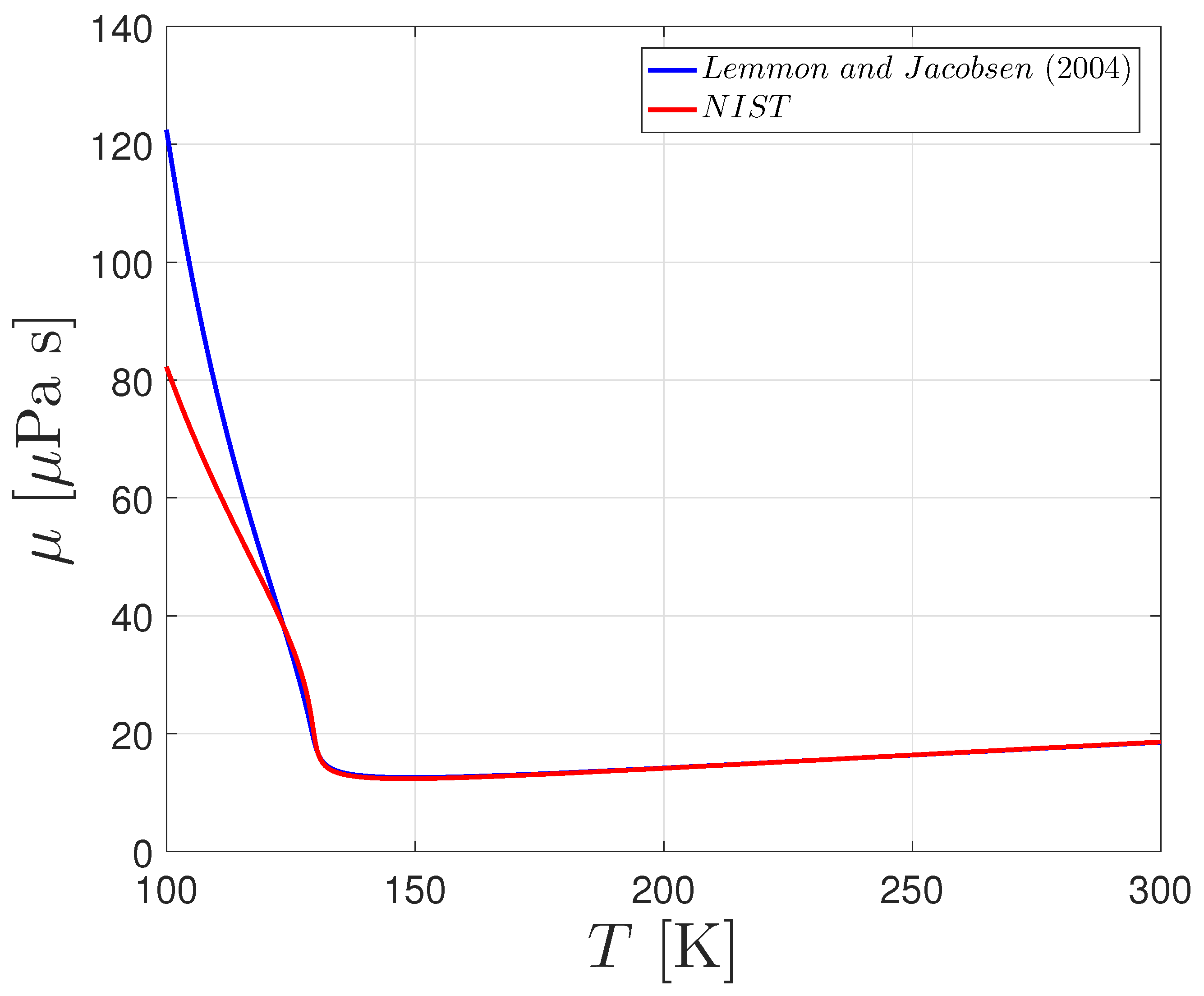
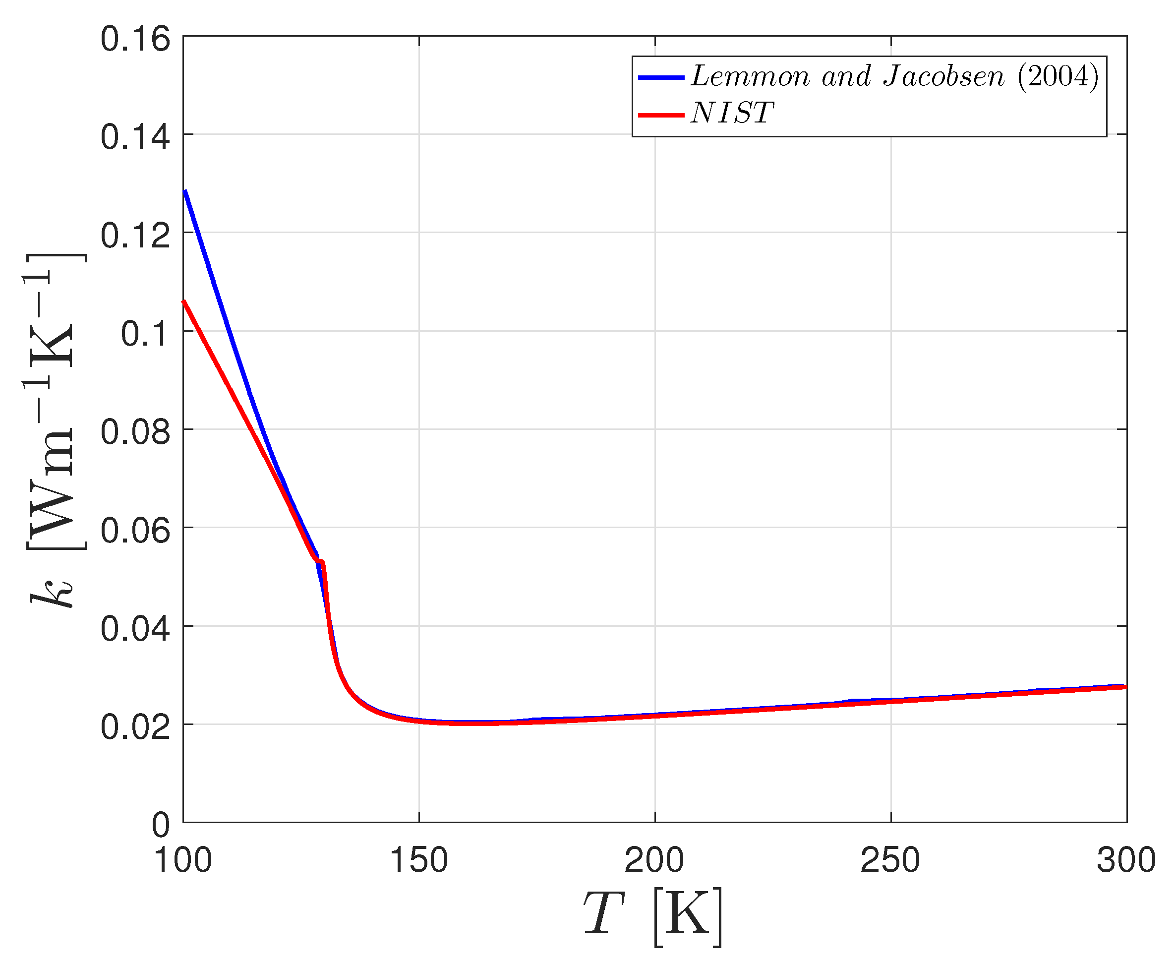
5. Transport Properties
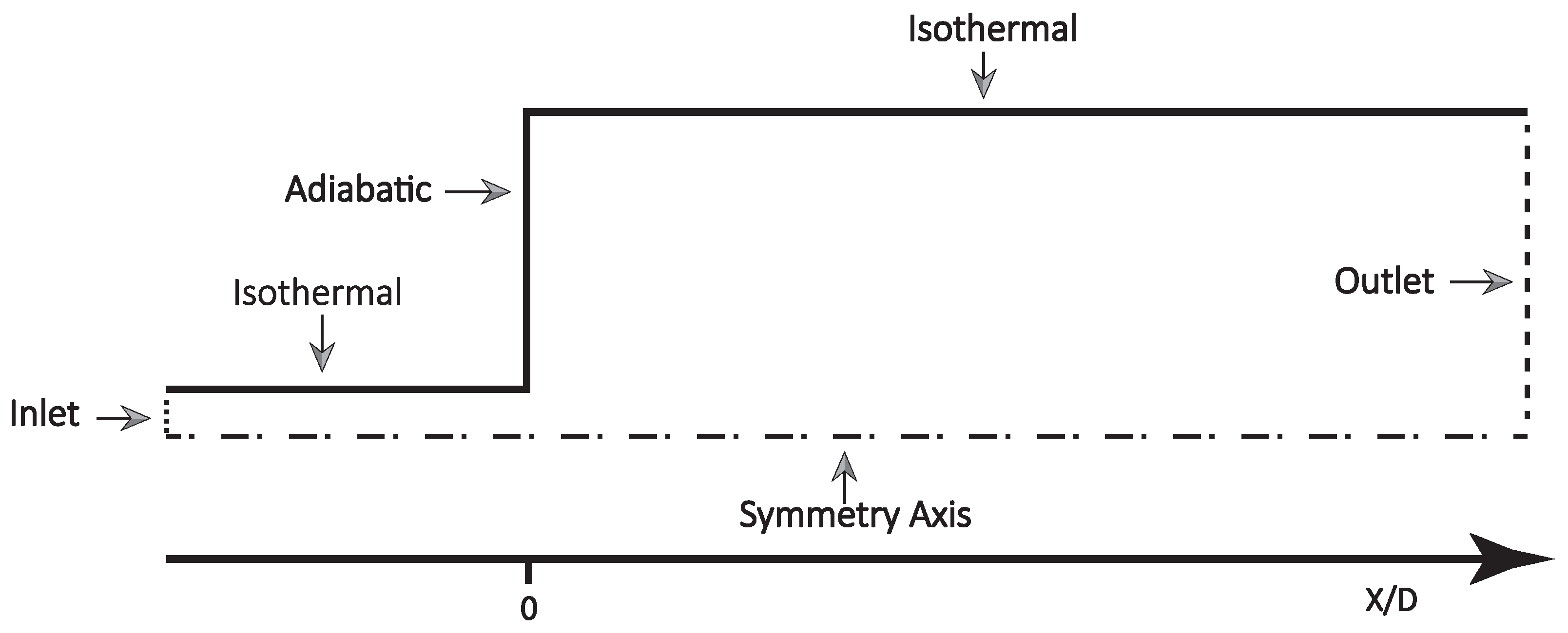
6. Computational Methods
7. Experimental Conditions Analysis
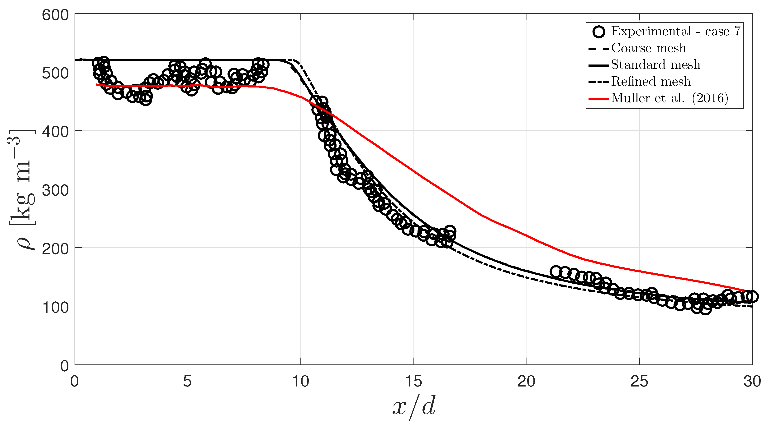
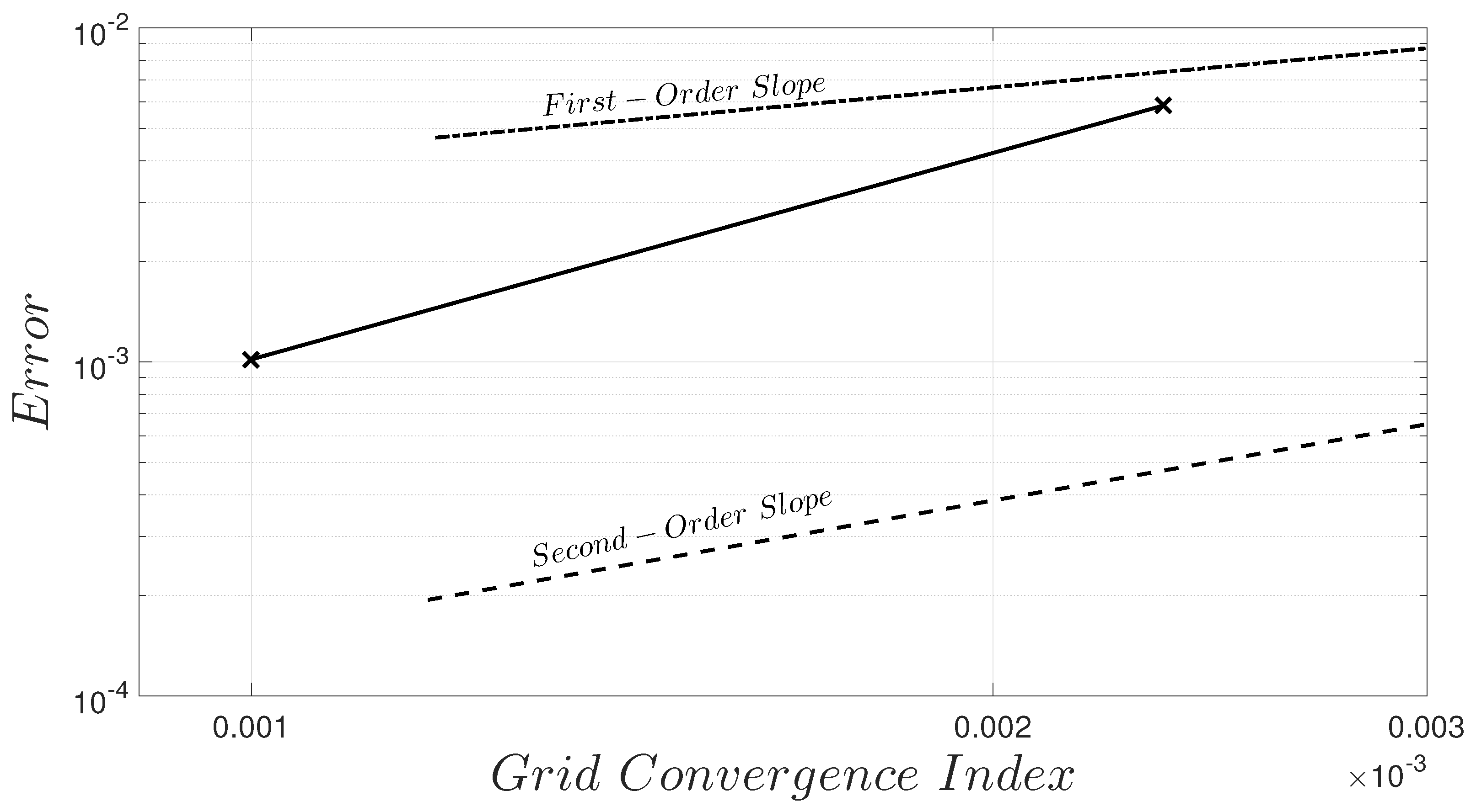
8. Results
9. Conclusions
Author Contributions
Funding
Data Availability Statement
Conflicts of Interest
Abbreviations
| BC | Boundary Condition |
| DNS | Direct Numerical Simulation |
| GCI | Grid Convergence Index |
| LES | Large Eddy Simulation |
| LRE | Liquid Rocket Engine |
| NASA | National Aeronautics and Space Administration |
| NIST | National Institute of Standards |
| RANS | Reynolds-averaged Navier–Stokes |
| QUICK | Quadratic Upstream Interpolation for Convective Kinematics |
References
- Gao, Z.; Bai, J.; Zhou, J.; Wang, C.; Li, P. Numerical Investigation of Supercritical Methane in Helically Coiled Tube on Regenerative Cooling of Liquid Rocket Electromechanical Actuator. Cryogenics 2020, 106, 103023. [Google Scholar] [CrossRef]
- Segal, C.; Polikhov, S.A. Subcritical to Supercritical Mixing. Phys. Fluids 2008, 20, 052101. [Google Scholar] [CrossRef]
- DeSouza, S.; Segal, C. Sub- and Supercritical Jet Disintegration. Phys. Fluids 2017, 29, 47–107. [Google Scholar] [CrossRef]
- Jofre, L.; Urzay, J. Transcritical Diffuse-interface Hydrodynamics of Propellants in High-pressure Combustors of Chemical Propulsion Systems. Prog. Energy Combust. Sci. 2021, 82, 100877. [Google Scholar] [CrossRef]
- Davis, D.W.; Chehroudi, B. Measurements in an Acoustically Driven Coaxial Jet under Sub-, Near-, and Supercritical Conditions. J. Propuls. Power 2007, 23, 364–374. [Google Scholar] [CrossRef]
- Roy, A.; Segal, C. Experimental Study of Fluid Jet Mixing at Supercritical Conditions. J. Propuls. Power 2010, 26, 1205–1211. [Google Scholar] [CrossRef]
- Banuti, D.T. Crossing the Widom-line–Supercritical Pseudo-boiling. J. Supercrit. Fluids 2015, 98, 12–16. [Google Scholar] [CrossRef]
- Raju, M.; Banuti, D.T.; Ma, P.C.; Ihme, M. Widom Lines in Binary Mixtures of Supercritical Fluids. Sci. Rep. 2017, 3027. [Google Scholar] [CrossRef] [Green Version]
- Linstrom, P.J.; Mallard, W.G. (Eds.) NIST Chemistry WebBook, NIST Standard Reference Database 69; National Institute of Standards and Technology: Gaithersburg, MD, USA, 1997. [Google Scholar] [CrossRef]
- Maxim, F.; Contescu, C.; Boillat, P.; Niceno, B.; Karalis, K.; Testino, A.; Ludwig, C. Visualization of Supercritical Water Pseudo-boiling at Widom Line Crossover. Nat. Commun. 2019, 10, 4114. [Google Scholar] [CrossRef] [PubMed] [Green Version]
- Banuti, D.T. A Thermodynamic Look at Injection in Aerospace Propulsion Systems. In Proceedings of the AIAA Scitech 2020 Forum, Orlando, FL, USA, 6–10 January 2020. [Google Scholar] [CrossRef]
- Banuti, D.T.; Raju, M.; Ma, C.; Ihme, M.; Hickey, J. Seven Questions about Supercritical Fluids—Towards a New Fluid State Diagram. In Proceedings of the 55th AIAA Aerospace Sciences Meeting, Grapevine, TX, USA, 9–13 January 2017. [Google Scholar] [CrossRef] [Green Version]
- Poormahmood, A.; Farshchi, M. Numerical Study of the Mixing Dynamics of Trans- and Supercritical Coaxial Jets. Phys. Fluids 2020, 32, 125105. [Google Scholar] [CrossRef]
- Lapenna, P.E. Characterization of Pseudo-boiling in a Transcritical Nitrogen Jet. Phys. Fluids 2018, 30, 77–106. [Google Scholar] [CrossRef]
- Zong, N.; Meng, H.; Hsieh, S.; Yang, V. A Numerical Study of Cryogenic Fluid Injection and Mixing under Supercritical Conditions. Phys. Fluids 2004, 16, 4248–4261. [Google Scholar] [CrossRef] [Green Version]
- Schmitt, T.; Rodriguez, J.; Leyva, I.A.; Candel, S. Experiments and Numerical Simulation of Mixing under Supercritical Conditions. Phys. Fluids 2012, 24, 55–104. [Google Scholar] [CrossRef]
- Terashima, H.; Koshi, M. Strategy for Simulating Supercritical Cryogenic Jets using High-order Schemes. Comput. Fluids 2013, 85, 39–46. [Google Scholar] [CrossRef]
- Banuti, D.T.; Hannemann, K. The Absence of a Dense Potential Core in Supercritical Injection: A Thermal Break-up Mechanism. Phys. Fluids 2016, 28, 035103. [Google Scholar] [CrossRef]
- Traxinger, C.; Zips, J.; Pfitzner, M. Single-phase Instability in Non-premixed Flames under Liquid Rocket Engine Relevant Conditions. J. Propuls. Power 2019, 35, 1–15. [Google Scholar] [CrossRef]
- Lacaze, G.; Schmitt, T.; Ruiz, A.; Oefelein, J.C. Comparison of Energy-, Pressure- and Enthalpy-based Approaches for Modeling Supercritical Flows. Comput. Fluids 2019, 181, 35–56. [Google Scholar] [CrossRef] [Green Version]
- Kim, N.; Kim, Y. Large Eddy Simulation Based Multi-environment PDF Modelling for Mixing Processes of Transcritical and Supercritical Cryogenic Nitrogen Jets. Cryogenics 2020, 110, 103134. [Google Scholar] [CrossRef]
- Ruan, B.; Lin, W. Numerical Investigation on Heat Transfer and Flow Characteristics of Supercritical Methane in a Horizontal Tube. Cryogenics 2022, 124, 103482. [Google Scholar] [CrossRef]
- Mayer, W.; Telaar, J.; Branam, R.; Schneider, G.; Hussong, J. Raman Measurements of Cryogenic Injection at Supercritical Pressure. Heat Mass Transf. 2003, 39, 709–719. [Google Scholar] [CrossRef]
- Cheng, G.C.; Farmer, R. Real Fluid Modeling of Multiphase Flows in Liquid Rocket Engine Combustors. J. Propuls. Power 2006, 22, 1373–1381. [Google Scholar] [CrossRef]
- Schmitt, T.; Selle, L.; Ruiz, A.; Cuenot, B. Large-Eddy Simulation of Supercritical-Pressure Round Jets. AIAA J. 2010, 48, 2133–2144. [Google Scholar] [CrossRef]
- Jarczyk, M.; Pfitzner, M. Large Eddy Simulation of Supercritical Nitrogen Jets. In Proceedings of the 50th AIAA Aerospace Sciences Meeting, Nashville, TN, USA, 9–12 January 2012. [Google Scholar] [CrossRef] [Green Version]
- Ma, P.C.; Lv, Y.; Ihme, M. An Entropy-stable Hybrid Scheme for Simulations of Transcritical Real-fluid Flows. J. Comput. Phys. 2017, 340, 330–357. [Google Scholar] [CrossRef]
- Ries, F.; Obando, P.; Shevchuck, I.; Janicka, J.; Sadiki, A. Numerical Analysis of Turbulent Flow Dynamics and Heat Transport in a Round Jet at Supercritical Conditions. Int. J. Heat Fluid Flow 2017, 66, 172–184. [Google Scholar] [CrossRef]
- Ries, F.; Janicka, J.; Sadiki, A. Thermal Transport and Entropy Production Mechanisms in a Turbulent Round Jet at Supercritical Thermodynamic Conditions. Entropy 2017, 19, 404. [Google Scholar] [CrossRef] [Green Version]
- Taghizadeh, S.; Jarrahbashi, D. Proper Orthogonal Decomposition Analysis of Turbulent Cryogenic Liquid Jet Injection Under Transcritical and Supercritical Conditions. At. Sprays 2018, 28, 875–900. [Google Scholar] [CrossRef]
- Li, L.; Xie, M.; Wei, W.; Jia, M.; Liu, H. Numerical Investigation on Cryogenic Liquid Jet under Transcritical and Supercritical Conditions. Cryogenics 2018, 89, 16–28. [Google Scholar] [CrossRef]
- Lagarza-Cortés, C.; Ramírez-Cruz, J.; Salinas-Vázquez, M.; Rodríguez, W.V.; Cubos-Ramírez, J.M. Large-eddy Simulation of Transcritical and Supercritical Jets Immersed in a Quiescent Environment. Phys. Fluids 2019, 31, 025104. [Google Scholar] [CrossRef]
- Ningegowda, B.M.; Rahantamialisoa, F.; Zembi, J.; Pandal, A.; Im, H.G.; Battistoni, M. Large Eddy Simulations of Supercritical and Transcritical Jet Flows Using Real Fluid Thermophysical Properties; SAE Technical Paper Series; SAE International: Warren Dale, PA, USA, 2020. [Google Scholar] [CrossRef]
- Ries, F.; Kütemeier, D.; Li, Y.; Nishad, K.; Sadiki, A. Effect Chain Analysis of Supercritical Fuel Disintegration Processes Using an LES-based Entropy Generation Analysis. Combust. Sci. Technol. 2020, 1–18. [Google Scholar] [CrossRef]
- Ma, J.; Liu, H.; Liu, L.; Xie, M. Simulation Study on the Cryogenic Liquid Nitrogen Jets: Effects of Equations of State and Turbulence Models. Cryogenics 2021, 117, 103330. [Google Scholar] [CrossRef]
- Magalhães, L.B.; Silva, A.R.R.; Barata, J.M.M. Contribution to the Physical Description of Supercritical Cold Flow Injection: The Case of Nitrogen. Acta Astronaut. 2022, 190, 251–260. [Google Scholar] [CrossRef]
- Bellan, J. Future Challenges in the Modelling and Simulations of High-pressure Flows. Combust. Sci. Technol. 2020, 192, 1199–1218. [Google Scholar] [CrossRef]
- Newman, J.A.; Brzustowksi, T.A. Behavior of a Liquid Planar Jet Near the Thermodynamic Critical Region. AIAA J. 1971, 9, 1595–1602. [Google Scholar] [CrossRef]
- Chehroudi, B.; Talley, D.; Coy, E. Visual Characteristics and Initial Growth Rates of Round Cryogenic Jets at Subcritical and Supercritical Pressures. Phys. Fluids 2002, 14, 850–861. [Google Scholar] [CrossRef]
- Oschwald, M.; Schik, A.; Klar, M.; Mayer, W. Investigation Of Coaxial LN2/GH2-injection at Supercritical Pressure by Spontaneous Raman Scattering. In Proceedings of the 35th Joint Propulsion Conference and Exhibit, Los Angeles, CA, USA, 20–24 June 1999. [Google Scholar] [CrossRef]
- Oschwald, M.; Smith, J.J.; Braman, R.; Hussong, J.; Schik, A.; Chehroudi, B.; Talley, D.G. Injection of Fluids into Supercritical Environments. Combust. Sci. Technol. 2006, 178, 49–100. [Google Scholar] [CrossRef]
- Banuti, D. Thermodynamic Analysis and Numerical Modeling of Supercritical Injection. Ph.D. Thesis, Institute of Aerospace Thermodynamics, University of Stuttgart, Stuttgart, Germany, 2015. [Google Scholar]
- Lapenna, P.E.; Creta, F. Mixing under Transcritical Conditions: An A-priori Study Using Direct Numerical Simulation. J. Supercrit. Fluids 2017, 128, 263–278. [Google Scholar] [CrossRef]
- Barata, J.; Gökalp, I.; Silva, A. Numerical Study of Cryogenic Jets under Supercritical Conditions. J. Propuls. Power 2003, 19, 142–147. [Google Scholar] [CrossRef]
- Launder, B.E.; Spalding, D.B. Lectures in Mathematical Models of Turbulence; Academic Press: London, UK, 1972. [Google Scholar]
- Park, T.S. LES and RANS Simulations of Cryogenic Liquid Nitrogen Jets. J. Supercrit. Fluids 2012, 72, 232–247. [Google Scholar] [CrossRef]
- Magalhães, L.; Carvalho, F.; Silva, A.; Barata, J. Turbulence Modeling Insights into Supercritical Nitrogen Mixing Layers. Energies 2020, 13, 1586. [Google Scholar] [CrossRef] [Green Version]
- Park, T.S. Application of κ-ϵ Turbulence Models with Density Corrections to Variable Density Jets under Subcritical/supercritical Conditions. Numer. Heat Transf. Part A Appl. 2019, 77, 162–178. [Google Scholar] [CrossRef]
- Kawai, S.; Oikawa, Y. Turbulence Modeling for Turbulent Boundary Layers at Supercritical Pressure: A Model for Turbulent Mass Flux. Flow Turbul. Combust. 2019, 104, 625–641. [Google Scholar] [CrossRef]
- Xiao, H.; Cinnella, P. Quantification of Model Uncertainty in RANS Simulations: A Review. Prog. Aerosp. Sci. 2019, 108, 1–31. [Google Scholar] [CrossRef] [Green Version]
- Otero, G.J.; Patel, A.; Diez, R.; Pecnik, R. Turbulence modelling for flows with strong variations in thermo-physical properties. Int. J. Heat Fluid Flow 2018, 73, 114–123. [Google Scholar] [CrossRef]
- Cook, L.W.; Mishra, A.A.; Jarrett, J.P.; Willcox, K.E.; Iaccarino, G. Optimization Under Turbulence Model Uncertainty for Aerospace Design. Phys. Fluids 2019, 31, 105111. [Google Scholar] [CrossRef]
- Ghanbari, M.; Ahmadi, M.; Lashanizadegan, A. A Comparison between Peng-Robinson and Soave-Redlich-Kwong Cubic Equations of State from Modification Perspective. Cryogenics 2017, 84, 13–19. [Google Scholar] [CrossRef]
- Peng, D.; Robinson, D.B. A New Two-constant Equation of State. Ind. Eng. Chem. Fundam. 1976, 15, 59–64. [Google Scholar] [CrossRef]
- McBride, B.J.; Zehe, M.J.; Gordon, S. NASA Glenn Coefficients for Calculating Thermodynamic Properties of Individual Species; Technical Report; NASA/TP–2002-211556; NASA Glenn Research Center: Cleveland, OH, USA, 2002. [Google Scholar]
- Reid, R.C.; Prausnitz, J.M.; Poling, B.E. The Properties of Gases and Liquids; McGraw-Hill, Inc.: New York, NY, USA, 1987. [Google Scholar]
- Lemmon, E.W.; Jacobsen, R.T. Viscosity and Thermal Conductivity Equations for Nitrogen, Oxygen, Argon and Air. Int. J. Thermophys. 2004, 25, 21–69. [Google Scholar] [CrossRef]
- Olchowy, G.A.; Sengers, J.V. A Simplified Representation for the Thermal Conductivity of Fluids in the Critical Region. Int. J. Thermophys. 1989, 10, 417–426. [Google Scholar] [CrossRef]
- Span, R.; Lemmon, E.W.; Jacobsen, R.T.; Wagner, W. A Reference Quality Equation of State for Nitrogen. Int. J. Thermophys. 1998, 19, 1121–1132. [Google Scholar] [CrossRef]
- Leonard, B.P. A Stable and Accurate Convective Modelling Procedure Based on Quadratic Upstream Interpolation. Comput. Methods Appl. Mech. Eng. 1979, 19, 58–98. [Google Scholar] [CrossRef]
- Müller, H.; Niedermeier, C.A.; Jarczyk, M.; Pfitzner, M.; Hickel, S.; Adams, N.A. Large Eddy Simulation of Trans- and Supercritical Injection. Prog. Propuls. Phys. 2016, 8, 5–24. [Google Scholar] [CrossRef] [Green Version]
- Roache, P.J. Verification and Validation in Computational Science and Engineering; John Whiley & Sons: Albuquerque, NM, USA, 1998. [Google Scholar]
- Gopal, J.M.; Tretola, G.R.; Morgan, R.; de Sercey, G.; Atkins, A.; Vogiatzaki, K. Understanding Sub and Supercritical Cryogenic Fluid Dynamics in Conditions Relevant to Novel Ultra Low Emission Engines. Energies 2020, 13, 3038. [Google Scholar] [CrossRef]


| Coefficient | Value |
|---|---|
| 0.24159429 × 101 | |
| 0.17489065 × 10⁻³ | |
| −0.11902369 × 10⁶ | |
| 0.30226245 × 10⁻¹⁰ | |
| −0.20360982 × 10⁻¹⁴ | |
| 0.56133773 × 10⁵ |
| i | |
|---|---|
| 0 | 0.431 |
| 1 | −0.4623 |
| 2 | 0.08406 |
| 3 | 0.005341 |
| 4 | −0.00331 |
| i | ||||
|---|---|---|---|---|
| 1 | 10.72 | 0.1 | 2 | 0 |
| 2 | 0.03989 | 0.25 | 10 | 1 |
| 3 | 0.001208 | 3.2 | 12 | 1 |
| 4 | −7.402 | 0.9 | 2 | 2 |
| 5 | 4.620 | 0.3 | 1 | 3 |
| i | ||||
|---|---|---|---|---|
| 1 | 1.511 | - | - | - |
| 2 | 2.117 | −1.0 | - | - |
| 3 | −3.332 | −0.7 | - | - |
| 4 | 8.862 | 0.0 | 1 | 0 |
| 5 | 31.11 | 0.03 | 2 | 0 |
| 6 | −73.13 | 0.2 | 3 | 1 |
| 7 | 20.03 | 0.8 | 4 | 2 |
| 8 | −0.7096 | 0.6 | 8 | 2 |
| 9 | 0.2672 | 1.9 | 10 | 2 |
Disclaimer/Publisher’s Note: The statements, opinions and data contained in all publications are solely those of the individual author(s) and contributor(s) and not of MDPI and/or the editor(s). MDPI and/or the editor(s) disclaim responsibility for any injury to people or property resulting from any ideas, methods, instructions or products referred to in the content. |
© 2023 by the authors. Licensee MDPI, Basel, Switzerland. This article is an open access article distributed under the terms and conditions of the Creative Commons Attribution (CC BY) license (https://creativecommons.org/licenses/by/4.0/).
Share and Cite
Magalhães, L.B.; Silva, A.R.R.; Barata, J.M.M. Supercritical Injection Modeling by an Incompressible but Variable Density Approach. Aerospace 2023, 10, 114. https://doi.org/10.3390/aerospace10020114
Magalhães LB, Silva ARR, Barata JMM. Supercritical Injection Modeling by an Incompressible but Variable Density Approach. Aerospace. 2023; 10(2):114. https://doi.org/10.3390/aerospace10020114
Chicago/Turabian StyleMagalhães, Leandro B., André R. R. Silva, and Jorge M. M. Barata. 2023. "Supercritical Injection Modeling by an Incompressible but Variable Density Approach" Aerospace 10, no. 2: 114. https://doi.org/10.3390/aerospace10020114