A Fault Diagnosis Method under Data Imbalance Based on Generative Adversarial Network and Long Short-Term Memory Algorithms for Aircraft Hydraulic System

Abstract

Safe and stable operation of the aircraft hydraulic system is of great significance to the flight safety of an aircraft. Any fault may be a threat to flight safety and may lead to enormous economic losses and even human casualties. Hence, the normal status of the aircraft hydraulic system is large, but very few data samples relate to the fault status. This causes a data imbalance in the fault diagnosis of the aircraft hydraulic system, which directly affects the accuracy of aircraft fault diagnosis. To solve the data imbalance problem in the fault diagnosis of the aircraft hydraulic system, this paper proposes an improved GAN-LSTM algorithm by using the improved GAN method, which can stably and accurately generate high-quality simulated fault samples using a small number of fault data. First, the model of the aircraft hydraulic system was built using AMESim software, and the imbalanced fault data and normal status data were acquired. Then, the imbalanced data were used to train the GAN model until the system reached a Nash equilibrium. By comparing the time domain and frequency signal, it was found that the quality of the generated sample was highly similar to the real sample. Moreover, LSTM (long short-term memory) and some other data-driven intelligent fault diagnosis methods were used as classifiers. The accuracy of these fault diagnosis methods increased steadily when the number of fault samples was gradually increased until it reached a balance with the normal sample. Meanwhile, three different sample generation methods were compared and analyzed to find the method with the best data generation ability. Finally, the anti-noise performance of the LSTM-GAN method was analyzed; this model has superior noise immunity.

1. Introduction

Safe and stable operation of the aircraft hydraulic system is of great significance to the flight safety of an aircraft. Any fault may be a threat to flight safety and may lead to enormous economic losses and even human casualties. According to statistics, the probability of hydraulic system fault is greater than that of other systems [1]. Therefore, many scholars and researchers have studied fault diagnoses of the aircraft hydraulic system to explore effective methods to improve the accuracy of fault diagnosis [2,3,4]. Cui et al. built a grey fuzzy relation matrix by using grey fuzzy weight, membership, and degree of greyness and obtained a grey fuzzy attribute value based on expert weight. They determined the optimal maintenance decision of the aircraft hydraulic system based on the grey fuzzy attribute value [5]. Lin et al. modeled the extension and retraction problem of aircraft landing gear, selected the system output parameters, extracted the fault characteristics, and evaluated the health of the system by using a conventional forward neural network algorithm [6]. Wang et al. modeled the aircraft hydraulic pipe; they analyzed the natural frequency of the degree of hydraulic leakage fault, selected the natural frequencies of the first five orders as the characteristic value of the fault diagnosis, and conducted fault diagnosis by using a probabilistic neural network (PNN) [7]. Ma et al. analyzed the reliability of the aircraft hydraulic system by using the GO method, compared the calculated result of the GO method involving a feedback loop with the calculated result of the fault tree analysis method, and verified the validity of the GO method for reliability analysis and test evaluation of the aircraft hydraulic system [8]. In addition, some other machine learning methodologies have been performed on real datasets in vessels and wind farms [9,10]. Some researchers have studied the detection and isolation of sensor and actuator faults in flight control systems other than the hydraulic system [11,12,13,14].

Although these methods in the above papers have achieved good results, it is worth pointing out that most of the methods are data-driven fault diagnosis methods, which suffer from data imbalance in the process of data acquisition. Moreover, concerning the actual working status of the aircraft hydraulic system, the fault data and normal data are seriously imbalanced, and the time in the normal flight status is much greater than that under the fault status. In other words, in most cases, researchers encounter a fault data imbalance, which decreases the accuracy of fault diagnosis. Some solutions have been proposed to address the data imbalance in fault diagnosis [15,16,17]. However, the existing methods rely heavily on oversampling. Although oversampling can solve this data imbalance, it is hard to archive in real systems and costs too much money.

A GAN is an effective deep learning model that has two deep learning neural networks. Through the adversarial training of two neural networks, use of GANs attempts to achieve the goal of generating high-quality samples. Currently, GANs are used mostly in the fields of image processing and sound processing. Some researches want to improve the effect of GANs. Mao proposed the smallest two multiplication GAN (LS-GAN, least square GAN). Their discriminator in the adversarial training of the neural network used the minimum daily loss function, which increased the convergence speed and increased the training speed [18]. In the process of generating data, there are some cases that need to be generated in specific directions. Only using random vectors as generated inputs reduces the effect of generating data and reduces the speed of data generation. To solve this problem condition, GANs were proposed [19]. The network adds a specific label to the generator and the discriminator, which can guide the generating specific data through the label. In addition, there are many improved generating neural networks, including Pix2pix [20], VAE-GAN [21], Star-GAN [22]. These studies are all towards the purpose of improving CGAN to achieve guidance to achieve specific generated data.

Compared to the active results in the fields of image and sound processing, the beginnings of GANs being used in fault detection were relatively late. Now, some research has applied GANs to solve the data imbalance of fault diagnosis [23,24,25]. Zhou et al. improved the generator and identification device for generating adversarial networks to use the global optimization solution to generate more discrimination fault samples. This improved the accuracy and the effectiveness of the method was verified in an experiment on rolling bearings [26]. DIXIT et al. used an auxiliary conditioning classifier GAN that combined model-unrelated element learning (MAML). MAML was used to initialize and update network parameters instead of conventional random gradient learning, and then it was used to generate and classify the fault data set of bearings and air compressors [27]. AF et al. used a GAN combined temporal convolutional network (TCNN). Compared with the machine learning method SVM and the feed-forward neural network (FFNN), it was found that the combination of GAN and TCNN was better than the two methods mentioned above [28]. Wang et al. proposed a method of combining GAN and superimposed de-no-encoded self-encoders (SDAE), using SDAE as a GAN discriminator to automatically extract effective fault features from the input sample and judge their authenticity and fault category [29]. There are some other researchers who have studied the application of GAN in the field of fault diagnosis [30,31,32].

In this paper, an improved GAN method is proposed called ACWGAN-gp to solve the data imbalance problem in hydraulic systems. Using real data, together with class labels, we guided the generator model to generate fake data samples. Then, the discriminator judged the real samples and generated samples as fake or real. After training, a balance was achieved between the discriminator and generator. At this time, the discriminator could not judge whether a sample was fake or real. The generated samples were similar to the real samples in the characteristics, distribution, and status. Subsequently, the fault data were incremented by the generated data, and a balance was achieved between the fault data and normal data through continuous expansion. This method solves the data imbalance in the fault diagnosis of aircraft hydraulic systems. In addition, a LSTM method with four other data-driven methods was used in fault classification. This method provides a way to solve the data imbalance problem in the fault diagnosis of aircraft hydraulic systems. Our simulation results show the effectiveness and superiority of the proposed method.

The remainder of this paper is as follows. Section 2 describes the development of the proposed algorithm and fault detection method. Section 3 explains the fault data generation process. Section 4 presents the validation of the generated data by applying them to the LSTM fault diagnosis method together with four other methods, then compares them with two different data-generated models, then analyzes the anti-noise ability of the model. Finally, Section 5 concludes the paper.

2. Model Design of Fault Diagnosis

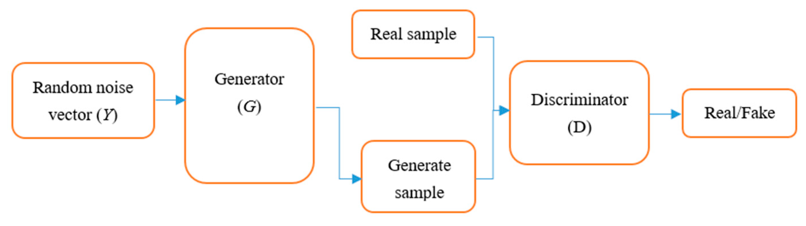
2.1. GAN Algorithm

The GAN (generative adversarial network) algorithm was proposed in 2014 to address the data imbalance in fault detection [33]. The GAN consists of a generator and discriminator. The generator is guided by a small number of actual data samples and generates data from random noise vectors to simulate the characteristics and status of the actual data. The discriminator is used for iteration to improve the quality of the generated data by discriminating the similarity between the generated data and actual data. The adversarial training of the two networks continues until the Nash equilibrium is achieved. The quality of the generated samples improves in the gaming of the generator and the discriminator. The generated data are closer to the actual data, and the discriminator cannot distinguish the data as actual data or generated data. Its loss function and objective function can be defined as:

$$L\left(G,D\right)=E_{s~p_{data}}\left[\log D\left(s\right)\right]+E_{y~P_y}\left[\log \left(1-D\left(G\left(y\right)\right)\right)\right]$$

(1)

$$Goal=\mathrm{argmin}\left(\mathrm{G}\right)\max \left(\mathrm{D}\right)\left[\mathrm{M}\left(\mathrm{G},\mathrm{D}\right)\right]$$

(2)

In Equations (1) and (2), G denotes the generator, D denotes the discriminator, P_data denotes the real data, P_y denotes a random noise vector, D(s) denotes the probability of s based on the real data, E_s∼Pdata denotes the expectation of s on the real data distribution P_data, and E_y∼Py denotes the expected value of y, which is sampled from the noise. The G objective function L (G, D) is minimized, whereas the D objective function L (G, D) is maximized. G and D converge when they reach the Nash equilibrium. The simple structure of GAN is in Figure 1.

The auxiliary classifier generative adversarial network (ACGAN) is an improvement of the GAN. The classifier items are introduced to the ACGAN to assist the generator in completing the data generation. The generator generates new samples, denoted as G (y, x), by using the random noise y and classifier label x∼p_x. The discriminator is required to recognize the generated samples and the correlated classifier items. Through adversarial training, the ACGAN is finally optimized in terms of data generation [34]. The real data and the classifier information should be processed; therefore, the objective of the ACGAN consists of the correct source L_source and correct class L_class. The loss function of this method can be expressed as:

$$L_{source}=E_{s~p_{data}}\left[\log D\left(s\right)\right]+E_{y~p_y}\left[\log \left(1-D\left(G\left(y\right)\right)\right)\right]$$

(3)

$$L_{class}=E_{s~p_{data}}\left[\log Q\left(X=x|Q_{real}\right)\right]+E_{y~p_y}\left[\log Q\left(X=x|Q_{generated}\right)\right]$$

(4)

The optimization objective of the discriminator is the maximization of L_source + L_class, whereas the training objective of the generator is the maximization of L_source − L_class. Despite being an excellent data generation model, GANs have certain limitations. The generator and discriminator in the training have problems such as vanishing gradient, non-convergence, and unstable training results, which reduce the effectiveness of the training.

To solve this problem, the WGAN was proposed by Arjovsky, which represents an important progress in the stable training of GANs [35,36]. Arjovsky attributed the instability of data training in the GAN model to an objective function in the form of J–S divergence and suggested evaluating the distance between the real samples and generated samples by using the Wasserstein distance rather than the J–S divergence. The objective function of the WGAN is:

$$Goa{l}_{wgan}=\underset{G}{\min }\underset{D\in \alpha }{\max }\left\{E_{s~p_{date}}\left[D\left(s\right)\right]-E_{y~p_y}D\left(G\left(y\right)\right)\right\}$$

(5)

where $\alpha$ denotes the set of the 1-Lipschitz function, which can be interpreted as a measurement function whose slope never exceeds one. Its weight lies within the compact space [−$\mathit{\omega }$, $\mathit{\omega }$]. Under the optimal discriminator, the value function of the minimized generator parameters is equivalent to the minimized Wasserstein distance. Compared with the GAN, the training process of the WGAN is more stable and faster.

Nevertheless, it sometimes fails to generate a high-quality sample or achieve convergence. Gulrajani attributed the problem to the use of weight clipping in the WGAN to execute Lipschitz’s constraint on the discriminator. Therefore, they proposed a method to improve the WGAN by introducing the concept of gradient penalty, namely, WGAN-gp [31]. Its loss function and objective function are as follows:

$$L_{w-gp}=E_{y~p_y}\left[D\left(G\left(y\right)\right)\right]-E_{s~p_{data}}\left[D\left(s\right)\right]+\mathsf{\lambda }{E}_{\widehat{s}~\widehat{p_s}}\left[{(\Vert {\nabla }_{\widehat{s}}D{\left(\widehat{s}\right)\Vert }_2-1)}^2\right]$$

(6)

$$Goa{l}_{w-gp}=\underset{G}{\min }\underset{D}{\max }\left\{E_{s~p_{date}}\left[D\left(s\right)\right]-E_{z~p_z}\left[D\left(G\left(z\right)\right)\right]-\mathsf{\lambda }{E}_{\widehat{s}~\widehat{p_s}}\left[{(\Vert {\nabla }_{\widehat{s}}D{\left(\widehat{s}\right)\Vert }_2-1)}^2\right]\right\}$$

(7)

where $\widehat{s}$ = $\mathit{\epsilon }$s + (1 − $\epsilon$) G (y), $\mathit{\epsilon }$ is a constant between zero and one, and $\mathsf{\lambda }$ represents a penalty coefficient. The detailed derivation process can be referred from the studies by Arjovsky et al. [35] and Gulrajani et al. [37].

2.2. Fault Detection Method Proposed in This Paper

To solve the data imbalance in the fault diagnosis, this paper proposes a method called ACWGAN-gp. The model can adaptively learn the original data distribution and then generate new samples to augment a small number of data classes. Then, the augmented dataset can be applied to a data-driven intelligent fault diagnosis method. The overall framework mainly includes three parts: sample pre-processing, sample generation and evaluation, and diagnosis of imbalanced faults. The flowchart is shown in Figure 2.

ACWGAN-gp is an improved GAN model to solve the data imbalance in the fault diagnosis of the aircraft hydraulic system. Specifically, ACWGAN-gp builds a new GAN model by introducing the Wasserstein distance and gradient penalty. The generator consists of a random noise vector Y and a sample vector X with a specific classifier. The new samples are generated through the generator. The new samples and real samples are imported into the discriminator for adversarial training. The discriminator is used to determine the true or false state of the sample and recognize its class. After satisfying the similarity criterion, the generated samples are applied to augment the original fault datasets to perform fault diagnosis analysis of the aircraft hydraulic system. The system architecture of the ACWGAN-gp algorithm is shown in Figure 3. S_R is a real sample set. S_G is a data sample set generated using the generator. S_G-R is a data sample set obtained using the discriminator with the same nature as the real dataset.

2.3. Design of Generator and Discriminator in the GAN Model

The generator and discriminator of the system were designed based on a two-dimensional convolutional neural network (2D-CNN). The input of the generator includes a noise vector Y and a classifier vector X. The input layer is linked to a fully connected layer having 1024 nodes. The output of the fully connected layer is transformed into an image (2 × 2 × 256, i.e., width: 2 units, height: 2 units; number of channels: 256) by the reshape function. The fully connected layer is followed by four consecutive two-dimensional deconvolution layers.

The first three deconvolution layers have 128, 64, and 32 filters, whereas the last deconvolution layer has only one filter. After the four deconvolution layers, the input data are transformed into a two-dimensional matrix. All pooling layers are removed. In the G network, the transposed convolutional layer is used for sampling. In the D network, convolution with stride is used instead of pooling. Before inputting to the discriminator, the two-dimensional matrix is reshaped into one-dimensional data and normalization is performed.

The structure of the discriminator is almost symmetric to that of the generator, and the input data are first reshaped into a two-dimensional matrix (32 × 32). Through the four convolutional layers, the data are transformed into 256 two-dimensional matrixes (2 × 2). After the last convolutional layer, the two-dimensional data are transformed back to one-dimensional data by the reshape function. Finally, the output layer is assigned a source classifier and class classifier. The structure diagrams of the generator and discriminator are shown in Figure 4.

Owing to the powerful sample generation performance of the GAN and powerful characteristic extraction capability, ACWGAN-GP can generate high-quality fault samples with the classifier by using the imbalanced dataset, which is of great significance in imbalanced fault diagnosis in actual hydraulic systems.

2.4. Model Description and Evaluation of ACWGAN-gp

Random noise vectors P_y, where Y = (y₁, y₂, y₃, …, y_m), and classifier set X = (x₁, x₂, x₃, …, x_k) are input to the generator for generating the synthesized sample S_G = G (y, x); the data distribution P_g of the synthesized samples is similar to that of the actual sample P_data. Next, the new sample S_G is mixed with the original sample S_R = (s₁, s₂, s₃, …, s_n) and provided as input to the discriminator for true and false discrimination. The generator and discriminator networks are trained alternately until a Nash equilibrium is reached. According to the Equations (3), (4), (6), and (7), the objective function of ACWGAN-GP can be obtained as follows:

$$L_D=E_{s~p_{data}}\left[\log D\left(s\right)\right]-E_{\tilde{s}~p_G}\left[\log D\left(\tilde{s}\right)\right]-\mathsf{\lambda }{E}_{\widehat{s}~p_{\widehat{s}}}\left[{(\Vert {\nabla }_{\widehat{s}}D{\left(\widehat{s}\right)\Vert }_2-1)}^2\right]+E_{s~p_{data}}\left[\log Q\left(\mathrm{X}=\left(x|Q_{real}\right)\right)\right]$$

(8)

$$L_G=E_{\tilde{s}~p_G}\left[\log D\left(\tilde{s}\right)\right]+E_{\tilde{s}~p_G}\left[\mathrm{logQ}\left(\mathrm{X}=\left(x|\tilde{s}\right)\right)\right]$$

(9)

In the above equations, $\tilde{\mathit{s}}$ is generated samples, $\hat{\mathit{s}}=\epsilon \mathit{s}+\left(1-\epsilon \right) \tilde{\mathit{s}}~{\mathit{p}}_{\widehat{\mathit{s}}}$ is the random sample obtained by interpolation on the s and $\tilde{s}$ lines; λ is a gradient penalty coefficient; and $Q\left(\mathrm{X}=\left(x|Q_{real}\right)\right)$ represents the conditional probability distribution on the classifier. To verify this method, the quality of the generated samples and their effect on the diagnosis of the imbalanced faults need to be evaluated. The validity of the generated data is examined by comparing the spectrum of the fault data generated through simulation with that of the original data.

3. Data Acquisition and Generation of the Aircraft Hydraulic System

3.1. Acquisition of Normal and Fault Data of Aircraft Hydraulic System

In this paper, the hydraulic system of a large passenger aircraft was adopted as the simulation object, and LMS AMESIM was employed to build the hydraulic system model, as shown in Figure 5. The hydraulic system of a passenger aircraft is composed of three relatively independent systems: main oil supply system 1, main oil supply system 2, and a back-up supply system. Main oil supply system 1 is powered by the left engine drive pump (EDP 2); main oil supply system 2 is powered by the right engine drive pump (EDP 12) under normal conditions. When both systems are broken down, the hydraulic system is driven by the ram air turbine (RAT 14) in the case of emergencies. The three electric driver pumps (EMP3, EMP13, EMP15) in the oil supply system are auxiliary energy; they help the two EDPs finish the hydraulic targets.

The main parameters used in the simulation are listed in

Table 1. Parameters of the simulation system.

No.	Element Names	Meaning	Parameter Value
1	Booster tank	Provides hydraulic oil	Preset pressure: 50 psi
2	Engine-driven pump 1	Provides power for aircraft hydraulics	Rpm: 5000 rec/min
3	Electrical-motor-driven pump 1	Auxiliary EDP1 oil supply	Rpm: 5000 rec/min
4	Throttle valve	Controls hydraulic flow	/
5	One-way valve	Prevents hydraulic oil backflow	/
6	Hydraulic oil filter	Prevents impurities in hydraulic filtration	/
7	Relief pressure control valve	Reduces the pressure, prevents too high pressure	Open: 3400 psi Close: 3200 psi
8	Hydraulic accumulator	Reduces the pulse of pressure and assists energy supply	Preset pressure: 1800 psi
9	Two-position three-way directional control valve	Control PTU	/
10	Three-position four-way directional control valve	Control actuator	/
11	Actuator	The mechanical part of the aircraft hydraulic system	/
12	EMP2	Auxiliary EDP2 oil supply	Rpm: 5000 rec/min
13	EDP2	Provides power for aircraft hydraulics	Rpm: 5000 rec/min
14	RAT	Provides an emergency power source for the aircraft hydraulic system	Rpm: 4000 rev/min
15	EMP3	Auxiliary oil supply	Rpm: 5000 rec/min
16	Hydraulic oil	Used to set the types and parameters of hydraulic oil	Density: 1003 g/L

. The numbers in this table are the hydraulic components in Figure 5. The normal simulation model was built considering stable conditions for the system. Under these normal operating conditions for the system, supply system 1 (Figure 5) and actuator 11 (Figure 5) were employed for the normal-mode hydraulic system in the simulations and analyses.

Three common faults, namely pump leak, actuator leak, and hydraulic oil pollution, were selected for the fault insertion, and the fault status was set as normal, moderate, or severe. The fault classification and fault parameter settings are shown in

Table 2. Parameters of the fault mode insertion.

Component Number	Type of Inserted Fault	Fault Mode Parameters	Normal Status	Moderate Fault	Severe Fault
2	Pump leak	Equivalent aperture/mm	0.1–0.5	0.5–1.0	1.5–2
11	Actuator leakage	Leak coefficient	0–0.01	0.05–0.09	0.1–0.15
16	Hydraulic oil pollution	Gas content/%	0.1–0.3	5–10	15–20

. The specific parameter settings of the components in this table were referred from previous studies [38,39].

The three types of fault data, namely actuator leak, hydraulic oil pollution, and pump leak, were selectively acquired. The status was set as normal, moderate fault, or severe fault. The acquired data simulated the extension and retraction process of the landing gear. The total duration was set to 20 s, in which the actuator did not operate from 0 to 2 s, performed the retraction movement of the landing gear from 2 to 7 s, stopped its operation from 7 to 9 s, performed the extension movement of the landing gear from 9 to 14 s, and shut down from 14 to 20 s. The sampling frequency was 100 Hz, and each simulation generated a dataset with length of 2000. The pressure sensor was placed at the position of the pump outlet. Figure 6 shows the time domain diagrams for comparing the acquired normal status signal with the other six types of fault status signals.

3.2. Generation of the Aircraft Hydraulic System Fault Sample

Seven types of data were acquired through the AMESim hydraulic system. One normal statue sample and six fault status samples were acquired. Firstly, 1200 normal samples were acquired through the simulation. Of these, 1000 samples were randomly selected as the training data, and 200 samples were randomly selected as the test data. After that, six types of faults were simulated. The fault statue dataset was generated by changing the range of the corresponding parameters in the simulation. Then, 300 fault samples were acquired through the simulation, of which 100 fault data were randomly selected as the training data, and 200 samples were randomly selected as the test data. Two hundred samples were selected from the fault/normal status data samples as the test data. In the training set, the normal status signal was regarded as the majority class set, and other fault classes were regarded as the minority class set, causing a fault imbalance problem. The attributes of the specifically acquired datasets are shown in

Table 3. Specific parameters and classifications of the generated fault datasets.

Classification of Sample Sets	Sample Length	Training Set	Test Set	Class Classifier
Normal status	2000	1000	200	0
Actuator leak (mild)	2000	100	200	1
Actuator leak (severe)	2000	100	200	2
Hydraulic oil pollution (mild)	2000	100	200	3
Hydraulic oil pollution (severe)	2000	100	200	4
Pump leak (mild)	2000	100	200	5
Pump leak (severe)	2000	100	200	6

.

The GAN model was trained to generate the six classifiers of the fault samples for the aircraft hydraulic system data. The GAN network model was established according to the method in Section 2 by using MATLAB, and the model was trained to finally achieve the adversarial balance between the generator and discriminator. It could generate samples with attributes similar to those of the real samples. In the sample generation process, the recorded values of the loss function were used to characterize the performance of the model. The training loss functions of the generator and discriminator are shown in Figure 7.

According to Figure 7, the loss curves of the generator and discriminator decrease significantly at the beginning and then gradually increase as the number of iterations increases. After approximately 1500 iterations, the generator loss converges to a constant value less than one. After approximately 1000 iterations, the discriminator loss converges to a constant near zero. After 4000 trainings, the discriminator discriminates the real probability of the original sample as 0.5 and that of the generated sample as 0.5.

At this time, the Nash equilibrium is reached. This indicates that the model is well trained, and the generated sample can be regarded as the real sample. In the trained GAN model, 800 fault samples were newly generated for each fault class. To compare the similarity between the generated and original samples, the fault status of the actuator leak was selected as “severe”. The comparisons of their time domain diagrams and spectrum diagrams are shown in Figure 8.

Figure 8 shows that the fault samples generated using the trained improved GAN model are highly similar to the original fault sample. In the time domain diagram, the pressure waveforms of the generated signal and fault signal are highly consistent. In the energy diagram and spectrum diagram, the generated signal and fault signal have extremely similar energy distribution trends. Therefore, the generated samples can be used as experimental data to conduct subsequent fault detection and analysis.

To further discriminate the similarity between the generated sample and real sample, we calculated the Pearson correlation coefficient (PCC) [40] and cosine similarity (CS) [41] between the generated and real samples. PCC represents the correlation between the generated and original samples. In general, a PCC greater than 0.5 indicates a significant correlation. Moreover, CS evaluates the similarity of the probability distribution of the data by calculating the cosine of the angle between the two sample vectors. The values of PCC and CS range between zero and one. The higher the value, the greater the similarity.

According to

Table 4. PCC and CS values calculated for seven types of generated data.

Sample Class	0	1	2	3	4	5	6
PCC	0.725	0.738	0.652	0.803	0.665	0.692	0.745
CS	0.822	0.835	0.804	0.824	0.872	0.832	0.855

, the PCC values of the generated samples are all greater than 0.6, and the CS values of the generated signals and original signals are all higher than 0.8, indicating that the distribution of the generated data is highly similar to that of the original data. According to the above comparisons and analyses, the improved GAN model can generate new samples that are highly similar to the original samples.

4. Comparative Analysis of Fault Detection Methods under Imbalanced Data

4.1. The GAN-LSTM Fault Diagnosis Method

To test the validity of the generated fault data as well as test the fault diagnosis method under the data imbalance status and determine the relationship between its classification ability and the data imbalance status, a GAN-LSTM fault diagnosis method was used to analyze the change in diagnosis accuracy.

The LSTM neural network is a deformation of the recurrent neural network (RNN). The internal structure of the RNN is a ring-shaped circuit structure that can retain a certain degree of time information inside the network cycle.

Theoretically, it is at the point of time t_i that neurons input their internal information to the neurons at the next time position t_i+1 so that the input information and output information of the neurons at the time point t_i can hide the impact of all time points before the previous time point, forming a feedback structure similar to a ring.

However, in the actual application scenario of the RNN, when the distance between the time point t_i and t_i+m is too large, t_i is not able to map the input and output characteristics of the point. This can lead to issues in RNNs called gradient disappearance, gradient expansion, or explosion problems, otherwise known as long-term dependencies [42].

This problem is solved by the LSTM network algorithm proposed by Abadi [43]. The LSTM network uses gate units. Through the door unit, they can control the transmission rate in historical information dissemination in the RNN, which solves the problem of gradient explosion caused by excessive distance. Now, this method is very popular in the fault detected field [44,45,46,47]. The mathematical expression of the LSTM model is:

$$\{\begin{array}{l}{f}_t=\sigma \left(W_f·\left[x_t,h_{t-1}\right]+b_f\right)\\ i_t=\sigma \left(W_i·\left[x_t,h_{t-1}\right]+b_i\right)\\ o_t=\sigma \left(W_o·\left[x_t,h_{t-1}\right]+b_o\right)\\ \widetilde{c_t}=\tanh \left(W_c·\left[x_t,h_{t-1}\right]+b_c\right)\\ c_t=f_t\ast c_{t-1}+i_t\ast \widetilde{c_t}\\ h_t=o_t\ast \tanh \left(c_t\right)\end{array}$$

(10)

In the formula, t is the time unit, x_t is the input of the LSTM network, h_t is the output of the hidden layer of the network structure. c_t is called the unit state; it is a unique structure in the LSTM network. It is used to preserve information, forget information, or control the flow of information to pass the information to the subsequent neuron cells. The first three functions are the gate structure introduced just now, namely through the forgotten gate f_t, input gate i_t, and output gate o_t. They are used to assist c_t through these three gate units, realize, delete, or add information, and control the range of output limited between 0~1 via the sigmoid layer. When the output is 0, this means that the information is abandoned. When the output is 1, this means that the information is recorded. σ is the incentive function, W is the weight value of the network, and B is the offset of the network. These two parameters are optimized during the network training process. The symbols “.” and “*” here represent matrix multiplication and point multiplication between same-dimensional matrices (corresponding point element to the product).

It can be seen from the formula that in the LSTM network, the information at a certain moment comes from the information contained in hidden layer output h_t−1 from the last moment and input x_t at this moment. Additionally, a certain unit status c_t, is controlled by the last moment unit status c_t−1 and related state $\widetilde{c_t}$. c_t−1 is related to the forgotten gate f_t, and input gate i_t. The output of the hidden layer h_t is obtained by the current status c_t and the output gate o_t. The internal unit structure of the LSTM network is shown in Figure 9.

The LSTM classification model used in this article was based on TensorFlow deep learning architecture. During the training process, the adaptive momentum measurement method was used to optimize network parameters. Network training and testing were accelerated by the GPU. The specific network parameter settings are shown in

Table 5. The parameters of the LSTM network.

Parameter	Number
Epoch	100
Lr	0.0001
Batch size	800
Optimizer	Adam
Activation	ReLu

. The training sample of the LSTM network was chosen as a different data imbalance.

During the LSTM training for fault classification, five hundred normal samples and six fault samples were selected as the training dataset to simulate the imbalance between the samples under the normal status and fault status. The signals to be classified in the test set contained 200 samples for each type of signal. The specific parameters of the samples are shown in

Table 6. Data settings for fault detection under imbalanced data.

Sample Class	0	1	2	3	4	5	6
Training set	500	5	5	5	5	5	5
Test set	200	200	200	200	200	200	200

.

In this situation, the accuracy of the LSTM was 16%, unable to distinguish between faults and the normal state, and it diagnosed all fault classes as the normal class. We can say that the data imbalance led to a failure of the LSTM in fault identification.

We examined whether the accuracy of fault diagnosis was affected by the data imbalance. Therefore, after the sample sets were simulated according to the settings in Table 6, the number of available training sets was increased by gradually increasing the number of generated fault samples in the training sets, and then the increased fault dataset was used for fault diagnosis.

The data generated each time improved the balance between the normal data and fault data, defined as the balance ratio (BR) of the dataset. BR can be expressed as:

$$\mathit{BR}=Sampl{e}_{Min}/Sampl{e}_{Maj}(0<BR\le 1)$$

(11)

In Equation (11), S_Maj and S_Min represent the majority and minority class samples in the training set, respectively, which included the data from the normal status dataset and those related to the six types of faults of the aircraft hydraulic system from the fault status dataset.

BR was gradually improved by increasing the generated data samples to S_Min. Thus, BR indicated the change in performance due to data generation. Moreover, as BR became larger, the data balance increased.

Subsequently, the relationship between the classification capabilities of the LSTM algorithm and the data imbalance was tested again based on the data in

Table 7. Range of variation of BR.

Generated Data	0	5	15	35	75	95	195	295	395	495
Training set	5	10	20	40	80	100	200	300	400	500
BR	0.01	0.02	0.04	0.08	0.16	0.2	0.4	0.6	0.8	1

using the different BR rate data sets to train the LSTM network. The confusion matrixes are shown in Figure 10. The BR rates were 0.01, 0.04, 0.2, and 0.8.

According to Figure 10a, when BR = 0.01, all fault samples were discriminated as normal, and the accuracy was 14.2%, that is, the LSTM algorithm could not discriminate any fault sample and regarded all test samples, including the fault samples, as normal samples. In Figure 10b, BR = 0.04, and the accuracy rate was 65%. The diagnosis accuracy rate was significantly improved, indicating that with increase in the minority sets, the BR was improved, and consequently, the accuracy was improved significantly.

However, the figure shows that many fault data were still identified as normal data. Because the 1–2, 3–4, and 5–6 faults were highly similar, the proportion of wrong discrimination was higher than that for other faults. In Figure 10c, BR = 0.2, and the accuracy rate was 0.89. Thus, the accuracy rate was significantly improved. The fault data were no longer recognized as normal data. Most of the recognition errors were related to the degree of different fault. When BR = 0.8, the data in the training set reached a balanced status and were fully recognized. It is worth it to say that when BR = 0.8, the LSTM method could completely recognize all faults, and all samples were correctly discriminated, as shown in Figure 10d.

When BR = 0.01, the extremely imbalanced training set could not provide sufficient characteristic information of the fault classes. Hence, the LSTM diagnosis model could not discriminate the fault status from the normal status and identified all fault data as normal data. This indicates that when the normal and fault data are severely imbalanced, the LSTM algorithm cannot perform correct fault diagnosis. As the generated data were continuously added to the training set, the BR value continuously increased, and the data imbalance continuously decreased.

The LSTM diagnosis model could obtain extensive fault-related information and fault characteristics. Therefore, the diagnosis accuracy rate increased with the BR, which established the validity of the generated data. With increase in the generated fault data, the accuracy rate of the fault diagnosis continuously increased. When BR = 0.8, the datasets with seven different classifiers were completely discriminated. This shows that the GAN algorithm can effectively improve the accuracy rate of the LSTM fault diagnosis algorithm.

Thus, the GAN-LSTM method can solve the data imbalance problem in the aircraft hydraulic system. This result is of great significance in the actual fault diagnosis of aircraft hydraulic systems, because wide data imbalances exist in actual engineering scenarios.

4.2. Comparison of GAN-LSTM with Other Different Fault Diagnosis Methods

The GAN-LSTM method can solve the data imbalance problem in the aircraft hydraulic system. In this section, four other data-driven fault diagnosis methods were selected to compare with the LSTM method. The four methods are SVM, RF, MLP, and CNN. For the parameter and structure of these fault diagnosis methods, refer to these papers [48,49,50,51,52].

In this simulation process, 10 sets of experiments were conducted for the four fault diagnosis methods mentioned above. Each set of experiments expanded the fault data by changing the value of BR so that the fault data and normal data in the training set gradually reached a balanced status. The data size in the test set remained unchanged. The relationship diagram between the BR and accuracy of the LSTM and the other four fault diagnosis methods is shown in Figure 11.

In Figure 11, by increasing the number of fault data in the training set, a balance was gradually achieved between the normal and fault data, and the fault detection accuracy of the five types of fault detection methods shows a gradual upward trend.

This shows that the data generation method described above can effectively replace actual fault data for fault detection and classification. Moreover, with increase in the BR, the accuracy of fault detection was significantly improved, which verified the effectiveness of the proposed method. Therefore, this method can be used to generate fault data in actual engineering scenarios, and the fault dataset can be expanded to improve the effectiveness of the fault detection method and achieve better detection results. According to Figure 11, the GAN-RF algorithm was least affected by the data imbalance during classification. Additionally, the GAN-LSTM has the best accuracy of the five different methods.

4.3. The Quality Comparison of Different GAN Methods

In order to evaluate the condition of generating samples, in this chapter, we used three different sample generation methods to generate new samples. These three methods were the GAN network, Conditional-GAN network, and ACWGAN-gp method. For unity, the internal structure of the three GAN models was the same as the structure ACWGAN-gp in Section 2.3, and the parameters of the three networks were the same too. The fault classification method was LSTM. We used the three different generated samples to train the LSTM classification method. The comparison of these three generated samples is shown in Figure 12.

From Figure 12a,b, it can be seen that when the picture of different models generates data and the GAN network enhances the data, the characteristics of the data generated are often simple and rough, and the noise is large. In the face of a large amount of complex data, due to insufficient simulation capabilities, the expanded features and the initial information gap are very large. In addition, the specific details of the data generated by the GAN model lack smoothness and have a large randomness. The overall features are relatively simple for producing samples, so there is an overfitting phenomenon.

From Figure 12a,c, although the samples generated by Conditional-GAN can have the characteristics of the original data in terms of details, the generating data are relatively sharp and not smooth. Compared with actual data, the production of the data also lacks characteristics that can be obviously identified.

From Figure 12a,d, the data generated by the algorithm of this article can match the category of the original data as diversified data that conform to the data distribution, and their characteristics are still prominent, the details are random, and the data types are diverse. Even when encountering complex correlation characteristics, the algorithm’s good simulation capabilities can produce new data types with more complex characteristics that do not show overfitting phenomena.

To ensure that the training of these modules achieved the best results, all the trainings models conducted 4000 Epoch for them and used RMSE as the model evaluation standard. The RMSE can be written as the function (10):

$$\mathrm{RMSE}=\sqrt{\frac{1}{m}{\sum }_{i=1}^{i=m}{\left(y_i-y_{\widehat{i}}\right)}^2}$$

(12)

In this function, y_i represents the real data, ${\mathit{y}}_{\widehat{\mathit{i}}}$ represents generated data, and m represents the sequence length of samples.

The average value of the RMSE was tested multiple times for different models as the final evaluation results. Table 7 lists the research results of the enhancement of the network model RMSE and other GAN enhanced models. This article enhanced the RMSE column diagram of the network model and other GAN enhanced models. It can be clearly seen that the algorithm of this article is better at reducing the RMSE of generated data and real data compared to other GAN-based algorithms.

It can be seen from

Table 8. Different model RMSE results comparison.

Sample Set	GAN	Conditional-GAN	ACWGAN-GP
Normal sample	0.2833	0.2423	0.1327
Fault sample	0.6967	0.4933	0.3023

that compared with the other three models, the models proposed in this article are the highest quality, the best effect, and the lowest RMSE value. Compared with the best results of data generated using other models, the algorithm of this article reduced RMSE by 25.06% on the normal data and RMSE was reduced by 39.44% on the fault data set.

In order to verify whether the model-generated data were effective for fault diagnosis, in this section, LSTM was selected for the fault classification model. The three data generation methods GAN, Conditional-GAN, and the method in this paper were used as generators of samples.

Only changing the data set used in the training LSTM network, we performed simulations by changing the proportion of normal data and fault data. There were three different training methods to train the LSTM networks by changing the data sets under different ratios: the proportion of normal data to fault data being 2:1, the proportion of normal data to fault data being 4: 1, and the proportion being 10:1.

Then, we expanded the faulty dataset through three different data generation models until the faulty dataset was balanced with the normal dataset. Comparing the classification accuracy rates of the three methods, the relationship between the number of training times and accuracy is shown in Figure 13.

From Figure 12, the accuracy curve of the first 500 iterations of the model of normal samples and fault samples, it can be seen that the accuracy rate of data sets without data expansion was low after training.

Comparing the performance of the network model of original data training to the data generated using the GAN model for LSTM network training, the performance of the network model decreased, and the training process was unstable. The performance of the network model with CGAN generated data for training improved to a certain extent. However, as the proportion of fault samples decreased, model performance decreased more.The algorithm in this article is the best at training, as the training process is stable, and it has a small impact on the proportion of the data set; therefore, the effect is better.

4.4. Anti-Noise Performance Analysis of the GAN-LSTM

In the actual operating environment of the aircraft hydraulic system, there is relatively serious noise pollution. Therefore, during the research of the fault diagnosis method, whether this method had a certain anti-interference anti-noise ability was also an important indicator to measure the performance of the ACWGAN-GP method. If the generated data have anti-interference ability, this method is more suitable for the application to real scenes. The following Figure 14 is the pump outlet pressure signal collected from the normal state collected from AMESIM. The length of the interception from the signal was 20 s, and the noise increase signal comparison chart is shown after adding 90 dB and 50 dB noise to the signal.

In order to verify the anti-noise performance of the ACWGAN-gp fault diagnosis method, multiple groups of simulation experiments were performed in the real working environment of the aircraft hydraulic system. In the simulation experiment, all datasets were collected from the AMESIM aircraft hydraulic system, and all signals added different signal–noise ratios (SNR) of white noise to imitate the environmental noise interference in the aircraft hydraulic system in the actual work. We select different SNRs in addition to the additional noise. In the environment of different SNRs, the ACWFGAN-GP was affected by the noise. Among them, the SNRs of white noise in the simulation were 90 dB, 80 dB, 70 dB, 60 dB, 50 dB, 40 dB, and 20 dB.

In this simulation, the training sample was created using the expansion training set of unbalanced training data sets. The selected expansion methods were GAN expansion and ACWGAN-GP expansion. These two methods were used to generate new fault datasets, and then the generated datasets were used to expand the imbalanced fault dataset to a balanced dataset. The comparison was a real balanced dataset using all real samples. Then, these three balanced datasets were used to train an LSTM network. The accuracy comparison results in different noise environments are shown in Figure 15.

The accuracy of GAN was lower than using the real sample or the ACWGAN-gp. When the noise was lower, SNR was from 70 dB to 100 dB. The accuracy of GAN, ACWGAN-gp, and the real balance did not change too much. They all resisted the noise signals well, and the accuracy did not decline significantly due to the addition of noise. When the noise reached the noise environment of 60–40 dB, ACWGAN-gp generated data training networks still had better anti-noise capabilities. At this stage, there was no significant decline in accuracy. Instead, the real sample declined significantly at this stage of the network training. Therefore, in the case of a high-noise environment, ACWGAN-gp generates data networks that have better anti-noise resistance. When the environmental noise reaches 40, GAN no longer has noise resistance. The accuracy declined sharply.

From Figure 15, the ACWGAN-gp generated signal is more suitable for an environment with higher noise, because the concentrated ACWGAN-gp training sample is itself generated from random noise, which contains a certain noise component. It can be seen that when the noise reaches a high level, such as the SNR being less than 40 dB, the classification results are unreliable. This shows that this method is suitable for the actual environment of the fault diagnosis of an aircraft hydraulic system, because in this environment, there is often high noise pollution.

5. Conclusions

In this study, the ACWGAN-gp algorithm was combined with multiple data-driven fault diagnosis methods to study the fault diagnosis of an aircraft hydraulic system under the condition of data imbalance.

The structures of the generator and discriminator were designed, and the GAN algorithm was improved. For validating the proposed approach, the original fault data and normal data were acquired through modeling and simulation using Amesim software. The acquired data were used to train the ACWGAN-gp model in MATLAB, and the validity of the generated data was verified. Through comparison, the generated data and real data were found to be consistent. This indicated that the generated data could be used as real data.

Simulation was conducted on GAN-LSTM fault diagnosis methods under the condition of data imbalance. By analyzing the confusion matrix, it was concluded that the accuracy rate increased with improvement in the data balance. The relationship between the fault diagnosis accuracy and the BR under 10 conditions of data imbalance were obtained by changing the BR of the training set. It can be concluded that with increase in the BR, the accuracy rates of the LSTM and four other fault diagnosis methods used in this paper were improved. This shows that the generated data were valid, which has immense research significance. Additionally, the GAN-LSTM method had a better accuracy than the other methods.

To compare the different sample-generated methods, this paper used the GAN-LSTM and CGAN-LSTM methods as comparable classes. Comparing the quality of the three models, the REM value of the quality generated using this model had better performance when generating normal samples and fault samples. The ACWGAN-gp method reduced RMSE by 25.06% on the normal dataset and reduced RMSE by 39.44% on the fault dataset. The ACWGAN-gp method in this article is the best in training LSTM networks, and the training process is stable. Additionally, it has only a small impact on the proportion of the data set, so the effect is better.

Finally, this paper considered the anti-noise performance of the GAN-LSTM. From the simulation result, this method can resist noise if the SNR of noise is more than 40 dB. Using the method-generated sample had a better anti-noise performance than the real sample. The GAN-LSTM model is suitable for aircraft hydraulic system fault diagnosis when the system is working in a high noise environment.

From this article, the improved GAN-LSTM algorithm provides an effective solution to the data imbalance problem in the aircraft hydraulic system, and it has a good anti-noise performance. However, this method was only verified by simulation data, not real data. Therefore, in the case of experimental conditions, real aircraft hydraulic system failure data should be verified in the future. At the same time, this method can accurately diagnose faults only in a low-noise environment. When the environmental noise is too high, this method cannot work stably, so in future work, we will consider finding a way to reduce the system noise.

References

1. Cui, J.; Lin, Z.; Chen, X.; Lv, R.; Qi, Y.; Jiang, L. Research on health assessment of the aircraft hydraulic system. Control. Eng. China 2014, 21, 446–449. [Google Scholar]
2. Yu, C.; Wang, X.; Wang, B.; Meng, X. A mechanical damage detection method of aircraft hydraulic pipeline based on acoustic emission technology. J. Air Force Eng. Univ. (Nat. Sci. Ed.) 2022, 23, 7–11. [Google Scholar]
3. Xu, L.; Li, X.; Yang, S. Analysis and improvement measures of hydraulic system oil leakage. Hydraul. Pneum. Seals 2022, 42, 92–96. [Google Scholar]
4. Su, X. Failure analysis of a certain airplane hydraulic system pressure changing with engine speed. Hydraul. Pneum. Seals 2021, 41, 88–91. [Google Scholar]
5. Cui, J.; Fu, K.; Chen, X.; Qi, Y.; Jiang, L. Multiple attribute maintenance decision making of aircraft based on grey-fuzziness and analytical hierarchy process. Acta Aeronaut. Astronaut. Sin. 2014, 35, 478–486. [Google Scholar]
6. He, L.; Liang, L.; Ma, C. Multiple failure simulation and health evaluation of aircraft landing gear hydraulic retraction/extension system. J. Northwest Polytech. Univ. 2016, 36, 990–995. [Google Scholar]
7. Wang, L.; Liu, Q.; Huo, J.; Jiang, X.; Hu, J.; Tang, J. Identification of leakage degree of hydraulic pipeline based on probabilistic neural network. Mach. Tool Hydraul. 2020, 48, 159–164. [Google Scholar]
8. Ma, J.; Duan, F.; Wang, H. Reliability Research of Certain Aircraft Hydraulic System Based on GO Methodology. J. Dalian Univ. Technol. 2019, 59, 492–500. [Google Scholar]
9. Theodoropoulos, P.; Spandonidis, C.C.; Giannopoulos, F.; Fassois, S. A Deep Learning-Based Fault Detection Model for Optimization of Shipping Operations and Enhancement of Maritime Safety. Sensors 2021, 21, 5658. [Google Scholar] [CrossRef]
10. Encalada-Dávila, Á.; Puruncajas, B.; Tutivén, C.; Vidal, Y. Wind turbine main bearing fault prognosis based solely on scada data. Sensors 2021, 21, 2228. [Google Scholar] [CrossRef]
11. Kilic, U.; Unal, G. Sensor fault detection and reconstruction system for commercial aircraft. Aeronaut. J. 2022, 126, 889–905. [Google Scholar] [CrossRef]
12. Kiyak, E. Sensor faults diagnosis in aircraft lateral flight control using model based approaches. J. Aeronaut. Space Technol. 2015, 8, 1–8. [Google Scholar] [CrossRef]
13. Ermeydan, A.; Kiyak, E. Fault tolerant control against actuator faults based on enhanced PID controller for a quadrotor. Aircr. Eng. Aerosp. Technol. 2017, 89, 468–476. [Google Scholar] [CrossRef]
14. Yazar, I.; Caliskan, F.; Kiyak, E. Multiple fault-based FDI and reconfiguration for aircraft engine sensors. Aircr. Eng. Aerosp. Technol. 2017, 89, 397–405. [Google Scholar] [CrossRef]
15. Hu, Z.; Jiang, P. An imbalance modified deep neural network with dynamical incremental learning for chemical fault diagnosis. IEEE Trans Ind. Electron. 2019, 66, 540–550. [Google Scholar] [CrossRef]
16. Mathew, J.; Pang, C.K.; Luo, M.; Hoe, W.; Leong, W. Classification of imbalanced data by oversampling in kernel space of support vector machines. IEEE Trans Neural. Netw. Learn Syst. 2018, 29, 4065–4076. [Google Scholar] [CrossRef]
17. Jia, F.; Lei, Y.; Lu, N.; Xing, S. Deep normalized convolutional neural network for imbalanced fault classification of machinery and its understanding via visualization. Mech. Syst. Signal Process 2018, 110, 349–367. [Google Scholar] [CrossRef]
18. Mao, X.; Li, Q.; Xie, H.; Lau, R.; Wang, Z.; Smolley, S. Least squares generative adversarial networks. In Proceedings of the IEEE International Conference on Computer Vision, Venice, Italy, 22–29 October 2017; pp. 2794–2802. [Google Scholar]
19. Mirza, M.; Osindero, S. Conditional generative adversarial nets. arXiv 2014, arXiv:1411.1784. [Google Scholar]
20. Isola, P.; Zhu, Y.J.; Zhou, T.; Efros, A.A. Image-to-image translation with conditional adversarial networks. In Proceedings of the IEEE Conference on Computer Vision and Pattern Recognition, Honolulu, HI, USA, 21–26 July 2017; pp. 1125–1134. [Google Scholar]
21. Larsen, A.B.L.; Sønderby, S.K.; Larochelle, H.; Winther, O. Autoencoding beyond pixels using a learned similarity metric. In Proceedings of the International Conference on Machine Learning, New York, NY, USA, 19–24 June 2016; pp. 1558–1566. [Google Scholar]
22. Choi, Y.; Choi, M.; Kim, M.; Ha, J.W.; Kim, S.; Choo, J. Star-gan: Unified generative adversarial networks for multi-domain image-to-image translation. In Proceedings of the IEEE Conference on Computer Vision and Pattern Recognition, Salt Lake City, UT, USA, 18–22 June 2018; pp. 8789–8797. [Google Scholar]
23. Cao, S.; Wen, L.; Li, X.; Gao, L. Application of generative adversarial networks for intelligent fault diagnosis. In Proceedings of the 2018 IEEE 14th International Conference on Automation Science and Engineering (CASE), IEEE, Munich, Germany, 20–24 August 2018; pp. 711–715. [Google Scholar]
24. Xu, P.; Du, R.; Zhang, Z. Predicting pipeline leakage in petrochemical system through GAN and LSTM. Knowl. -Based Syst. 2019, 175, 50–61. [Google Scholar] [CrossRef]
25. Zhang, H.; Wang, R.; Pan, R.; Pan, H. Imbalanced fault diagnosis of rolling bearing using enhanced generative adversarial networks. IEEE Access 2020, 8, 185950–185963. [Google Scholar] [CrossRef]
26. Zhou, F.; Yang, S.; Fujita, H.; Chen, D.; Wen, C. Deep learning fault diagnosis method based on global optimization GAN for unbalanced data. Knowl. -Based Syst. 2020, 187, 104837. [Google Scholar] [CrossRef]
27. Dixit, S.; Verma, N.K.; Ghosh, A.K. Intelligent fault diagnosis of rotary machines: Conditional auxiliary classifier GAN coupled with meta learning using limited data. IEEE Trans. Instrum. Meas. 2021, 70, 3517811. [Google Scholar] [CrossRef]
28. Afrasiabi, S.; Afrasiabi, M.; Parang, B.; Mohammadi, M.; Arefi, M.M.; Rastegar, M. Wind turbine fault diagnosis with generative-temporal convolutional neural network. In Proceedings of the 2019 IEEE International Conference on Environment and Electrical Engineering and 2019 IEEE Industrial and Commercial Power Systems Europe (EEEIC/I&CPS Europe), IEEE, Genova, Italy, 11–14 June 2019; pp. 1–5. [Google Scholar]
29. Wang, Z.; Wang, J.; Wang, Y. An intelligent diagnosis scheme based on generative adversarial learning deep neural networks and its application to planetary gearbox fault pattern recognition. Neurocomputing 2018, 310, 213–222. [Google Scholar] [CrossRef]
30. Zhong, C.; Yan, K.; Dai, Y.; Jin, N.; Lou, B. Energy efficiency solutions for buildings: Automated fault diagnosis of air handling units using generative adversarial networks. Energies 2019, 12, 527. [Google Scholar] [CrossRef]
31. Liu, S.; Chen, J.; Qu, C.; Hou, R.; Lv, H.; Pan, T. LOSGAN: Latent optimized stable GAN for intelligent fault diagnosis with limited data in rotating machinery. Meas. Sci. Technol. 2021, 32, 045101. [Google Scholar] [CrossRef]
32. Huang, N.; Chen, Q.; Cai, G.; Xu, D.; Zhang, L.; Zhao, W. Fault diagnosis of bearing in wind turbine gearbox under actual operating conditions driven by limited data with noise labels. IEEE Trans. Instrum. Meas. 2020, 70, 3502510. [Google Scholar] [CrossRef]
33. Goodfellow, I.; Pouget-Abadie, J.; Mirza, M.; Xu, B.; Warde-Farley, D.; Ozair, S.; Courville, A.; Bengio, Y. Generative adversarial networks. Proc. Adv. Neural. Inf. Process Syst. (NIPS 2014) 2014, 27, 2672–2680. [Google Scholar] [CrossRef]
34. Odena, A.; Olah, C.; Shlens, J. Conditional image synthesis with auxiliary classifier GANs. arXiv 2016. Available online: http://arxiv.org/abs/1610.09585 (accessed on 10 November 2022).
35. Arjovsky, M.; Chintala, S.; Bottou, L. Wasserstein generative adversarial networks. arXiv 2017. Available online: https://arxiv.org/abs/1701.07875 (accessed on 10 November 2022).
36. Arjovsky, M.; Bottou, L. Towards principled methods for training generative adversarial networks. arXiv 2017. Available online: http://arxiv.org/abs/1701.04862 (accessed on 10 November 2022).
37. Gulrajani, I.; Ahmed, F.; Arjovsky, M.; Dumoulin, V.; Courville, A. Improved training of Wasserstein GANs. In Proceedings of the 31st International Conference on Neural Information Processing Systems (NIPS 2017), Long Beach, CA, USA, 4–9 December 2017; pp. 5767–5777. [Google Scholar]
38. Li, Y.; Wang, X. Fault diagnosis of aircraft hydraulic system. Comput. Eng. Appl. 2019, 55, 232–236. [Google Scholar]
39. Hu, X.; Ma, C.; He, L.; Liang, L. Modeling and fault simulation of the landing gear extension and retraction system. Comput. Eng. Sci. 2016, 38, 1286–1293. [Google Scholar]
40. Xia, Z.; Song, Y.; Ma, J.; Zhou, L.; Dong, Z. Research on the Pearson correlation coefficient evaluation method of analog signal in the process of unit peak load regulation. In Proceedings of the 2017 13th IEEE International Conference on Electronic Measurement & Instruments (ICEMI), Yangzhou, China, 20–22 October 2017; pp. 522–527. [Google Scholar]
41. Chanwimalueang, T.; Mandic, D.P. Cosine similarity entropy: Self-correlation-based complexity analysis of dynamical systems. Entropy 2017, 19, 652. [Google Scholar] [CrossRef]
42. Qian, N. On the momentum term in gradient descent learning algorithms. Neural Netw. 1999, 12, 145–151. [Google Scholar] [CrossRef] [PubMed]
43. Abadi, M.; Barham, P.; Chen, J.; Chen, Z.; Davis, A.; Davis, J.; Devin, M.; Ghemawat, S.; Irving, G.; Isard, M.; et al. TensorFlow: A System for Large-Scale Machine Learning. In Proceedings of the 12th USENIX Symposium on Operating Systems Design and Implementation, Savannah, GA, USA, 2–4 November 2016; pp. 265–283. [Google Scholar]
44. Jalayer, M.; Orsenigo, C.; Vercellis, C. Fault detection and diagnosis for rotating machinery: A model based on convolutional LSTM, Fast Fourier and continuous wavelet transforms. Comput. Ind. 2021, 125, 103378. [Google Scholar] [CrossRef]
45. Xiang, L.; Wang, P.; Yang, X.; Hu, A.; Su, H. Fault detection of wind turbine based on SCADA data analysis using CNN and LSTM with attention mechanism. Measurement 2021, 175, 109094. [Google Scholar] [CrossRef]
46. Han, Y.; Qi, W.; Ding, N.; Geng, Z. Short-time wavelet entropy integrating improved LSTM for fault diagnosis of modular multilevel converter. IEEE Trans. Cybern. 2021, 52, 7504–7512. [Google Scholar] [CrossRef]
47. Su, S.; Qu, J.; Cao, Y.; Li, R.; Wang, G. Adversarial training lattice lstm for named entity recognition of rail fault texts. IEEE Trans. Intell. Transp. Syst. 2022, 23, 21201–21215. [Google Scholar] [CrossRef]
48. Yan, K.; Zhong, C.; Ji, Z.; Huang, J. Semi-supervised learning for early detection and diagnosis of various air handling unit faults. Energy Build. 2018, 181, 75–83. [Google Scholar] [CrossRef]
49. Vlachas, P.R.; Byeon, W.; Wan, Z.Y.; Sapsis, T.P.; Koumoutsakos, P. Data-driven forecasting of high-dimensional chaotic systems with long short-term memory networks. Proc. R. Soc. A Math Phys. Eng. Sci. 2018, 474, 20170844. [Google Scholar] [CrossRef]
50. Jin, C.; Shi, F.; Xiang, D.; Jiang, X.; Zhang, B.; Wang, X.; Zhu, W.; Gao, E.; Chen, X. 3D fast automatic segmentation of kidney based on modified AAM and random forest. IEEE Trans Med. Imag. 2016, 35, 1395–1407. [Google Scholar] [CrossRef]
51. Sulistyo, S.B.; Wu, D.; Woo, W.L.; Dlay, D.D.; Gao, B. Computational deep intelligence vision sensing for nutrient content estimation in agricultural automation. IEEE Trans Autom. Sci. Eng. 2018, 15, 1243–1257. [Google Scholar] [CrossRef]
52. Kim, T.Y.; Cho, S.B. Predicting residential energy consumption using CNN-LSTM neural networks. Energy 2019, 182, 72–81. [Google Scholar] [CrossRef]
Figure 1. Simple structure of GAN.
Aerospace 10 00164 g001
Figure 2. Flowchart of ACWGAN-GP.
Aerospace 10 00164 g002
Figure 3. Architecture diagram of ACWGAN-GP algorithm.
Aerospace 10 00164 g003
Figure 4. Structure diagrams of the designed GAN generator and discriminator.
Aerospace 10 00164 g004
Figure 5. Simplified model of an aircraft hydraulic system by Amesim.
Aerospace 10 00164 g005
Figure 6. Time domain diagrams for comparing normal status signal with fault status signal. (a) Actuator inner leakage. (b) Oil pollution. (c) Pump leakage.
Aerospace 10 00164 g006aAerospace 10 00164 g006b
Figure 7. Loss function curves of ACWGAN-GP model. (a) Generator loss function. (b) Discriminator loss function.
Aerospace 10 00164 g007
Figure 8. Comparison of generated actuator leak signal and original fault signal. (a) Generated sample signals. (b) Actual fault signals.
Aerospace 10 00164 g008
Figure 9. LSTM internal unit structure.
Aerospace 10 00164 g009
Figure 10. Confusion matrices classified by LSTM algorithm for different BR values. (a) BR = 0.01. (b) BR = 0.04. (c) BR = 0.2. (d) BR = 0.8.
Aerospace 10 00164 g010aAerospace 10 00164 g010b
Figure 11. Relationship diagram between BR and accuracy of fault diagnosis methods.
Aerospace 10 00164 g011
Figure 12. Comparison of different data generation methods-generated samples. (a) Actuator inner leakage real sample. (b) GAN generated sample. (c) Conditional-GAN generated sample. (d) ACWGAN-gp generated sample.
Aerospace 10 00164 g012aAerospace 10 00164 g012b
Figure 13. LSTM classification accuracy under different ratios of normal samples and fault samples.
Aerospace 10 00164 g013
Figure 14. The pump outlet pressure signal under different signal–noise ratios. (a) SNR = 90 dB. (b) SNR = 50 dB.
Aerospace 10 00164 g014
Figure 15. Classification accuracy in different noise environments.
Aerospace 10 00164 g015