
Uncertainty Quantification of Imperfect Diagnostics


1
Department of Electronics, Robotics, Monitoring and IoT Technologies, National Aviation University, 03058 Kyiv, Ukraine
2
PDP Engineering Section, The Private Department of the President of the United Arab Emirates, Abu Dhabi 000372, United Arab Emirates
*
Author to whom correspondence should be addressed.
Aerospace 2023, 10(3), 233; https://doi.org/10.3390/aerospace10030233
Submission received: 19 January 2023
/
Revised: 16 February 2023
/
Accepted: 22 February 2023
/
Published: 27 February 2023
(This article belongs to the Special Issue Fault Detection and Prognostics in Aerospace Engineering II)
Abstract
:The operable state of a system is maintained during operation, which requires knowledge of the system’s state. Technical diagnostics, as a process of accurately obtaining information about the system state, becomes a crucial stage in the life cycle of any system. The study deals with the relevant problem of uncertainty quantification of imperfect diagnostics. We considered the most general case when the object of diagnostics, the diagnostic tool, and the human operator can each be in one of the many states. The concept of a diagnostic error is introduced, in which the object of diagnostics is in one of many states but is erroneously identified as being in any other state. We derived the generalized formulas for the probability of a diagnostic error, the probability of correct diagnosis, and the total probability of a diagnostic error. The proposed generalized formulas make it possible to determine the probabilistic indicators of diagnosis uncertainty for any structures of diagnostics systems and any types of failures of the diagnostic tool and human operator. We demonstrated the theoretical material by computing the probabilistic indicators of diagnosis uncertainty for an aircraft VHF communication system and fatigue cracks in the aircraft wings.
1. Introduction
The continuous growth of complexity in modern technical systems and the functions they perform makes ensuring the reliability and effectiveness of their use one of the most urgent scientific and practical tasks. The effectiveness of complex technical systems is heavily reliant on diagnostic quality. Suffice it to point out, for example, that an error in diagnosing the condition of some aviation systems can lead to significant economic losses and tragic consequences [1,2,3,4].
Diagnosing is the process of determining the technical condition of the object being diagnosed. To make a diagnosis for a specific system condition, diagnostics involves testing and other procedures. The system health check is a special case of diagnostics when the number of possible technical states of the object is equal to two. The main objective of technical diagnostics is to determine the system’s current state using measuring data. Diagnosing technical systems at the phase of the operation can significantly improve the quantitative characteristics of reliability, reduce losses due to failures and downtime, and reduce the labor intensity of maintenance.
The most significant characteristic of the quality of the diagnosis is trustworthiness, which is quantitatively characterized by various indicators. The higher the level of trustworthiness, the lower the level of uncertainty in diagnostic results. Obviously, a diagnosis trustworthiness level of 100% corresponds to perfect diagnostics. If the level is less than 100%, such diagnostics are imperfect. When checking the operability of the object of diagnostics (OD), i.e., when the diagnostic tool (DT) distinguishes only two states of OD, we usually use such trustworthiness indicators as true positive, false positive, true negative, and false negative. However, the number of OD states in most problems can be much greater than two. The most basic example of an OD with many states is one whose condition is defined by N diagnostic parameters (DP), and the DT determines the location of the failure with a depth of up to DP. The number of alternative states is m = 2N in this case. Another example is complex electronic systems, which are distinguished by the presence of numerous types of redundancies in their variable structure and complicated connections among their components. The number of possible states of these kinds of systems is also much greater than two. Diagnostics of such systems can be carried out in various ways, varying in the trustworthiness of the results. We should also note that, in the general case, the diagnostic trustworthiness is affected by the reliability of the human operator (HO) and DT.
The system of technical diagnostics (SoTD) is a combination of DT, OD, and HO. Automated test equipment for diagnostics of avionics systems is a typical example of SoTD. Any DT and HO operate with measurement errors and failures. Therefore, the information obtained because of the diagnosis contains uncertainty. The diagnosis’s trustworthiness depends on the accuracy of measurements and the reliability of DT and HO. Therefore, it is crucial to identify the trustworthiness indicators for systems with a wide range of possible states while considering the accuracy and reliability of the DT as well as the HO.
The following conclusions can be drawn from the literature review in Section 2:
- (1).
- The SoTD includes OD, DT, and HO. However, the known indicators of diagnostic trustworthiness consider at best only the characteristics of OD and DT. Until now, there have been no published studies that would simultaneously consider the main characteristics of all SoTD components.
- (2).
- In principle, the assessment of trustworthiness can be carried out using the same statistical methods as in binary classification problems. However, statistical methods necessitate the collection of large amounts of data for evaluating trustworthiness indicators. Furthermore, this will have to be carried out whenever testing algorithms are changed or improved. Analytical models are significantly simpler and less expensive to use.
- (3).
- The use of the well-known F1 score measure is also impractical to employ for assessing diagnostic trustworthiness for the following reasons. Firstly, it prioritizes precision and recall equally, but in practice, different sorts of classification errors result in various losses, and secondly, the F1 score is calculated using merely a statistical method.
In this study, we consider the problem of determining diagnostic trustworthiness indicators for the general case when the OD, HO, and DT can be in one of the m, k, or n technical states, respectively. We derive formulas for such indicators as the probability of a diagnostic error of type (i, j) in determining the technical state of the OD, the probability of a correct diagnosis, and the total probability of a diagnostic error. Computing the probabilistic indicators of diagnosis trustworthiness for an aircraft VHF communication system and fatigue cracks in the aircraft wings illustrates the theoretical material.
The remainder of the article is organized as follows: Section 2 provides a literature review of the existing analytical and statistical models and algorithms for assessing diagnostic and classification trustworthiness. Section 3 considers mathematical models for quantifying diagnostic uncertainty. Section 4 presents the results and discussion. In Section 5, the conclusions are formulated. Abbreviations and references are given at the article’s end.
2. Literature Review
The first studies on assessing diagnostic trustworthiness were related to the problem of trustworthy checking of DPs. In diagnosing the technical condition of a complex system during the checking of each DP, the following independent and mutually exclusive events are possible: (1) the DP is in the tolerance and evaluated as being in the tolerance; (2) the DP is in the tolerance and evaluated as being outside the tolerance; (3) the DP is outside the tolerance and evaluated as being outside the tolerance; (4) the DP is outside the tolerance and evaluated as being in the tolerance. The listed events are called true positive, false negative, true negative, and false positive, respectively.
Borodachev [5] was the first to publish formulas for calculating the probabilities of a false positive and a false negative when checking a DP. These formulas consider the tolerances for the DP, the probability density function (PDF) of the DP, and the PDF of the measurement error. Mikhailov [6] investigated the problem of determining the optimal operational tolerances based on various criteria in order to improve the trustworthiness of DP checking. The Neumann–Pearson criterion, for example, reduces the probability of a false positive while limiting the probability of a false negative, or reduces the probability of a false negative while limiting the probability of a false positive. Belokon et al. [7] studied the influence of the correlation between DPs on the characteristics of the instrumental trustworthiness of checking the set of DPs. The authors showed that when the correlation coefficient between the DPs is less than 0.5, with sufficient accuracy for practical calculations, we can consider these parameters mutually independent when assessing the trustworthiness of checking. Evlanov [8] proposed equations for estimating the trustworthiness indicators of system diagnosis, which are described by a set of independent DPs. Assuming that the HO and DT are failure-free, he derived formulas for the probabilities of a false positive, a false negative, and a correct diagnosis. Ponomarev et al. [9] and Kudritsky et al. [10] derived equations for the same probabilities assuming that the HO is ideal and the DT can be in one of the three states: operable, inoperable while fixing the operable state of OD, and inoperable while fixing the inoperable state of OD. Goremykin and Ulansky [11] and Ignatov et al. [12] introduced into consideration such a generalized indicator of diagnostic trustworthiness as the probability of a diagnostic error of type (i, j), which is the probability of the joint occurrence of two events: the OD is in the technical state i, and because of the diagnosis, it is judged to be in the technical state j. The authors derived generalized formulas for the probability of a diagnostic error of type (i, j) and the probability of a correct diagnosis for the case when OD and DT can be in one of an arbitrary number of states, provided that the HO is failure-free. The authors also showed that all previously published diagnostic trustworthiness indicators are special cases of generalized formulas. Ulansky et al. [13] proposed a method for evaluating the trustworthiness of health monitoring avionics systems with automated test equipment. The authors derived and estimated trustworthiness indicators such as the probability of false positive, false negative, true positive, and true negative, assuming that the HO and DT are failure-free.
The above references correspond to analytical methods for assessing the diagnosis’s trustworthiness. However, there are several statistical approaches in the literature for estimating the probabilities of a false positive and a false negative that can also be used. Let us consider the most known methods. Ho et al. [14] considered a false positive and false negative assessment procedure that collects appropriate errors from real-world traffic and statistically estimates these cases. Breitgand et al. [15] developed a specific algorithm for assessing the rate of false positives and false negatives. Foss and Zaiane [16] proposed an algorithm for calculating true positive and false positive rates based on a statistical error rate algorithm. Mane et al. [17] developed a capture-recapture-based method to assess false negatives by using two or more independent classifiers. Scott [18] considered performance measures to estimate and compare classifiers, minimizing the probability of a false positive and restricting the probability of a false negative. Ebrahimi [19] considered the issue of deciding thresholds for controlling both false positives and false negatives by employing a particular hazard function. Pounds and Morris [20] proposed to estimate the occurrence of false positives and false negatives in a microarray analysis by the distribution of p-values, which is accurately approximated by the developed model. We should also note the metric F1 score, which is widely used in binary classification and statistical analysis [21,22,23,24,25,26].
3. Quantifying Diagnostic Uncertainty
The purpose of the SoTD is to recognize the technical state of the OD. As already mentioned in the introduction, the most significant characteristic of the quality of a diagnosis is the diagnosis’s trustworthiness.
Let us determine the indicators of diagnostic trustworthiness for the most general case when OD, HO, and DT can each be in one of many states. Let the sets of states of OD, DT, and HO be finite and include, respectively, m, n, and k states. Then the set of all possible outcomes of diagnosing is the space of elementary events Ω. Since a diagnostic error is possible in determining the OD state, the power of the set Ω is equal to m2nk.
Let us introduce the following notation:
is the event that the system is in the state i (),
is the event that the system is recognized in the state j (),
is the event that the DT is in the state l (),
is the event that the HO is in the state z ().
We designate the event as an elementary diagnostic error, which belongs to the set Ω. It is obvious that
Let Φ be the algebra of events observed during diagnosing, which is the system of all subsets of the set Ω, and {Ω, Φ, P} is the m2nk—dimensional discrete probability space. Then a diagnostic error of type (i, j) is the following event.
Using the general multiplication rule formula, we can present the probability of an elementary diagnostic error as follows.
where , , and are the a priori probabilities of the events , , and , and is the conditional probability that the SoTD recognizes the OD as being in technical state j, provided that the OD, HO, and DT are in states i, z, and l, respectively.
Using the general multiplication rule formula, we can write
where is the probability of the diagnostic error of type (i, j) and is the conditional probability of judging the system in state j provided that the system is in state i.
By the total probability rule, we can present the probability as follows.
Substituting (5) to (4) we obtain
The following event corresponds to the correct determination of the OD technical state.
The probability of the event (7) is the probability of a correct diagnosis (PCD).
Applying the addition theorem of probability to (8), we obtain
The posterior probability of a diagnostic error of type (i, j) we determine by the Bayes formula.
We find the total probability of a diagnostic error as follows.
If we characterize the state of the system by a set of N independent DPs and the DT distinguishes m = 2N states of the system, the probability is given by
where
, if in the system states i and j, the ν DP is within the tolerance range, provided that the HO and DT are in the states z and l, respectively,
, if in the system state i, the ν DP is within the tolerance range and in the system state j, the ν DP is out of the tolerance range, provided that the HO and DT are in the states z and l, respectively,
, if in the system state i, the ν DP is out of the tolerance range and in the system state j, the ν DP is within the tolerance range, provided that the HO and DT are in the states z and l, respectively,
, if in the system states i and j, the ν DP is out of the tolerance range, provided that the HO and DT are in the states z and l, respectively,
is the prior probability that the ν DP is within the tolerance range,
is the probability of a false negative when checking the ν DP, provided that the HO and DT are in the states z and l, respectively,
is the probability of a false positive when checking the ν DP, provided that the HO and DT are in the states z and l, respectively.
When testing the system’s operability, diagnostic errors of types (1, 2) and (2, 1) are possible. The values of the indices i and j correspond to the following states of the system under test: i = 1 (j = 1)—operable, i = 2 (j = 2)—inoperable.
The probability of a diagnostic error of type (1, 2) is the probability of the joint occurrence of two events: the system is in an operable state, and based on the diagnosis, it is considered inoperable.
The probability of a diagnostic error of type (2, 1) is the probability of the joint occurrence of two events: the system is in an inoperable state, and as a result of the diagnosis, it is considered operable.
Using (6), we derive the probabilities and .
where is the prior probability that the system is operable, is the prior probability that the system is inoperable, is the conditional probability that, as a result of the diagnosis, the system is judged to be inoperable under the conditions that it is operable and the HO and DT are in states z and l, respectively, is the conditional probability that, as a result of the diagnosis, the system is judged to be operable under the conditions that it is inoperable and the HO and DT are in states z and l, respectively.
For i = j = 1, we get the event corresponding to the correct diagnosis of the system’s operable state. Analogically, when i = j = 2, the event corresponds to the correct diagnosis of the system’s inoperable state.
Applying (6), we obtain the probabilities of events and .
where is the conditional probability that, as a result of the diagnosis, the system is judged as operable under the conditions that it is operable and the HO and DT are in states z and l, respectively, is the conditional probability that, as a result of the diagnosis, the system is judged to be inoperable under the conditions that it is inoperable and the HO and DT are in states z and l, respectively.
If we can characterize the system state by the totality of N independent DPs, the probabilities of diagnostic errors (1, 2) and (2, 1) are calculated as follows.
where is the probability of a true-positive when checking the system state, provided that the HO and DT are in states z and l, respectively, and is the probability of recognizing the OD operable when checking its state, provided that the HO and DT are in states z and l, respectively.
Evident formulas determine the probabilities of , , and .
Substituting (18)–(20) into (16) and (17), we have
The probabilities of correct diagnoses ) and we present as follows.
The probabilities and can be expressed as
By substituting (19), (25), and (26) into (23) and (24), we get
The following formula determines the probability of an OD correct diagnosis with a defect search depth up to a DP.
The total probability of a diagnostic error is given by
Let us consider the case when checking the system’s operability, the DT can be in one of the following three states [9,10,11]:
l = 1—operability with a correct indication of its state,
l = 2—inoperability of the type “the DT fixes the result “the OD is operable” regardless of the actual condition of the OD” when indicating the operability of the DT,
l = 3—inoperability of the type “the DT fixes the result “the OD is inoperable” regardless of the actual condition of the OD” when indicating the operability of the DT.
The second and third states of the DT can occur due to unrevealed failures. In such failed states, the DT indicates the operable or inoperable state of the system under test independently of its actual condition.
Let the set of HO states also consist of three states: z = 1 is the operability, z = 2 is the inoperability of the type “HO recognizes the OD as operable regardless of the indication of the DT,” and z = 3 is the inoperability of the kind “HO recognizes the OD as inoperable regardless of the indication of the DT.”
In this case, using (12) and (13), we determine the probabilities of diagnostic errors of types (1, 2) and (2, 1) as follows.
Similarly, we derive the probabilities of correct diagnoses based on (14) and (15).
If we characterize the system state by a set of N independent DPs and the HO and DT can each be in one of the three states listed, then we can calculate the probabilities of diagnostic errors of types (1, 2) and (2, 1) using (21) and (22).
Let us assume that the HO is in the operable state (z = 1). Then, if the DT is in the first state (l = 1), the probabilities and depend on the accuracy and methodology of DP measurement. If the DT is in the second state (l = 2), it is impossible to recognize the OD as inoperable. Similarly, when the DT is in the third state (l = 3), it is impossible to recognize the OD as operable. If the HO is in the second state (z = 2), the SoTD recognizes the OD as operable, regardless of its actual state and the state of the DT. Finally, if the HO is in the third state (z = 3), the SoTD recognizes the OD as inoperable, regardless of the OD and DT states. Therefore, the following relations are proper:
By substitution (37) into (35) and (36), we obtain
For a general class of DT designed to test system operability, i.e., when considering m = 2 states of OD, we calculate the probability of a correct diagnosis and the total probability of a diagnostic error by the following formulas.
Substituting (37) into (27) and (28), we determine the probabilities of correct decisions.
By substituting (37) into (29) and (30), we determine the probability of a correct diagnosis and the total probability of a diagnostic error when searching for a defect with a depth up to a DP.
Let us consider several special cases of using Formulas (21)–(24) and (27)–(30). In the case of a fully automatic SoTD, we can neglect the impact of the HO on the diagnostic result. So, we can assume that and . In this case, Formulas (21), (22), and (27)–(30) take the following form.
If the DT in the automatic SoTD can be in one of the three states described above, we simplify Equations (46)–(51) as follows.
When we can ignore the probabilities of DT unrevealed failures for automatic SoTD, i.e., and , Equations (52)–(57) take the following form.
By the way, the events corresponding to the probabilities (52), (53), (58), and (59) are often called false negatives and false positives when checking the system’s operability [9,10].
For a general class of DTs designed to test system operability, i.e., when considering m = 2 states of OD, we calculate the probability of a correct diagnosis and the total probability of a diagnostic error by the following formulas.
We should note that Formulas (46), (47), and (50) were first published in [11,12], and Formulas (52), (53), (56), (58), (59), and (62) in [9,10]. Thus, Formulas (21)–(24), and (27)–(30) are the most general since they consider the characteristics of all SoTD components, i.e., OD, DT, and HO. From these formulas, it is easy to derive all known trustworthiness indicators related to some special cases of constructing SoTD, for example, automatic SoTD.
If the DP is an analog value or signal, then we can calculate the probabilities Pν, , and by using the Borodachev formulas [5].
where f(xν) is the probability density function (PDF) of the ν DP, φ(yν) is the PDF of the measurement error for the ν DP, and aν and bν are the lower and upper tolerance limits of the ν DP, respectively.
4. Results and Discussion
4.1. Case Study 1
Let us consider an example of calculating the probabilistic indicators of correct and incorrect system diagnosis in which the OD is an aircraft VHF communication system. The defect searching depth to a DP is used by the DT to identify the state of the OD.
We determine the possible states of the OD by a combination of three DPs, the characteristics of which are in Table 1. Transmitter power, receiver sensitivity, and modulation index characterize the states of the transmitter, receiver, and modulator, respectively. In the following, we will assume that these DPs are statistically independent.
An analysis of statistical data collected at an aircraft repair enterprise [27] showed that all DPs have a normal distribution with mathematical expectations that coincide with the nominal values and standard deviations σν, where ν is the DP number.
We characterize the DT as being in the state l = 1 by the measurement errors of DPs, which have a normal distribution with zero mathematical expectations and standard deviations σt,ν, the values of which are in Table 1.
Statistical processing of data on errors of STD operators at an aircraft repair enterprise showed that, when diagnosing, HO can be in one of three states z = 1, z = 2, and z = 3. The probabilities of the HO states calculated by formulas in [28] are P(H1) = 0.98, P(H2) = 0.011, and P(H3) = 0.009. It is important to highlight that the estimated probabilities match the median probability values of errors made by equipment operators [28,29].
Analysis of failures occurring in the test equipment used for testing VHF communication systems in an aircraft repair enterprise showed that when operating, the DT can be in one of the three states: l = 1, l = 2, or l = 3. The probabilities of the DT states P(D1) = 0.97, P(D2) = 0.01, and P(D3) = 0.02 were calculated by applying the FMECA method [30] to find the failure rates corresponding to the DT states and constructing the Markov chain.
Table 2 and Table 3 show the a priori probabilities of the system’s possible states and the probabilities of false negatives and false positives when checking the DPs.
Let us calculate the probabilities and according to Formulas (38) and (39).
During operability testing, we use Formulas (40) and (41) to calculate the probability of a correct diagnosis and the total probability of a diagnostic error.
To compare, we use Formula (44) to calculate the probability of an OD correct diagnosis with a defect search depth up to a DP and Formula (45) to calculate the corresponding total probability of a diagnostic error.
Comparing the values of the total probability of a diagnostic error calculated by Formulas (41) and (45), we note that the value of this probability calculated by (45) is 5% higher than that calculated by (41). This is because in (45), we consider m = 23 = 8 states of OD, but in (41), only m = 2 states. Therefore, the probabilities of diagnostic errors corresponding to different inoperable states are not present in (41). Accordingly, the value of the probability of a correct diagnosis is higher when calculated by (40) than by (44).
Using (42) and (43), we calculate the probabilities of the correct decisions when checking the OD operability.
When checking the operability of the OD, we come to the following matrix of diagnostic error probabilities.
The probability matrix of diagnostic errors with a defect search depth up to DP, i.e., when distinguishing m = 8 states of OD, includes 82 = 64 elements. For illustration, let us determine the matrix’s first column of the diagnostic error probabilities (1, j), where . Using (11), we derive equations for the probabilities of diagnostic errors , as follows.
Similarly, one can determine the probabilities of diagnostic errors , , .
It is interesting to compare the results of the calculations of the trustworthiness indicators when considering the reliability characteristics of DT and HO and without considering them, i.e., according to Formulas (58)–(63).
Table 4 shows the results of the calculations of the trustworthiness indicators with and without considering the reliability characteristics of HO and DT.
As can be seen in Table 4, considering the real characteristics of the reliability of HO and DT affects the trustworthiness indicators in different ways. The unreliability of HO and DT has the greatest influence on the probabilities and . Indeed, the probability increases by 2.9 times, while the probability increases by 2.3 times. The probabilities and are practically independent of the difference in the values of the HO and DT reliability characteristics. The probability is noticeably reduced when considering the reliability of the HO and DT. The probability behaves similarly.
Due to operator errors during system diagnosis, the probabilities P(H2) and P(H3) are nonzero. We calculated the probabilities of correct and incorrect decisions at P(H1) = 0.98, P(H2) = 0.011, and P(H3) = 0.009. The values of the probabilities P(H1), P(H2), and P(H3) depend on the qualifications of the operators. It is known [28] that the human operator error probability of misreading or failing to note information when observing the system state by display lies in the interval 0.001–0.1. Therefore, it is of interest to investigate the dependence of the trustworthiness indicators on the possible interval of operator error probability. Assume that P(H2) = P(H3) = Poe, where Poe is the operator error probability. Then, P(H1) = 1 – 2 Poe.
Figure 1 demonstrates the dependence of the total probability of a diagnostic error on the operator error probability (see Equation (45)).
As can be seen in Figure 1, the total probability of a diagnostic error increases from 0.035 to 0.134 when the operator error probability changes from 0.001 to 0.1. This result confirms the fact that the trustworthiness of diagnostics significantly depends on the operator’s reliability characteristics.
4.2. Case Study 2
One of the main problems in the aviation sector is aircraft safety. Fatigue cracks in airplane structures are among the root causes of the problem. Localized material separations called cracks occur in the airframe structure during the aircraft’s lifetime. The cracks may develop when airplanes are subjected to various forms of fatigue loading during cyclic loading. The most fundamental kinds of cyclic loadings on an aircraft are takeoffs and landings. The term “crack testing” describes several techniques for identifying and evaluating cracks in aircraft components.
Let us illustrate the calculation of trustworthiness indicators with a case study on ultrasonic testing for fatigue cracks in the airframe components of a fighter [31]. For many materials used in various aircraft types, cracks grow almost exponentially [31,32,33,34], hence measured data, when given on a log crack depth against linear life plot, are well represented by a straight line. A growing crack’s depth dependency on time is a monotonic function. Consequently, the monotonic stochastic process of crack depth growth can be approximated by the following random exponential function:
where Λ is the random coefficient of crack depth defined in the interval from 0 to ∞ with known PDF ψ(λ), α is the timing coefficient of crack depth growth (α > 0), and t is the time in terms of flight cycles/hours.
Figure 2 shows a simulated example of crack depth growth curves.
Let us derive formulas to calculate the probabilities of correct and incorrect decisions when testing a single crack. Using the change of variables method [35], we derive the PDF f(xk) = f[x(tk)] of random variable X(tk) as follows:
where tk is the time of inspection testing.
Following long mathematical manipulations, we obtain the following analytical formulas for determining the reliability function and probabilities of false negative and false positive when testing a crack depth at time tk by substituting (70) in (66)–(68):
where bν is the tolerance limit for the crack depth and φ(y) is the PDF of the measurement error.
Using (71)–(73), we determine the probabilities of true positive and true negative at inspection time tk as follows:
where Fν(xk) is the cumulative distribution function of the time to failure (cumulative function) at time tk.
The study [31] reported that cracks had spread over the wingspan, covering a considerable portion of the span. This indicates that, despite variances in geometrical detail and span-wise position, the crack growth rate was almost similar. For other aircraft, a similar pattern has been noticed [32]. This fact confirms that the coefficient α in (69) can be considered constant. From the data in [31] concerning the lower wing skin of a fighter, it follows that α ≈ 0.0001, mλ ≈ 0.06 mm, and σλ ≈ 0.02 mm, where mλ and σλ are the mathematical expectation and standard deviation of random variable Λ. Onwards, we assume that random variable Λ (0 < Λ < ∞) has a truncated normal distribution.
An increasing trend in the crack growth rate of many typical fatigue cracks in primary aircraft structures is usually observed at the end of life, even if the exponential relationship appears to be a good approximation across most of the life [31]. This fact allows for selecting the tolerance limit for the crack depth (bν) as that at which the crack growth rate accelerates. Based on data in [31], we selected bν = 1 mm.
As shown in [36], the ultrasonic array post-processing technique can measure the depth of cracks with an accuracy of ±0.1 mm. Therefore, we selected the standard deviation of measurement error σe = 0.1 mm. Further, we assume that the measurement error has a normal distribution with zero mathematical expectation.
We should note that alternative ultrasonic diagnostic techniques provide an accuracy of measurement of the crack’s depth that differs from what is reported in [36]. For instance, the study [37] stated that the relative error of crack depth detection using the double-probe ultrasonic detection method is less than 25%. As a result, we consider the case where σe = 0.2 mm as well.
Figure 3a–d show the dependences of the probabilities of the true positive and reliability function (a), false negative (b), true negative and cumulative function (c), and false positive (d) versus the time of testing expressed in the number of flight hours when σe = 0.1 mm.
The behavior of the curves in Figure 3a–d requires some explanation.
The dependence of the true positive probability is shown in Figure 3a. The probability that the sum of the crack depth and its measurement error is less than the limit bν is high when the crack depth is tiny and beyond the tolerance limit. Because of this, the true positive probability is high for small crack depths. However, as the crack depth approaches bν, the probability that the measured value of the crack depth is less than the tolerance limit decreases. As a result, the probability of a true positive likewise drops, reaching 1.54% at 40,000 flight hours. The blue color curve in Figure 3a shows the dependence of the reliability function on flying hours. As follows from (71) and (74), the reliability function is greater than the probability of a true positive by the value of FNν,1,1.
The dependence of the probability of a false negative in Figure 3b is explained by the behavior of the sum of the crack depth and its measurement error. When the crack depth is small and far from the tolerance limit (bν), the probability that the sum of the crack size and measurement error exceeds the tolerance limit is low. That is why, for small crack depths, the probability of a false negative is negligible. However, as the mathematical expectation of the crack depth approaches bν, the probability that the sum of the crack depth and measurement error exceeds the tolerance limit increases. Therefore, the probability of a false negative also increases, reaching a maximum of 5.3% at 26,700 flight hours. When the mathematical expectation of the crack depth exceeds the tolerance limit, the probability of false negatives decreases because the unit is most likely in a failed state.
Figure 3c demonstrates that the true negative probability is varied in the opposite way as the true positive probability in Figure 3a. When the crack depth is small and far from the tolerance limit, the probability that the sum of the crack depth and its measurement error exceeds bν is low. That is why, for small crack depths, the true negative probability is also low. However, when the crack depth deepens, there is a greater chance that the measured value of the crack depth will exceed the tolerance limit. As a result, at tk = 40,000 flight hours, the true negative probability rises to 98.2%. The blue color curve in Figure 3c depicts the cumulative function’s dependence on flight hours. As follows from (75), the cumulative function is greater than the probability of a true negative by the value of FPν,1,1.
The behavior of the measured crack depth value with respect to the tolerance limit also explains the dependence of the false positive probability in Figure 3d. When the crack depth is small and far from the tolerance limit, the cumulative function is also small, according to Figure 3c. That is why, the probability that the crack depth exceeds bν, and that the measured value of the crack depth is less than bν, is shallow. Therefore, for a small crack depth, the probability of a false positive is negligible. Beginning from tk = 22,500 flight hours the cumulative function increases remarkably, which means that an increasing number of realizations of the stochastic process X(t) exceed the tolerance limit. However, for some of these realizations, the measured value of the crack depth is less than bν due to measurement errors, which leads to false positives. The probability of a false positive reaches the maximum of 4.7 % at tk = 27,800 flight hours where the increase in the cumulative function is maximum. When the mathematical expectation of the crack depth moves upside from the tolerance limit, the probability of false positives decreases because it is unlikely that the measured value of the crack depth will be less than the tolerance limit.
Figure 4a–d depict the relationships between the probabilities of the true positive and reliability function (a), false negative (b), true negative and cumulative function (c), and false positive (d), respectively, and the time of testing expressed in the number of flight hours when σe = 0.2 mm.
As it follows from Figure 4b, the probability of a false negative has a maximum of 11% occurring at 26,250 flight hours, which is more than two times greater than that at σe = 0.1 mm. Therefore, by (74), the probability of a true positive has noticeably decreased, which can be seen in Figure 4a.
According to Figure 4d, a false positive has a maximum probability of 8.6% at 28,500 flight hours, which is nearly twice as high as that for σe = 0.1 mm. As a result, by (75), the probability of a true negative has considerably reduced, as seen in Figure 4c.
Figure 5a–d show the dependence of the total probability of a diagnostic error versus the time of the crack depth testing expressed in the number of flight hours when (a) Poe = 0 and σe = 0.1 mm (curve 1) and Poe = 0.001 and σe = 0.1 mm (curve 2), (b) Poe = 0 and σe = 0.1 mm (curve 1) and Poe = 0.1 and σe = 0.1 mm (curve 2), (c) Poe = 0 and σe = 0.2 mm (curve 1) and Poe = 0.001 and σe = 0.2 mm (curve 2), and (d) Poe = 0 and σe = 0.2 mm (curve 1) and Poe = 0.1 and σe = 0.2 mm (curve 2). Thus, the probability of operator error and the root-mean-square value of the crack depth measurement error cover the entire range of values. It is assumed that P(D1) = 1 and P(D2) = P(D3) = 0.
Figure 5a,b show that the probability of a diagnostic error is completely determined by the probability of an operator error in the time interval (0, 20,000) flight hours. The maximum value of the probability of a diagnostic error (Perror = 0.1 at tk = 27,000 flight hours) is completely determined by the accuracy of ultrasonic diagnostics, as shown in Figure 5a, with a low probability of operator error (Poe = 0.001). As shown in Figure 5b, the maximum value of the probability of a diagnostic error (Perror = 0.2 at tk = 27,000 flight hours) is 50% dependent on the operator’s reliability and 50% dependent on the accuracy of ultrasonic diagnostics, with a high probability of operator error (Poe = 0.1).
Figure 5c shows that when the root mean square error of crack depth measurement is doubled, the interval where the probability of a diagnostic error is completely determined by the probability of an operator error narrows by 30% (0, 13,000 flight hours). Moreover, the maximum value of the probability of a diagnostic error is almost doubled (Perror = 0.18 at tk = 27,000 flight hours).
In the worst-case scenario, where Poe = 0.1 and σe = 0.2 mm, the probability of a diagnostic error in the time interval (0, 20,000) flight hours is completely determined by the probability of an operator error, as shown in Figure 5d (curve 2). When tk = 23,000 and tk = 33,300 flight hours, both operator reliability and measurement accuracy have the same impact on the Perror. Measurement accuracy impacts the total probability of a diagnostic error more than operator reliability between tk = 23,000 and tk = 33,300 flight hours. At tk = 27,000 flight hours, the probability of a diagnostic error of 0.28 is at its highest value. Moreover, out of a total probability of 0.28, operator reliability accounts for 0.1, and 0.18 accounts for measurement accuracy.
Formulas (71)–(75) make it possible to calculate the probabilities of incorrect and correct decisions when diagnosing a single crack. For multiple cracks, Formulas (38)–(65) should be used depending on available data.
5. Conclusions
This article has proposed a generalized mathematical model for assessing diagnostic trustworthiness indicators, assuming that the object of diagnostics, the diagnostic tool, and the human operator can be in a variety of states depending on their reliability and the nature of failures. We have derived the generalized formulas for the probability of a diagnostic error of type (i, j), the probability of a correct diagnosis, and the total probability of a diagnostic error. Because we considered the most general case in which each component of the system of technical diagnostics can be in a variety of states, the proposed generalized formulas allow determining diagnostic trustworthiness indicators for any structure of diagnostic tool and any type of diagnostic tool and human operator failures. As special cases, all existing formulas for determining diagnostic trustworthiness indicators derive from the proposed equations. We have considered in detail the situation where the system’s technical state is characterized by a set of independent diagnostic parameters and derived corresponding equations for the diagnosis trustworthiness indicators for two cases. The first case is the general, where the object of diagnostics, the diagnostic tool, and the human operator can each be in one of a variety of states. The second case considers the situation where the diagnostic tool and human operator can each be in one of the three states. One state corresponds to operability, and two others match inoperability arising from unrevealed failures of the diagnostic tool and human operator. We have demonstrated the theoretical material by calculating the probabilistic indicators of diagnosis trustworthiness for the cases of diagnosing an aircraft VHF communication system and ultrasonic testing of a single fatigue crack depth in a fighter wing. By our calculations, we have shown that considering the real characteristics of the reliability of the human operator affects the trustworthiness indicators. Indeed, when diagnosing the VHF communication system, the probability of a diagnostic error of type (1, 2) increases by 2.9-fold, and the total probability of a diagnostic error rises by 2.3-fold compared to the case where the human operator and diagnostic tool are failure-free. In general, the total probability of a diagnostic error increases from 0.035 to 0.134 when the operator error probability changes from 0.001 to 0.1. We have derived the analytical formulas for calculating the probabilities of correct and incorrect decisions when testing a crack depth in a fighter wing. We demonstrated that the probabilities of false negative and false positive increase from 0 to a maximum of 5.3% and 4.7%, respectively, at 26,700 and 27,800 flight hours, and then decrease. We also demonstrated that over a long period of time, the operator reliability totally determines the total probability of a diagnostic error when testing the crack depth.
Our further work will be devoted to determining the trustworthiness indicators of diagnostic systems with structural redundancy. In such systems, several measurement channels check the same diagnostic parameter. Measuring channels have finite accuracy and non-ideal reliability. Examples of such systems are aircraft control systems, control systems for critical facilities (for example, nuclear power plants), and others.
Author Contributions
Conceptualization, V.U.; methodology, V.U. and A.R.; software, V.U.; validation, V.U. and A.R.; formal analysis, V.U.; investigation, V.U. and A.R.; data curation, V.U. and A.R.; writing—original draft preparation, V.U. and A.R.; writing—review and editing, V.U.; visualization, V.U. and A.R.; supervision, V.U.; project administration, A.R. All authors have read and agreed to the published version of the manuscript.
Funding
This research received no external funding.
Institutional Review Board Statement
Not applicable.
Informed Consent Statement
Not applicable.
Data Availability Statement
Not applicable.
Conflicts of Interest
The authors declare no conflict of interest.
Abbreviations
The following abbreviations exist in the manuscript:
| CF | Cumulative function |
| DP | Diagnostic parameter |
| DT | Diagnostic tool |
| HO | Human operator |
| OD | Object of diagnostics |
| Probability density function | |
| PTN | Probability of true negative |
| PTP | Probability of true positive |
| RF | Reliability function |
| SoTD | System of technical diagnostics |
| VHF | Very high frequency |
References
- Okoro, O.C.; Zaliskyi, M.; Dmytriiev, S.; Solomentsev, O.; Sribna, O. Optimization of maintenance task interval of aircraft systems. Int. J. Comput. Netw. Inf. Secur. 2022, 2, 77–89. [Google Scholar] [CrossRef]
- Raza, A.; Ulansky, V. Through-life maintenance cost of digital avionics. Appl. Sci. 2021, 11, 715. [Google Scholar] [CrossRef]
- Raza, A. Maintenance model of digital avionics. Aerospace 2018, 5, 38. [Google Scholar] [CrossRef] [Green Version]
- Rocha, R.; Lima, F. Human errors in emergency situations: Cognitive analysis of the behavior of the pilots in the Air France 447 flight disaster. Gestão Produção 2018, 25, 568–582. [Google Scholar] [CrossRef] [Green Version]
- Borodachev, I.A. The Main Issues of the Theory of Production Accuracy; USSR Academy of Sciences Publishing House: Moscow, USSR, 1959; 417p. [Google Scholar]
- Mikhailov, A.V. Operational Tolerances and Reliability in Radio-Electronic Equipment; Sov. Radio: Moscow, USSR, 1970; 216p. [Google Scholar]
- Belokon, R.N.; Kendel, V.G.; Poltoratskaya, V.K. Study of the Influence of the Correlation between Checked Parameters on the Characteristics of the Instrumental Checking Trustworthiness. In Proceedings of the Applied Mathematics: Proceedings of the City Seminar on Applied Mathematics, Irkutsk, USSR, 3–5 May 1971; Volume 3, pp. 17–21. [Google Scholar]
- Evlanov, L.G. Health Monitoring of Dynamic Systems; Nauka: Moscow, USSR, 1979; 432p. [Google Scholar]
- Ponomarev, N.N.; Frumkin, I.S.; Gusinsky, I.S. Automatic Health Monitoring Instruments for Radio-Electronic Equipment: Design Issues; Sov. Radio: Moscow, USSR, 1975; 328p. [Google Scholar]
- Kudritsky, V.D.; Sinitsa, M.A.; Chinaev, P.I. Automation of Health Monitoring of Radio Electronic Equipment; Sov. Radio: Moscow, USSR, 1977; 255p. [Google Scholar]
- Goremykin, V.K.; Ulansky, V.V. Effectiveness Indicators of Technical Diagnostic Systems. In Problems of Increasing the Efficiency of Aviation Equipment Operation; Interuniversity Collection of Scientific Papers; Kyiv Institute of Civil Aviation Engineers: Kyiv, Ukrainian SSR, 1978; Volume 2, pp. 159–167. [Google Scholar]
- Ignatov, V.A.; Ulansky, V.V.; Goremykin, V.K. Effectiveness of Diagnostic Systems. In Evaluation of the Quality Characteristics of Complex Systems and System Analysis; Collection of Scientific Papers; Academy of Science of USSR: Moscow, USSR, 1978; pp. 134–141. [Google Scholar]
- Ulansky, V.; Machalin, I.; Terentyeva, I. Assessment of health monitoring trustworthiness of avionics systems. Int. J. Progn. Health Manag. 2021, 12, 1–14. [Google Scholar] [CrossRef]
- Ho, C.Y.; Lai, Y.C.; Chen, I.W.; Wang, F.Y.; Tai, W.H. Statistical analysis of false positives and false negatives from real traffic with intrusion detection/prevention systems. IEEE Commun. Mag. 2012, 50, 146–154. [Google Scholar] [CrossRef]
- Breitgand, D.; Goldstein, M.; Henis, E.; Shehory, O. Efficient control of false negative and false positive errors with separate adaptive thresholds. IEEE Trans. Netw. Serv. Manag. 2011, 8, 128–140. [Google Scholar] [CrossRef]
- Foss, A.; Zaiane, O.R. Estimating True and False Positive Rates in Higher Dimensional Problems and Its Data Mining Applications. In Proceedings of the 2008 IEEE International Conference on Data Mining Workshops, Pisa, Italy, 15–19 December 2008. [Google Scholar] [CrossRef] [Green Version]
- Mane, S.; Srivastava, J.; Hwang, S.Y.; Vayghan, J. Estimation of False Negatives in Classification. In Proceedings of the Fourth IEEE International Conference on Data Mining (ICDM’04), Brighton, UK, 1–4 November 2004. [Google Scholar] [CrossRef]
- Scott, C. Performance measures for Neyman–Pearson classification. IEEE Trans. Inf. Theory 2007, 53, 2852–2863. [Google Scholar] [CrossRef]
- Ebrahimi, N. Simultaneous control of false positives and false negatives in multiple hypotheses testing. J. Multivar. Anal. 2008, 99, 437–450. [Google Scholar] [CrossRef] [Green Version]
- Pounds, S.; Morris, S.W. Estimating the occurrence of false positives and false negatives in microarray studies by approximating and partitioning the empirical distribution of p-values. Bioinformatics 2003, 19, 1236–1242. [Google Scholar] [CrossRef] [Green Version]
- Hand, D.; Christen, P. A note on using the F-measure for evaluating record linkage algorithms. Stat. Comput. 2018, 28, 539–547. [Google Scholar] [CrossRef] [Green Version]
- Sokolova, M.; Lapalme, G. A systematic analysis of performance measures for classification tasks. Inf. Process. Manag. 2009, 45, 427–437. [Google Scholar] [CrossRef]
- Tharwat, A. Classification assessment methods. Appl. Comput. Inform. 2021, 17, 168–192. [Google Scholar] [CrossRef]
- Hand, D.J.; Christen, P.; Kirielle, N. F*: An interpretable transformation of the F-measure. Mach. Learn. 2021, 110, 451–456. [Google Scholar] [CrossRef] [PubMed]
- Zhou, T.; Zhang, L.; Han, T.; Droguett, E.L.; Mosleh, A.; Chan, F.T.S. An uncertainty-informed framework for trustworthy fault diagnosis in safety-critical applications. Reliab. Eng. Syst. Saf. 2023, 229, 108865. [Google Scholar] [CrossRef]
- Takahashi, K.; Yamamoto, K.; Kuchib, A.; Koyama, T. Confidence interval for micro-averaged F1 and macro-averaged F1 scores. Appl. Intell. 2022, 52, 4961–4972. [Google Scholar] [CrossRef] [PubMed]
- Ulansky, V. A Method for Evaluating the Effectiveness of Diagnosing Complex Technical Systems. Ph.D. Thesis, National Aviation University, Kyiv, Ukrainian SSR, 1981. [Google Scholar]
- Havlikovaa, M.; Jirglb, M.; Bradac, Z. Human reliability in man-machine systems. Procedia Eng. 2015, 100, 1207–1214. [Google Scholar] [CrossRef] [Green Version]
- Smith, D. Reliability, Maintainability and Risk; Butterworth-Heinemann: Oxford, UK, 2011; pp. 144–146. [Google Scholar]
- Jun, L.; Huibin, X. Reliability analysis of aircraft equipment based on FMECA method. Phys. Procedia 2012, 25, 1816–1822. [Google Scholar] [CrossRef] [Green Version]
- Molent, L.; Barter, S.A. The lead fatigue crack concept for aircraft structural integrity. Procedia Eng. 2010, 2, 363–377. [Google Scholar] [CrossRef] [Green Version]
- Molent, L.; Barter, S.A. A comparison of crack growth behaviour in several full-scale airframe fatigue tests. Int. J. Fatigue 2007, 29, 1090–1099. [Google Scholar] [CrossRef]
- Jones, R.; Molent, L.; Pitt, S. Understanding crack growth in fuselage lap joints. Theor. Appl. Fract. Mech. 2008, 49, 38–50. [Google Scholar] [CrossRef]
- Huynh, J.; Molent, L.; Barter, S. Experimentally derived crack growth models for different stress concentration factors. Int. J. Fatigue 2008, 30, 1766–1786. [Google Scholar] [CrossRef]
- Walpole, R.; Myers, R.; Myers, S.; Ye, K. Probability and Statistics for Engineers and Scientists, 9th ed.; Pearson Prentice Hall: Boston, MA, USA, 2012; pp. 211–217. [Google Scholar]
- Felice, M.V.; Velichko, A.; Wilcox, P.D. Accurate depth measurement of small surface-breaking cracks using an ultrasonic array post-processing technique. NDT E Int. 2014, 68, 105–112. [Google Scholar] [CrossRef] [Green Version]
- Chen, X.; Ye, Z.; Xia, J.Y.; Wang, J.X.; Ji, B.H. Double-probe ultrasonic detection method for cracks in steel structure. Appl. Sci. 2020, 10, 8436. [Google Scholar] [CrossRef]
Figure 1.
The dependence of the total probability of a diagnostic error on the probability of an operator error.
Figure 1.
The dependence of the total probability of a diagnostic error on the probability of an operator error.
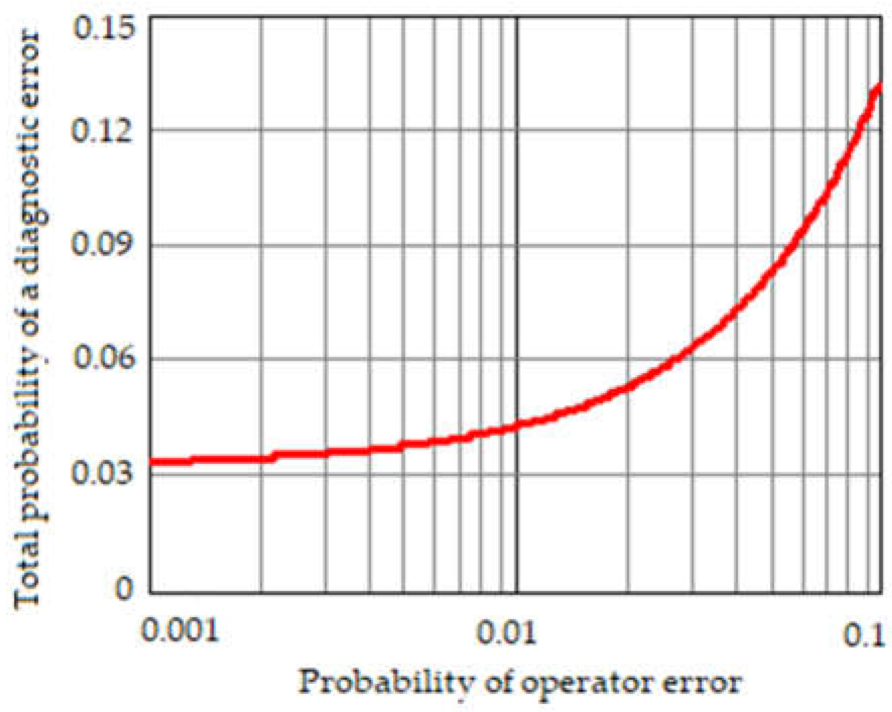
Figure 2.
A simulated example of crack depth growth curves.
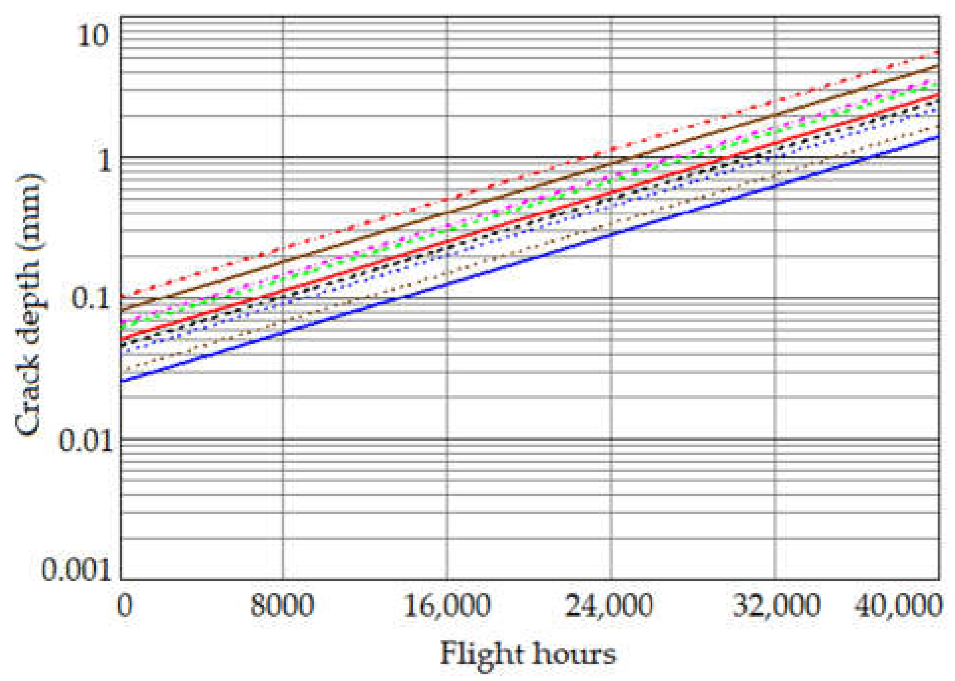
Figure 3.
The dependences of the probabilities of the true positive and reliability function (a), false negative (b), true negative and cumulative function (c), and false positive (d) versus the time of testing expressed in the number of flight hours when σe = 0.1 mm.
Figure 3.
The dependences of the probabilities of the true positive and reliability function (a), false negative (b), true negative and cumulative function (c), and false positive (d) versus the time of testing expressed in the number of flight hours when σe = 0.1 mm.
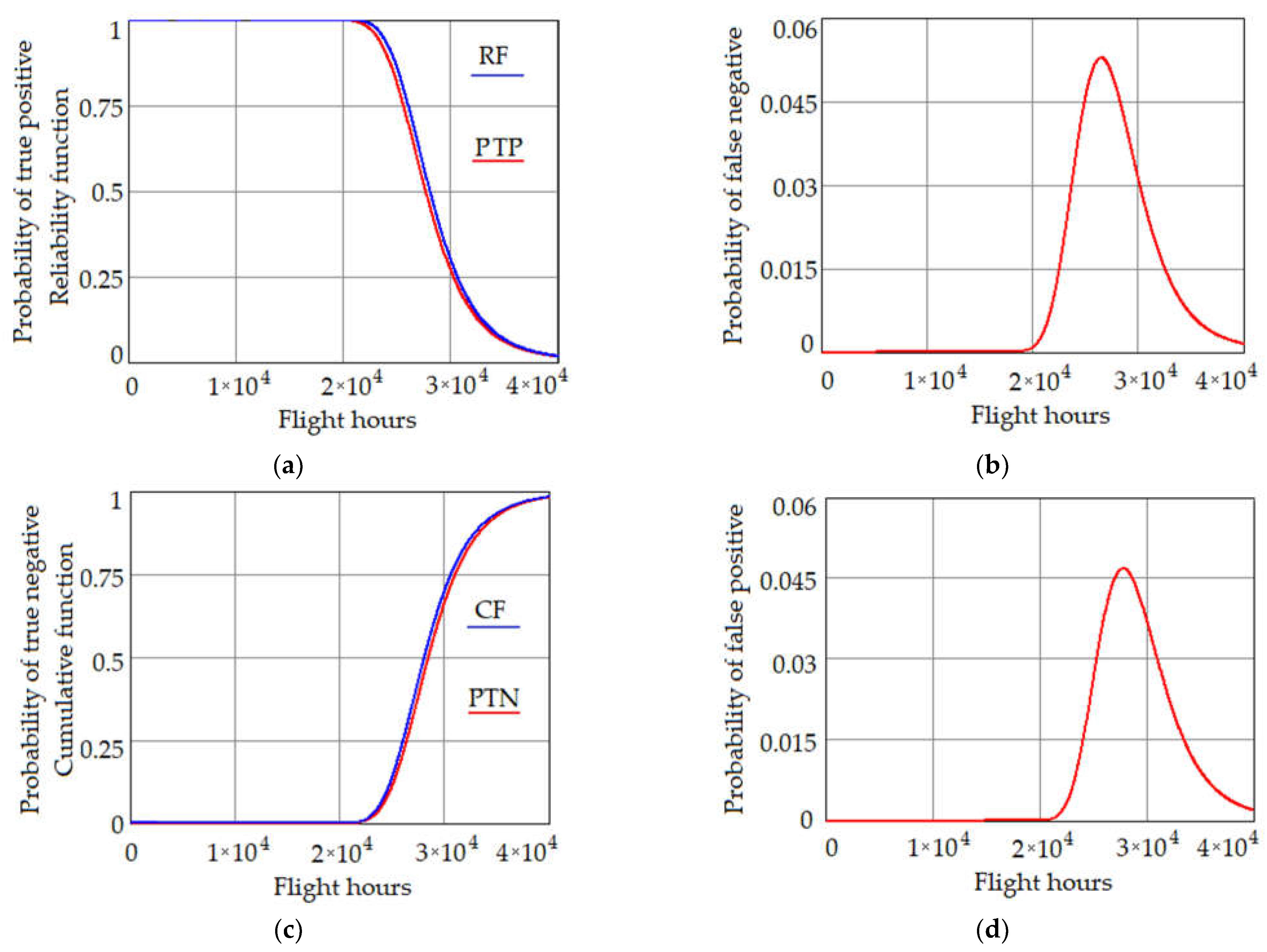
Figure 4.
The dependences of the probabilities of the true positive and reliability function (a), false negative (b), true negative and cumulative function (c), and false positive (d) versus the time of testing expressed in the number of flight hours when σe = 0.2 mm.
Figure 4.
The dependences of the probabilities of the true positive and reliability function (a), false negative (b), true negative and cumulative function (c), and false positive (d) versus the time of testing expressed in the number of flight hours when σe = 0.2 mm.
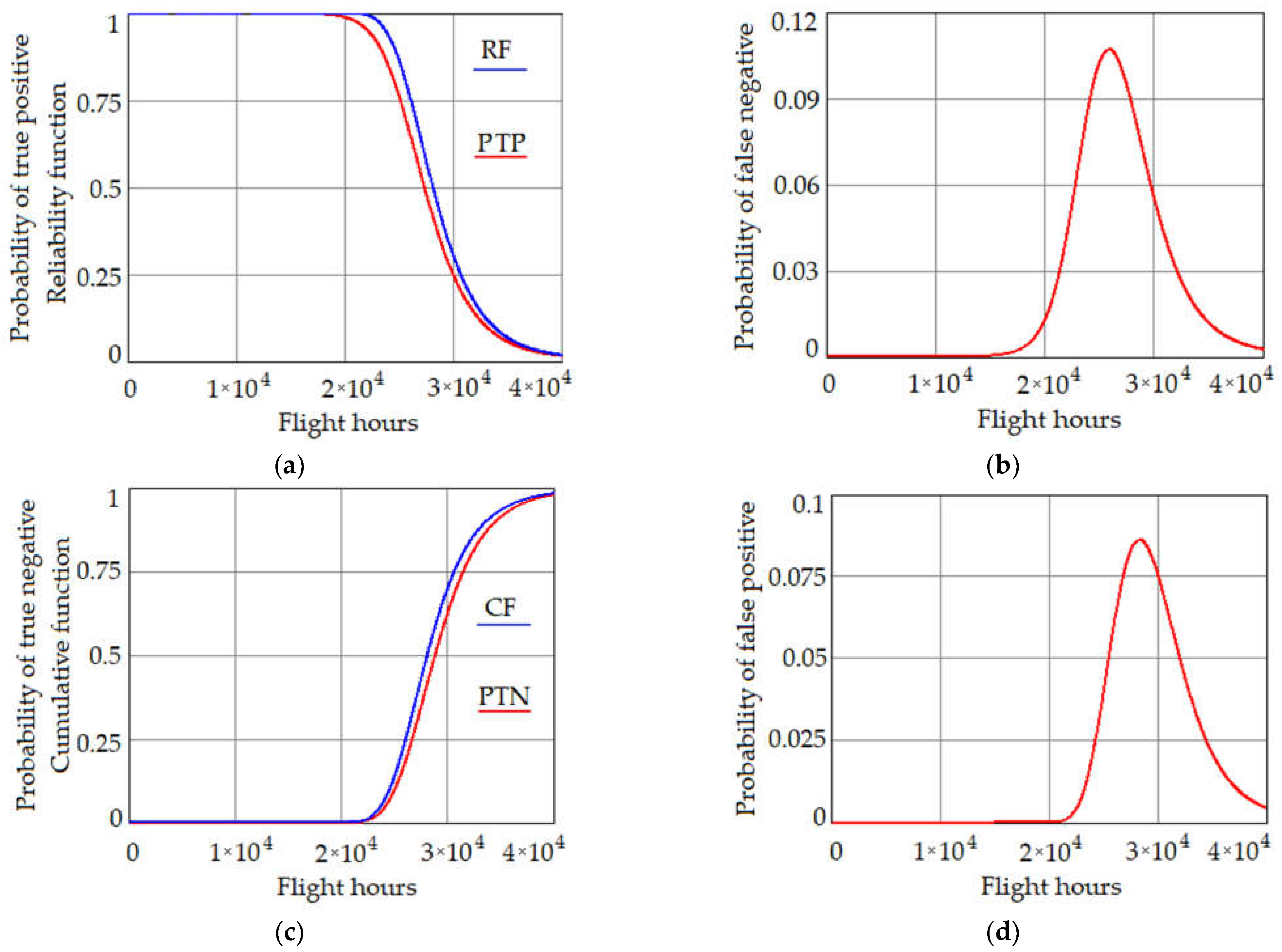
Figure 5.
The dependences of the probability of a diagnostic error versus the time of testing expressed in the number of flight hours when (a) Poe = 0 and σe = 0.1 mm (curve 1) and Poe = 0.001 and σe = 0.1 mm (curve 2), (b) Poe = 0 and σe = 0.1 mm (curve 1) and Poe = 0.1 and σe = 0.1 mm (curve 2), (c) Poe = 0 and σe = 0.2 mm (curve 1) and Poe = 0.001 and σe = 0.2 mm (curve 2), and (d) Poe = 0 and σe = 0.2 mm (curve 1) and Poe = 0.1 and σe = 0.2 mm (curve 2).


Table 1.
Input data.
| Object of Diagnostics | Diagnostic Parameter | Nominal Value | Lower and Upper Tolerance Limits | Standard Deviation | ||
|---|---|---|---|---|---|---|
| No. | Name | Nν | aν and bν | Diagnostic Parameter, σν | Measurement Error, σt,ν | |
| VHF communication system | 1 | Transmitter power, W | 20 | 16 | 1.79 | 0.55 |
| 2 | Receiver sensitivity, μV | 2.5 | 3 | 0.23 | 0.05 | |
| 3 | Modulation index, % | 92.5 | 85–100 | 3.48 | 0.35 | |
Table 2.
A priori probabilities of the system’s states.
| Name of Communication System’s State | Technical Condition of the Communication System | A Priori Probability of the System State P(Si) |
|---|---|---|
| S1 | 111 | 0.942 |
| S2 | 110 | |
| S3 | 101 | |
| S4 | 011 | |
| S5 | 100 | |
| S6 | 010 | |
| S7 | 001 | |
| S8 | 000 |
Table 3.
Probabilities of correct and incorrect decisions.
| Number of the DP No. | A Priori Probability That the ν DP Is within the Tolerance Range | A Priori Probability That the OD Is Operable P | Probability of a False Negative for the ν DP | Probability of a False Positive for the ν DP |
|---|---|---|---|---|
| 1 | 0.987 | 0.942 | 0.006335 | 0.002719 |
| 2 | 0.985 | 0.004430 | 0.002463 | |
| 3 | 0.969 | 0.003605 | 0.002749 |
Table 4.
A comparison of the calculated trustworthiness indicators of diagnosis with and without considering the characteristics of the reliability of the human operator and diagnostic tool.
Table 4.
A comparison of the calculated trustworthiness indicators of diagnosis with and without considering the characteristics of the reliability of the human operator and diagnostic tool.
| The Values of Reliability Characteristics of HO and DT | The Probabilities of Correct and Incorrect Decisions | |||||
|---|---|---|---|---|---|---|
| P(H1) = 0.98, P(H2) = 0.011, P(H3) = 0.009, P(D1) = 0.97, P(D2) = 0.01, P(D3) = 0.02 | 0.902 | 0.949 | ||||
| P(H1) = 1, P(H2) = P(H3) = 0, P(D1) = 1, P(D2) = P(D3) = 0, | 0.928 | 0.9779 | ||||
Disclaimer/Publisher’s Note: The statements, opinions and data contained in all publications are solely those of the individual author(s) and contributor(s) and not of MDPI and/or the editor(s). MDPI and/or the editor(s) disclaim responsibility for any injury to people or property resulting from any ideas, methods, instructions or products referred to in the content. |
© 2023 by the authors. Licensee MDPI, Basel, Switzerland. This article is an open access article distributed under the terms and conditions of the Creative Commons Attribution (CC BY) license (https://creativecommons.org/licenses/by/4.0/).
Share and Cite
MDPI and ACS Style
Ulansky, V.; Raza, A. Uncertainty Quantification of Imperfect Diagnostics. Aerospace 2023, 10, 233. https://doi.org/10.3390/aerospace10030233
AMA Style
Ulansky V, Raza A. Uncertainty Quantification of Imperfect Diagnostics. Aerospace. 2023; 10(3):233. https://doi.org/10.3390/aerospace10030233
Chicago/Turabian StyleUlansky, Vladimir, and Ahmed Raza. 2023. "Uncertainty Quantification of Imperfect Diagnostics" Aerospace 10, no. 3: 233. https://doi.org/10.3390/aerospace10030233
Note that from the first issue of 2016, this journal uses article numbers instead of page numbers. See further details here.