High Enthalpy Non-Equilibrium Expansion Effects in Turbulent Flow of the Conical Nozzle

Abstract

High enthalpy stagnation gas can be converted into hypervelocity flow through the contraction—expansion nozzle. The enthalpy flow in the nozzle can be divided into three regions: an equilibrium region, a non-equilibrium region, and a frozen region. The stagnation gas with a total enthalpy of 13.4 MJ/kg is used to analyze the thermochemical non-equilibrium effects. At the selected conditions, the effects of a conical nozzle under different expansion angles of the expansion section, curvature radius of the throat, throat radius, and convergence angle of the convergent section are investigated. Based on the Spalart–Allmaras one-equation turbulence model with the Catris–Aupiox compressibility correction, a multi-block solver for axisymmetric compressible Navier–Stokes equations is applied to simulate the thermochemical non-equilibrium flow in several high enthalpy conical nozzles. The multi-species two-temperature equation is employed in the calculation. The results reveal three interesting characteristics: Firstly, the thermochemical non-equilibrium effects are sensitive to the maximum expansion angle and throat radius but not to the radius of throat curvature and contraction angle. Secondly, as the maximum expansion angle decreases and the throat radius increases, the flow approaches equilibrium state. When the maximum expansion angle decreases from 12° to 4°, the freezing temperature decreases from 2623 K to 2018 K. When the throat diameter increased from 10 mm to 30 mm, the freezing temperature decreased from 2442 K to 2140 K. Finally, the maximum expansion angle and throat radius not only affect the position of the freezing point but also the flow field parameters, such as temperature, Mach number, and species mass fraction.

1. Introduction

When a spacecraft reenters Earth’s atmosphere or enters the interplanetary atmosphere, the flow surrounding the aircraft is characterized by high-temperature effects, such as the dissociation and even ionization of the fluid molecules flowing with hypersonic vehicles [1,2,3,4]. The high enthalpy tunnel can duplicate the high flow velocities and, subsequently, the high-temperature effects [5,6]. For the high enthalpy shock tunnel, the stagnation gas passes through a convergent–divergent nozzle and transforms into the hypervelocity free flow, where the stagnation gas is highly dissociated [6,7]. During the nozzle expansion, the velocity of the airflow increases rapidly, but the temperature and density of the airflow decrease rapidly. The flow cannot reach the equilibrium state under the local temperature and pressure, and it tends to be thermochemically frozen not far away from the throat [7,8]. The vibrational relaxation and recombination reaction cannot return it to the natural atmospheric state. At the nozzle exit, the vibrational temperature of the airflow is very different from the translational temperature, and the chemical species do not reach the natural atmospheric level. In other words, the free flow of the high-enthalpy wind tunnel has a certain degree of thermochemical non-equilibrium [9,10,11]. This situation is undesirable, as it makes the test data of the nozzle exit airflow inconsistent with the flight environment, which can restrict the ability to simulate the high enthalpy nozzle. Therefore, it is necessary to reduce the thermochemical non-equilibrium flow of the high enthalpy nozzle.

There are many high enthalpy shock tunnels in the world, such as T4 [12], T5 [13], HIEST [14], HEG [15], LENS I [16], T6 [17], JF-10 [18], and FD-21 [19]. The high enthalpy nozzles of these tunnels can be divided into two categories: contour nozzles and conical nozzles. The high enthalpy nozzles have different maximum expansion angles (MEAs), ranging from 4° to 12°. If the MEA is too small, the nozzle is too long, resulting in high costs. When the MEA is too large, the flow separation downstream of the throat is more easily caused, which affects the quality of the flow field. Several studies have been conducted on the high enthalpy nozzles themselves [7,8,9], but only few of them focused on the thermochemical non-equilibrium expansion effects based on different MEAs. Therefore, it is necessary to analyze the influence of MEA and other design parameters on the nozzle, such as the throat curvature radius (TCR), the throat radius (TR), and the convergence angle (CA) on the nozzle. Numerous factors must be considered when designing a high enthalpy contour nozzle. Unreasonable design parameters can lead to a large error [9,15,20]. Conical nozzles have fewer design parameters and are easier to design. Therefore, conical nozzles are suitable for studying the thermochemical non-equilibrium expansion effects.

To improve the quality of the flow field at the outlet of the high enthalpy nozzle, some geometric design parameters are discussed, including MEA, TCR, TR, and CA. MEA is a key parameter in the design of the nozzle expansion section, which determines the length of the nozzle and the expansion process of the airflow. TCR is the curve connecting the contraction section and expansion section of the nozzle, where the airflow changes from subsonic to supersonic in this area. TR is the nozzle throat, which determines parameters such as nozzle outlet pressure and Mach number. CA determines the length of the contraction section. The five-species model (O₂, N₂, NO, O, N) and seven-species model (O₂, N₂, NO, O, N, NO+, e−) are used to calculate the high enthalpy flow field in this paper. The axisymmetric compressible Navier–Stokes equations with Park’s two-temperature model [21] are solved with a multi-block finite volume method. The conical nozzle of the FD-21 wind tunnel is used as the research object. By comparing the nozzles under different parameters, it is concluded that a small MEA and a large TR can effectively suppress the thermochemical non-equilibrium effects, but the TCR and CA have a minor influence on non-equilibrium flow. Considering the cost and expansion effects, the MEA of FD-21 wind tunnel conical nozzle is 9°, throat diameter is 0.02 m, nozzle outlet diameter is 2 m, contraction angle is 30°, and the inlet diameter of the contraction section is 0.29 m. These results can serve as a useful reference for the design of high enthalpy conical nozzles, especially high enthalpy contour nozzles.

2. Numerical Methods

2.1. Governing Equations

In the present study, the thermochemical non-equilibrium flow calculation program developed by our research group was used to numerically simulate the nozzle flow field, and the internal flow field characteristics were calculated [7]. The unsteady, dimensionless, axisymmetric, compressible Navier–Stokes equation was employed for the viscous case. For multi-species air in thermochemical non-equilibrium state [22,23,24], this Navier–Stokes equation can be expressed in the vector equation [25] as:

$$\frac{\partial U}{\partial t}+\frac{\partial F}{\partial x}+\frac{\partial G}{\partial r}+M=\frac{1}{Re}\left(\frac{\partial F_v}{\partial x}+\frac{\partial G_v}{\partial r}+M_v\right)+W$$

(1)

where U is a vector of conservative quantities, F and G represent the convective fluxes, and F_V and G_V are the transport terms, respectively. M and M_V are the inviscid and viscous source terms, respectively. W represents the chemical and vibrational terms. Re is the Reynolds number. These quantities are expressed as follows:

$$U={\left[\rho C_i\left(i=1,\dots ,ns\right),\rho u,\rho v,\rho E,\rho e_V\right]}^T$$

(2)

$$F={\left[\rho u{C}_i\left(i=1,\dots ,ns\right),\rho u^2+p,\rho uv,\rho uH,\rho u{e}_V\right]}^T$$

(3)

$$G={\left[\rho v{C}_i\left(i=1,\dots ,ns\right),\rho uv,\rho v^2+p,\rho vH,\rho v{e}_V\right]}^T$$

(4)

$$M=\frac{1}{r}{\left[\rho v{C}_i\left(i=1,\dots ,ns\right),\rho uv,\rho v^2,\rho vH,\rho v{e}_V\right]}^T$$

(5)

$$F_v={\left[\frac{L{e}_{i}k}{Pr{C}_p}\frac{\partial C_i}{\partial x}\left(i=1,\dots ,ns\right),{\tau }_{xx},{\tau }_{xr},u{\tau }_{xx}+v{\tau }_{xr}+q_x,q_{vx}\right]}^T$$

(6)

$$G_v={\left[\frac{L{e}_{i}k}{Pr{C}_p}\frac{\partial C_i}{\partial r}\left(i=1,\dots ,ns\right),{\tau }_{xr},{\tau }_{rr},u{\tau }_{xr}+v{\tau }_{rr}+q_r,q_{vr}\right]}^T$$

(7)

$$M_v=\frac{1}{r}{\left[\frac{L{e}_{i}k}{Pr{C}_p}\frac{\partial C_i}{\partial r}\left(i=1,\dots ,ns\right),{\tau }_{xr},{\tau }_{rr}-{\tau }_{\theta \theta },u{\tau }_{xr}+v{\tau }_{rr}+q_r,q_{vr}\right]}^T$$

(8)

$$W={\left[{\dot{w}}_i\left(i=1,\dots ,ns\right),0,0,0,S_v\right]}^T$$

(9)

where ns is 7 or 5, which is the number of species. ρ and p are the density and pressure of the mixture, respectively. C_i is the species mass fraction. u and v are the components of the velocity V in the axial and radial direction. x and r are the coordinates in the axial and radial direction, respectively. Le_i is the Lewis number of the species. P_r and C_p are the Prandtl number and specific heat of the mixture, respectively. k is the coefficient of heat conduction. Sv is the vibrational source terms of the species. w_i is the chemical source term. H is total enthalpy.

The components of the viscous stress tensor τ are as follows

$${\tau }_{xx}=-\frac{2\mu }{3}\nabla \cdot \overrightarrow{v}+2\mu \frac{\partial u}{\partial x}$$

(10)

$${\tau }_{rr}=-\frac{2\mu }{3}\nabla \cdot \overrightarrow{v}+2\mu \frac{\partial u}{\partial r}$$

(11)

$${\tau }_{\theta \theta }=-\frac{2\mu }{3}\nabla \cdot \overrightarrow{v}+2\mu \frac{v}{r}$$

(12)

$${\tau }_{xr}={\tau }_{rx}=\mu \left(\frac{\partial u}{\partial r}+\frac{\partial v}{\partial x}\right)$$

(13)

where the divergence of the velocity is represented by the following:

$$\nabla \cdot \stackrel{\rightharpoonup }{v}=\frac{\partial u}{\partial x}+\frac{\partial v}{\partial r}+\frac{v}{r}$$

(14)

The total enthalpy H is expressed as follows:

$$H=E+\frac{p}{\rho }$$

(15)

where E is the total energy per unit volume, including translational energy e_t, rotational energy er, vibrational energy e_V, electronic energy e_e, free energy e₀, and the kinetic energy of the gas V²/2. E is defined as follows:

$$E={\displaystyle \sum _{i=1}^{ns}{C}_i\left(e_{ti}+e_{ri}+e_{ei}+e_{0i}\right)+{\displaystyle \sum _{i=1}^{ns}{C}_i{e}_{vi}\left(T_v\right)+\frac{1}{2}}}{V}^2$$

(16)

where nt is the number of species that do not have electrons in ns. q_x, q_r, q_vx, and q_vr are the components of the total heat flow. They are expressed as follows:

$$\left\{\begin{array}{l}{q}_n=\frac{1}{Pr}\left(k_t\frac{\partial T}{\partial n}+k_v\frac{\partial T_v}{\partial n}+{\displaystyle \sum _{i=1}^{ns}{h}_i\frac{L{e}_{i}k}{C_p}\frac{\partial C_i}{\partial n}}\right)\\ q_{vn}=\frac{1}{Pr}\left(k_v\frac{\partial T_v}{\partial n}+{\displaystyle \sum _{i=1}^{n\mathrm{s}}{e}_{vi}\frac{L{e}_{i}k}{C_p}\frac{\partial C_i}{\partial n}}\right)\begin{array}{cc}& \left(n=x,r\right)\end{array}\end{array}\right.$$

(17)

Here, S_V is expressed as follows:

$$S_v=\rho \frac{e_v\left(T\right)-e_v\left(T_v\right)}{{\tau }_v}+{\displaystyle \sum _{i=1}^{ns}\dot{w}{e}_{vi}}$$

(18)

2.2. Non-Equilibrium Model

Each species of the mixture was considered a perfect gas. The chemical source terms were derived from several reactions. The following equations were derived for the five-species and seven-species air models with a reaction mechanism consisting of several reversible chemical steps [26].

$$7-species\left\{\begin{array}{l}5-species\left\{\begin{array}{l}{\mathrm{O}}_2+M_1\iff 2\mathrm{O}+M_1\\ N_2+M_2\iff 2N+M_2\\ \mathrm{NO}+M_3\iff N+O+M_3\\ NO+O\iff N+O_2\\ N_2+O\iff NO+O\end{array}\right.\\ \mathrm{NO}+M_4\iff N{O}^{+}+e^{-}+M_4\\ N+O\iff N{O}^{+}+e^{-}\\ N_2+O_2\iff NO+{\mathrm{NO}}^{+}+e^{-}\end{array}\right.$$

(19)

where M₁ = N, O, NO, N₂ and O₂; M₂ = N, O, NO, N₂ and O₂; M₃ = N, O, NO, N₂ and O₂; M₄ = N₂ and O₂.

The coupling between chemical processes and vibrational processes had to be considered. The forward reaction rate k_f,r, and backward reaction rate k_b,r of the dissociation equations were expressed in the modified Arrhenius form [25] as follows:

$$k_{f,r}=A_{f,r}{T}_{av}^{B_{f,r}}\exp \left(-T_{D_{f,r}}/T{}_{av}\right)$$

(20)

$$k_{b,r}=A_{b,r}{T}_{tr}^{B_{b,r}}\exp \left(-T_{D_{b,r}}/T\right)$$

(21)

where A_f,r and A_b,f are the forward and backward reaction rate constants. T_Df,r and T_Db,r are the characteristic reaction temperatures for forward and backward reactions. The values of the reaction rates, k_f,r and k_b,r, are derived from reference [25] for the multi-species air model. For dissociative reactions, the geometric average temperature was assumed to be T_av, which is defined as an average of the translational temperature T and vibrational temperature T_v, which is expressed as follows [21]:

$$T_{av}=\sqrt{T{T}_{\mathrm{v}}}$$

(22)

With regard to radiative energy flux, Park’s relation for T_av has shown a good agreement with experimental results [27].

The viscosity and thermal conductivity of the mixture were calculated by Gupta–Yos viscosity curve fits [25] for each species.

$${\mu }_s=\exp \left(C_{\mu ,s}\right)T^{\left(A_{\mu ,s}\ln T+B_{\mu ,s}\right)}$$

(23)

$$k_s=\exp \left(E_{k,s}\right)T^{\left(A_{k,s}{\left(\ln T\right)}^3+B_{k,s}{\left(\ln T\right)}^2+C_{k,s}\left(\ln T\right)+D_{k,s}\right)}$$

(24)

where A_μ,s, B_μ,s, C_μ,s, A_k,s, B_k,s, C_k,s, D_k,s, and E_k,s are constants. Wilke’s Law [28] was used to calculate the bulk quantities.

When the temperature was between 300 K and 8000 K, the vibrational relaxation time τi was given by the following equation [28].

$${\tau }_i={\tau }_{i,MW}+{\tau }_{i,P}$$

(25)

where τ_i,P is translational-vibrational energy relaxation time (TVERT) of the species, as reported by Park [27]. τ_i,MW is the TVERT for the molecular species s, and it is adjusted based on the study of Millikan and White [28].

$$P{\tau }_{i,MW}=\frac{{\displaystyle \sum _{i=1}^{ns}{N}_i\exp \left[A_s\left(T^{-1/3}-0.015M_{si}^{0.25}\right)-18.42\right]}}{{\displaystyle \sum _{i=1}^{ns}{N}_i}}$$

(26)

where P is the pressure, N_i is the number density, M_si is reduced molecular weight of species, and A_s is a constant.

For a perfect gas, the expression for the speed of sound is given as $a^2\equiv {\left(\partial p/\partial \rho \right)}_S$. The corresponding expressions of non-equilibrium sound speed a_n and the frozen sound speed a_f can be expressed as

$$a_n^2=-{\left[\left(\frac{\rho h_p-1}{\rho h_p}\right)+\frac{1}{\rho u{h}_{\rho }\left(\frac{\partial p}{\partial r}\right)}{\displaystyle \sum _i^{ns}{h}_{Ci}{w}_i}\right]}^{-1}$$

(27)

$$a_f^2=-{\left[\left(\frac{\rho h_p-1}{\rho h_p}\right)\right]}^{-1}$$

(28)

The unsteady flow field equations of the axisymmetric nozzle with given stagnation and wall conditions were integrated in time. The time-step size was 1.0 × 10⁻⁶ s, and the Number of time steps was less than 5000. Jameson’s fourth-order Runge–Kutta method [29] was used for the time integration. The low-dissipation advection upwind splitting method (AUSM) [30] was used to calculate the inviscid numerical fluxes, and the monotonic upstream-centered scheme for conservation law (MUSCL) was used for third-order spatial accuracy.

For the strong favorable pressure gradient around the nozzle throat, Candler [31] and Wang [32] calculated the typical hypersonic nozzle flows. The calculated results based on the Spalart–Allmaras one-equation turbulence model [33] with the Catris–Aupiox compressibility correction were in good agreement with the measured nozzle flow field. Under the condition of divergent free flow, the outflow boundary is dominated by hypersonic flow. All the conservative variables were extrapolated. A solid wall was used without slip condition. The wall conditions were given for a fully catalytic wall and an isothermal wall where T_w = 300 K.

2.3. Physical Model and Grid Generation

As mentioned above, the T5 nozzle [13], the HEG nozzle [15], and the FD-21 nozzle [19] were studied. The T5 nozzle and HEG nozzle were examined to verify the accuracy of the calculation method. Based on the FD-21 nozzle, the thermochemical non-equilibrium expansion effects were studied by changing the MEA of the expansion part, TCR, TR, and CA of the convergent part.

For the conical nozzles, the main parameters, including CA θ_c, TCR r_c, TR r_t, exit radius (r_e), MEA θ_e, and expansion ratio (ER) are listed in

Table 1. Geometrical parameters of reference nozzles.

Case	rc (mm)	θc (°)	θe (°)	rt (mm)	re (mm)	L (m)	ER
T5	45	20	7	15	150	1.2	100
HEG	11.0	30	6.5	5.5	440	3.75	1600

and

Table 2. Geometrical parameters based on the FD-21 nozzle.

Case	θc (°)	rc (mm)	θe (°)	rt (mm)	L (m)	ER
1	30	20	4.0	10	14.43	10,000
2	30	20	6.5	10	9.01	10,000
3	30	20	9.0	10	6.52	10,000
4	30	20	12.0	10	4.91	10,000
5	30	20	9.0	20	6.32	2500
6	30	20	9.0	30	6.38	1111
7	20	20	9.0	10	6.63	10,000
8	45	20	9.0	10	6.40	10,000
9	30	10	9.0	10	6.50	10,000
10	30	40	9.0	10	6.49	10,000

. The parameters of the T5 nozzle and the HEG nozzle are shown in Table 1. Table 2 shows a total of 10 cases. Cases 1 to 4 were used to verify the effect of the MEA θ_e. Cases 3, 5, and 6 were used to verify the influence of changes in TR r_t on the thermochemical non-equilibrium effects. Cases 3, 7, and 8 were used to verify the influence of changes in CA θ_c on the thermochemical non-equilibrium effects. Cases 3, 9, and 10 were used to verify the influence of the change of TCR r_c on the thermochemical non-equilibrium effects. For all the cases based on the FD-21 nozzle, the inlet radius was 145 mm and the exit radius was 1000 mm.

A structured grid was used for all the numerical simulations, and the structured grid is shown in Figure 1. The grid consisted of two blocks: the first block was the shock tube part, which was 300 mm away from the end of the shock tube, and the other was the nozzle part. The total number of grids was 168,000. The shock tube part included 51 × 161 grids, and the nozzle part contained 1000 × 161 grids. The system was used with Δx_min = 1 × 10⁻⁴ m located at the throat section, and Δy_min = 2 × 10⁻⁸ m at the wall. Exponential compression was used in the radial direction. A grid convergence study was conducted with three different grid resolutions (79,775, 150,120, and 317,100), and a small change in pressure, species fraction, velocity, and Mach number distribution was registered. For each grid system, the y+ value was less than one.

2.4. Conditions of Numerical Simulation

The initial conditions were chosen from the data obtained by the T5 [13] and HEG [15] nozzle, which correspond to Case1 and Case2 in

Table 3. Initial conditions.

Case	P0 (MPa)	T0 (K)	h0 (MJ/kg)	CN2 (%)	CO2 (%)	CNO (%)	CN (%)	CO (%)	CNO+ (%)
1	20.7	6359	11.3	0.7059	0.0234	0.1000	0.0013	0.1579	9.96E−5
2	48.3	7410	13.4	0.6872	0.0150	0.9880	0.3200	0.1670	0.01

, respectively. The pressure, temperature, and species fraction in reservoir conditions were obtained by equilibrium assumption and are listed in Table 3. Heat flux is an important parameter [34], but this paper focuses on the nozzle uniformity parameter. The wall boundary conditions have a negligible effect on the uniform zone of nozzle [35].

3. Verification of Calculation Procedure

3.1. Precision Estimates

For the large-scale simulation of gas dynamics of complex chemical reactions, it was necessary to estimate the accumulated accuracy and error [36]. There was a certain amount of error at each step of the integration, which depended on the spatial resolution as well as the numerical solver. This error can be expressed in absolute or relative values. Error was accumulated in successive time steps [7].

In the one-dimensional case, the relative error S₁ is proportional to the average ratio of the cell size ΔL to the field size L₁ in the direction of the power integration, depending on the scheme precision [37]:

$$S_1\approx {\left(\frac{\Delta L}{L_1}\right)}^{k+1}$$

(29)

where k is the order of the numerical scheme accuracy. When there are several directions in the synthesis, the errors [37] are written as

$$S_{error}\approx {\displaystyle \sum _{i=1}^2{S}_i}$$

(30)

The allowable value of total error Smax [37] is defined by the simulator user. Since the initial and boundary conditions are usually not known with a high degree of accuracy, Smax was between 1% and 5%. The following inequality was satisfied as follows:

$$S_{error}·\sqrt{n}\le S_{\max }$$

(31)

where n is the number of time steps in Navier–Stokes integral equations.

Another important feature was introduced for the results of the supercomputer simulation. The ratio of the maximum allowable time steps to the actual time steps [37] can be defined as follows:

$$R_s=n_{\max }/n$$

(32)

Table 4. Error estimates.

Case	T5	HEG
Allowable error	5%	5%
Grid resolution	1051 × 161	1051 × 161
Physical time simulated(ms)	4.0	5.0
Number of time steps	4000	5000
Accumulated error	2.40 × 10−7	2.40 × 10−7

shows the accumulated error for grid resolution and physical time simulation [7]. It was assumed that the allowable error was 5% because the initial and boundary conditions are usually not known with a high degree of accuracy [36]. For the present numerical simulation, the results are highly reliable but are not always suitable for simulating longer step sizes.

3.2. Verification of the Calculation Method

The 5-species 2-temperature (5S2T) model and the 7-species 2-temperature (7S2T) model were used to calculate the flow field of the T5 and HEG nozzles. For the T5 and HEG nozzles, the initial condition was based on Case 1 and Case 2 in Table 3, respectively. Figure 2 shows the comparison of the distribution of species mass fraction in the flow field [13], using the same 5-species 2-temperature model as the reference.

Table 5. Comparison of flow parameters in the T5 nozzle.

Results	P∞ (Pa)	U∞ (m/s)	CN2	Co2	CNO	CO	CN
T5	1150	--	0.7414	0.1692	0.05135	0.0388	1.12 × 10−4
7S2T	1208	4135	0.7419	0.1678	0.05015	0.0401	9.95 × 10−5
5S2T	1250	4128	0.7411	0.1662	0.05174	0.0408	9.98 × 10−5

and

Table 6. Comparison of flow parameters in the HEG nozzle.

Results	P∞ (Pa)	T∞ (K)	U∞ (m/s)	CN2	Co2	CNO	CO	CN
HEG	713	694	4776	73.56	13.40	5.09	7.96	1.0 × 10−8
5S2T	705	720	4823	0.73.94	13.48	5.03	7.83	1.8 × 10−8
7S2T	701	723	4842	0.74.01	13.75	4.96	7.25	1.4 × 10−7

show a comparison of the pressure and species mass fraction at the exit of the T5 and HEG nozzles. It is clear that the calculation results for the T5 and HEG nozzles are in good agreement with the reference values [13,15]. Compared to 5-species ions, the 7-species ions belong to the micro-species. Under the aforementioned conditions, the proportion of NO+ and e- in the mass of 7-species ions was less than 0.03% of the total mass compared to 5-species ions. The chemical energy of the micro-species was negligible relative to the total gas flow, so they did not affect the main flow and thermochemical parameters. This phenomenon is consistent with previous research results.

The discrepancy between the calculated and reference values is usually 5% or less for all of the cases considered. There are three main reasons [7] for these differences: First, the vibrational modeling modifies the translational temperature, as deduced from Equation (16). Second, there are the different expressions of the transport coefficients. The species e- and NO+ belong to the micro-species. The results verify the positive determination of the relevant parameter settings and the accuracy of the procedure. Third, the turbulence energy can decrease some other energy in an isolated system. When the total temperature exceeds 6000 K, there are trace species such as e-, NO+. Therefore, it was deemed more appropriate to use the 7-species model, so it was employed for further analysis.

4. Results and Discussion

The different geometries in Table 2, which are based on the FD-21 nozzle, were evaluated. The reservoir conditions for Case 2 are listed in Table 3.

4.1. Freezing Point Position

A comparison of Cases 1, 2 3, and 4 reveal the influence of the MEA θ_e on the thermochemical non-equilibrium effects. The translational temperature T and vibrational temperature T_v of the nozzle centerline are shown in Figure 3. It can be seen that the vibrational temperature T_v and the translational temperature T are the same before the throat, and the gas is in the thermodynamic equilibrium state. After passing through the throat at x = 0 m, T_v and T begin to differ, and the non-equilibrium vibrational phenomenon occurs. Then, as the gas velocity gradually increases, the vibrational temperature becomes constant (freezing point). Not far from the downstream of the nozzle throat, the larger MEA of the nozzle corresponds to a higher vibrational temperature but slightly lower translational temperature. The MEAs were 4°, 6.5°, 9°, and 12°, and the freezing temperatures were 2018 K, 2113 K, 2442 K, and 2623 K, respectively. The distances x_f from the freezing point to the throat were 3.071, 1.576, 0.717, and 0.473 m. The freezing point diameters d_f of the corresponding nozzles were 0.438, 0.376, 0.254, and 0.220 m. The ratio df/dt of the freezing point diameter to the throat diameter was 21.9, 18.8, 12.7, and 11, respectively. The freezing point approaches the nozzle throat as the MEA increases. These phenomena can be explained as follows:

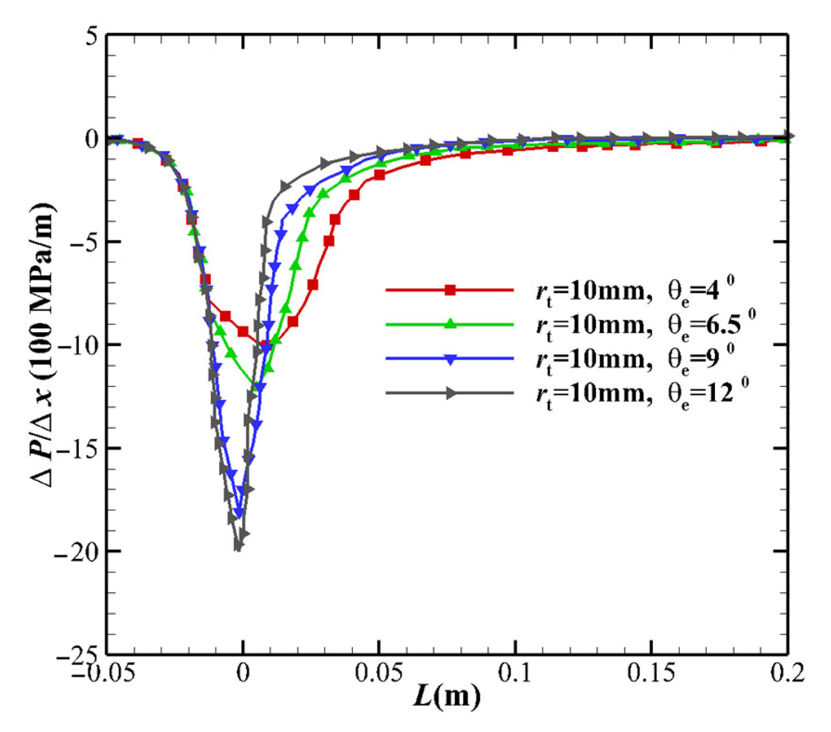
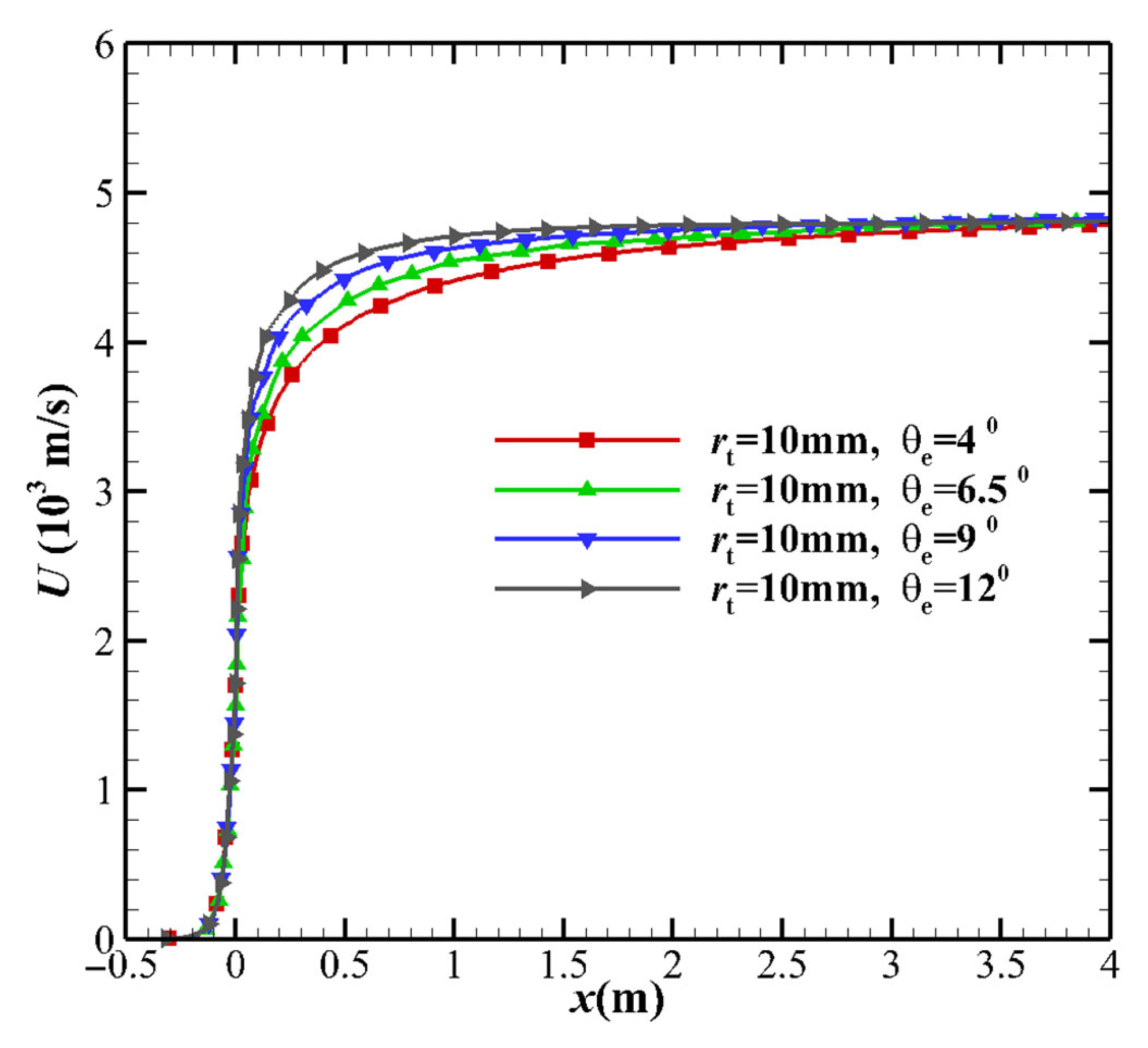
• As the MEA increases, the pressure gradient near the throat increases (see Figure 4), resulting in an increase in flow speed, as illustrated in Figure 5. As the pressure gradient increases, the pressure downstream of the throat decreases, which increases the TVERT, as deduced from Equation (25). Additionally, the increase in pressure gradient causes an increase in the flow velocity but a decrease in the flow time. Both shorten the transition from equilibrium to freezing, and the flow becomes close to the non-equilibrium flow.
• The pressure p decreases with the increase in the MEA. According to the ideal gas law p = nkT, the translational temperature is directly related to the pressure p, and the vibrational degree of freedom has no direct influence on the pressure. Therefore, the influence of the non-equilibrium on the pressure distribution is consistent with the trend of the influence on the translational temperature T.
• Not far from the downstream of the nozzle throat, the larger MEAθ_e corresponds to a slightly larger vibrational temperature, resulting in a higher vibrational energy level. The vibrational model modifies the translational temperature, as deduced from the kinetic energy in Equation (16). Due to the freezing of vibrational energy, the increase in the kinetic energy of the airflow in the nozzle mainly originates from the translational energy, which leads to a decrease in the translational temperature T. Since the vibration energy is frozen, it can also be determined that the contribution of vibrational energy to the speed is extremely small, which means that the non-equilibrium effect has almost no effect on the velocity u of the nozzle outlet. The velocity u is almost the same, which is consistent with h ≈ u²/2, and the velocity u is only related to the total enthalpy h of the nozzle stagnation gas.

The thermochemical non-equilibrium scale effects were studied by changing the TR r_t. Cases 3, 5, and 6 in Table 2 were selected, and the translational temperature T and vibrational temperature T_v are shown in Figure 6. In the downstream of the throat, the vibrational temperature and translational temperature are different. The separation point of the nozzle is also different. With the increase in the TR, the separation point and freezing point gradually move to the downstream of the nozzle. For the TR of 10, 20, and 30 mm, the freezing temperatures were 2442, 2207, and 2140 K, respectively. The distances xf from the freezing point to the throat were 0.717, 1.568, and 3.030 m. The freezing point diameters df of the corresponding nozzles were 0.254, 0.536, and 1.018 m. The ratio df/dt of the freezing point diameter to the throat diameter was 12.7, 13.4, and 16.9, respectively. As the TR increases, the freezing point moves away from the throat. These results can be explained in terms of the following.

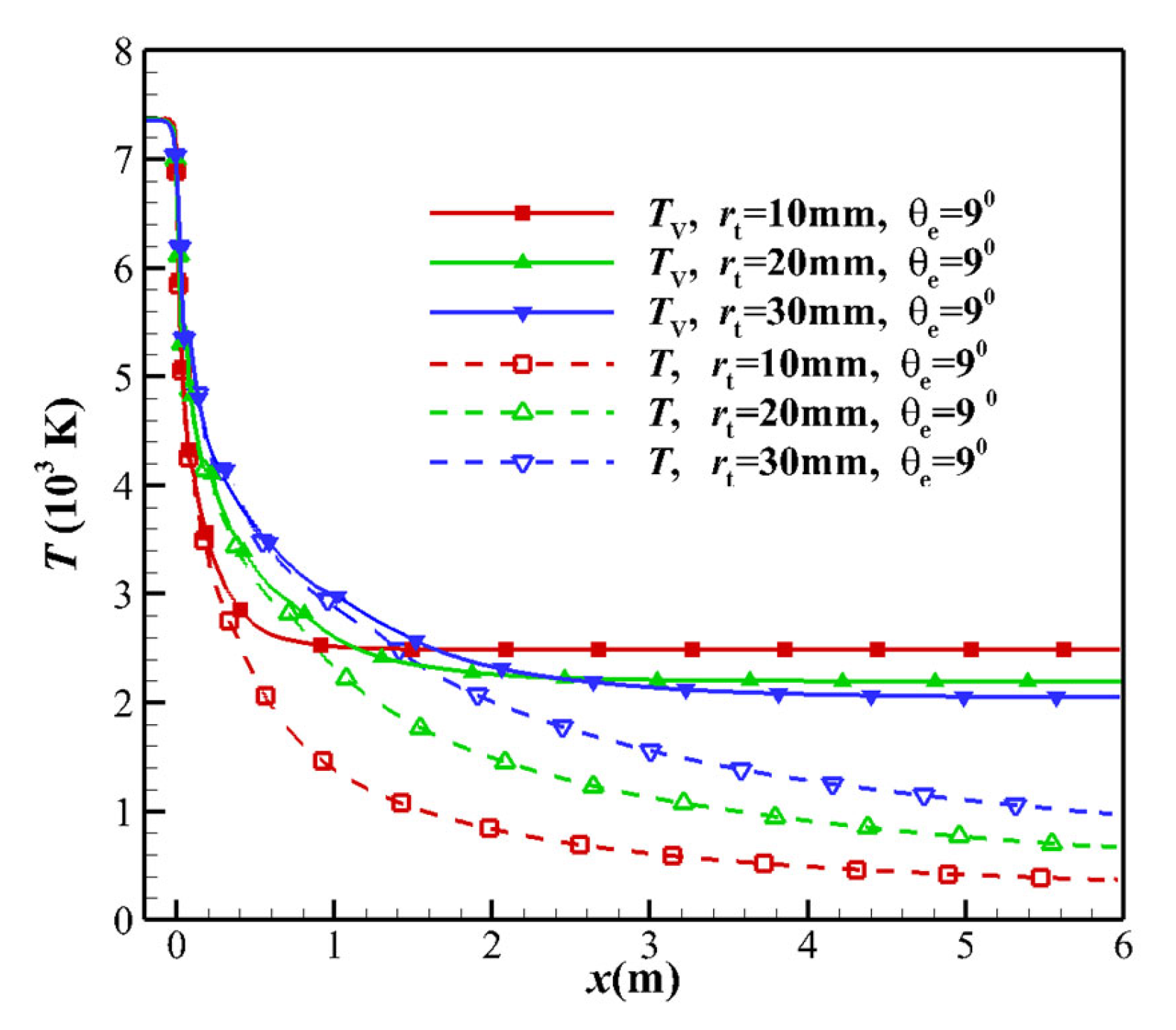
• As the TR increases, the pressure gradient near the throat decreases (see Figure 7), which raises the pressure downstream of the throat, causing a decrease in the TVERT, as deduced from Equation (26). Additionally, as the TR increases, the velocity near the throat decreases and the flow time increases. The overall effect is that the freezing point is far from the throat, and the flow state is close to the equilibrium state.
• For the equilibrium flow, the flow parameters on any cross-section are determined only by the nozzle stagnation conditions and the local area ratio. The throat at x = 0 mm and the throat upstream exhibit equilibrium flow, and the translational temperature and the vibrational temperature are not separated, as shown in Figure 7.
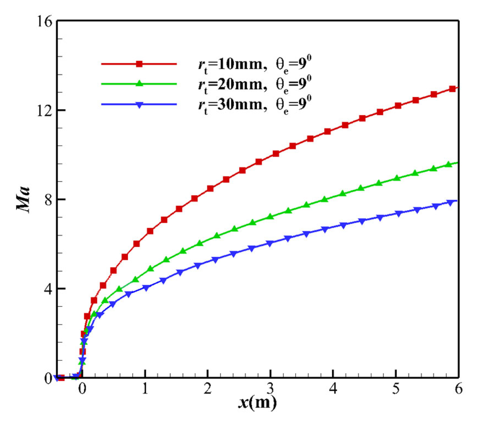
• The increase in the kinetic energy of the equilibrium flow originates from the translational kinetic energy and vibrational energy. Since the vibrational energy of the non-equilibrium flow freezes, the increase in the kinetic energy can only be attributed to the translational energy. As the TR increases, the velocity u at the throat decreases. The velocity u of the nozzle outlet is only related to the total enthalpy h of the nozzle stagnation gas, and the nozzle outlet velocity is almost the same (see Figure 8).

The contraction section and the throat were upstream of the freezing point of the high enthalpy nozzle. The CA θ_c and TCR r_c were varied to investigate the thermochemical non-equilibrium effect. In the subsonic region upstream of the throat, the flow is the equilibrium state. The variation of nozzle geometry in the equilibrium flow area has almost no impact on the non-equilibrium effect of the flow field. Cases 3, 7, and 8 in Table 2 were selected to study the influence of CA on the non-equilibrium effects. The freezing position and vibrational temperature of the flow field are almost unchanged (see Figure 9). The change in the TCR has a minor impact on the non-equilibrium effect, and the freezing position and vibrational temperature of the flow field are almost unchanged. The calculation results of cases 3, 9, and 10 are shown in Figure 10. As the airflow passes through the throat, the non-equilibrium effects begin to increase, and the flow freezes quickly downstream of the throat.

4.2. Mach Number

Although the high enthalpy nozzle is mainly used to simulate the speed and pressure of the flying objects, the Mach number is also a key parameter. It has been proved that changes in the MEA and TR can influence the non-equilibrium effect. Now, we discuss the effects of changes in the MEA and TR on the Mach number.

To study the influence of the MEA on the Mach number, cases 1, 2, 3, and 4 in Table 2 were selected. The centerline Mach number distribution is shown in Figure 11. With the increase in the MEA, the Mach number gradually decreases. This is because the translational temperature increases, and the local sound speed gradually increases (see Figure 12). Equation (27) shows that the sound speed has some dependence on the pressure gradient in the stream direction.

Cases 3, 5, and 6 in Table 2 were used to study the effect of the variation in the TR on the Mach number (see Figure 13). The variation in the TR changes the expansion ratio of the nozzle, which in turn changes the outlet Mach number. This is similar to the behavior of calorically perfect gas. When the TR increases, the freezing point moves farther from the throat, and the flow becomes closer to the equilibrium state. More vibrational energy is transmitted to the translational energy, which increases the translational temperature, as deduced from the kinetic energy in Equation (16). The impact of expansion ratio and non-equilibrium effects on the Mach number is much more pronounced than the change in Mach number caused by changes in expansion ratio alone.

4.3. Species Mass Fraction

Cases 1, 2, 3, and 4 in Table 2 were selected to study the influence of the MEA on the species mass fraction. Figure 14 shows the centerline evolution of NO mass fraction. It can be seen that the flow freezes not far from the downstream of the throat. The variation in the MEA also changes the dissociation of NO. Considering the influence of MEA on the vibrational temperature, the variation of NO mass fraction can reflect the effect of vibrational temperature on the dissociation. As the MEA increases, the freezing point approaches the throat, and the NO mass fraction increases. The non-monotonic change of NO along the centerline upstream of the throat is caused by the non-monotonic change of NO with temperature. For example, in the equilibrium air composition at 1 atmospheric pressure, the temperature range of NO is 2000–6000 K, and the corresponding peak temperature is approximately 3500 K [35]. Under the conditions considered in this paper, the pressure at the upstream of the throat is high, and the temperature range and peak value of NO correspond to the temperature rise. The peak value of NO is nearly 5000 K. Figure 15 shows that the mass fraction distribution of O₂ and O is also significantly affected by the different MEAs. The remaining flow field parameters are listed in

Table 7. The flow field parameters in the centerline at nozzle outlet with the different MEA θe.

Case	θe (0)	P (Pa)	T (K)	TV (K)	a (m/s)	Ma	CN2	CO2	CNO	CN	CO	CNO+
1	4.0	141	485	2095	435	11.3	0.7435	0.1706	0.0467	1.67 × 10−7	0.0389	2.61 × 10−4
2	6.5	93	360	2119	376	12.4	0.7422	0.1649	0.0492	3.32 × 10−7	0.0421	2.61 × 10−4
3	9.0	69	343	2450	367	13.2	0.7412	0.1600	0.0505	3.32 × 10−7	0.0482	2.61 × 10−4
4	12.0	61	323	2579	356	13.5	0.7401	0.1560	0.0548	6.84 × 10−7	0.0500	2.61 × 10−4

. As the MEA increases, the flow field parameters tend to be in non-equilibrium state. The mass fractions of dissociating species such as NO, N, and O increase, while those of of N₂ and O₂ decrease. The influence of the different TRs on the flow field parameters is also shown in

Table 8. The flow field parameters in the centerline at nozzle outlet with the different throat radii r_t.

Case	rt (mm)	P (Pa)	T (K)	TV (K)	a (m/s)	Ma	CN2	CO2	CNO	CN	CO	CNO+
3	10	69	343	2450	367	13.2	0.7412	0.1600	0.0505	3.32 × 10−7	0.0482	2.61 × 10−4
5	20	453	670	2194	511	9.5	0.7431	0.1684	0.0473	1.85 × 10−7	0.0410	2.61 × 10−4
6	30	1489	984	2046	619	7.8	0.7442	0.1743	0.0449	5.51 × 10−8	0.0364	2.61 × 10−4

. As the TR increases, the nozzle flow field parameters are biased to the equilibrium state.

5. Conclusions

In this work, some design parameters of high enthalpy conical nozzles that affect thermochemical non-equilibrium expansion effects are discussed, which have different degrees of influence on the flow field parameters of the nozzle. A small maximum expansion angle and a large throat radius can effectively suppress the thermochemical non-equilibrium effects, but the throat curvature radius and convergence angle have a minor influence on non-equilibrium flow. The main results of the study are summarized as follows:

• As the maximum expansion angle decreases or the throat radius increases, the pressure gradient near the throat increases. The pressure downstream of the throat decreases, which increases the translational-vibrational energy relaxation time. Additionally, the increase in pressure gradient causes an increase in the flow velocity but a decrease in the flow time. The overall effect is that the freezing point is far from the throat and the flow state is close to the equilibrium state.
• In the region upstream of the nozzle throat, the flow is the equilibrium state. The variation of nozzle geometry in the equilibrium flow area has almost no impact on the non-equilibrium effect of the flow field, including throat curvature radius and contraction Angle.
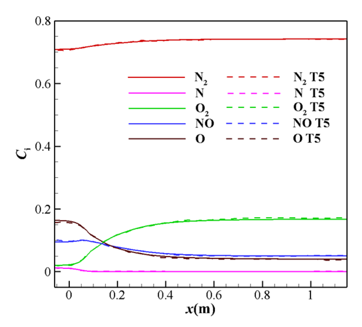
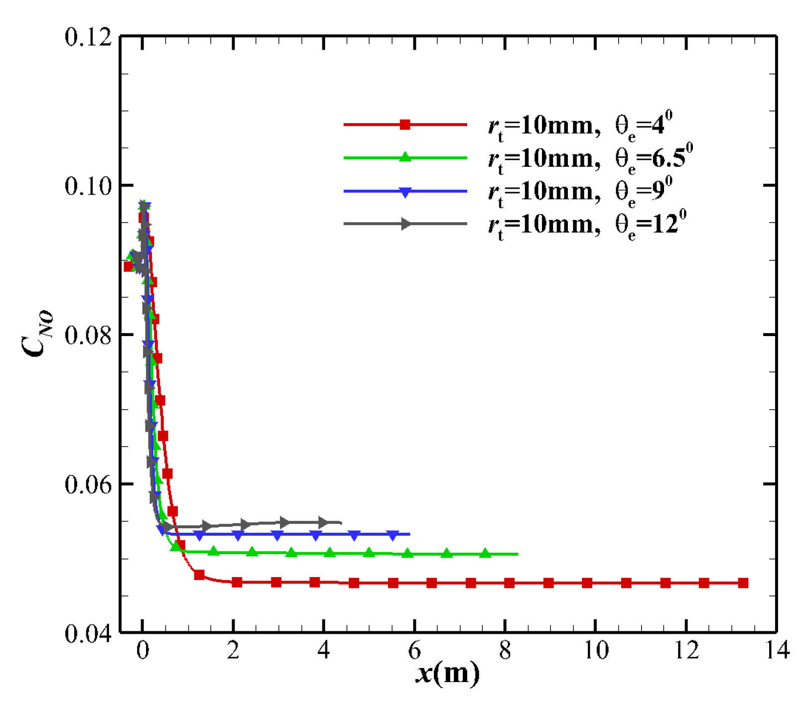
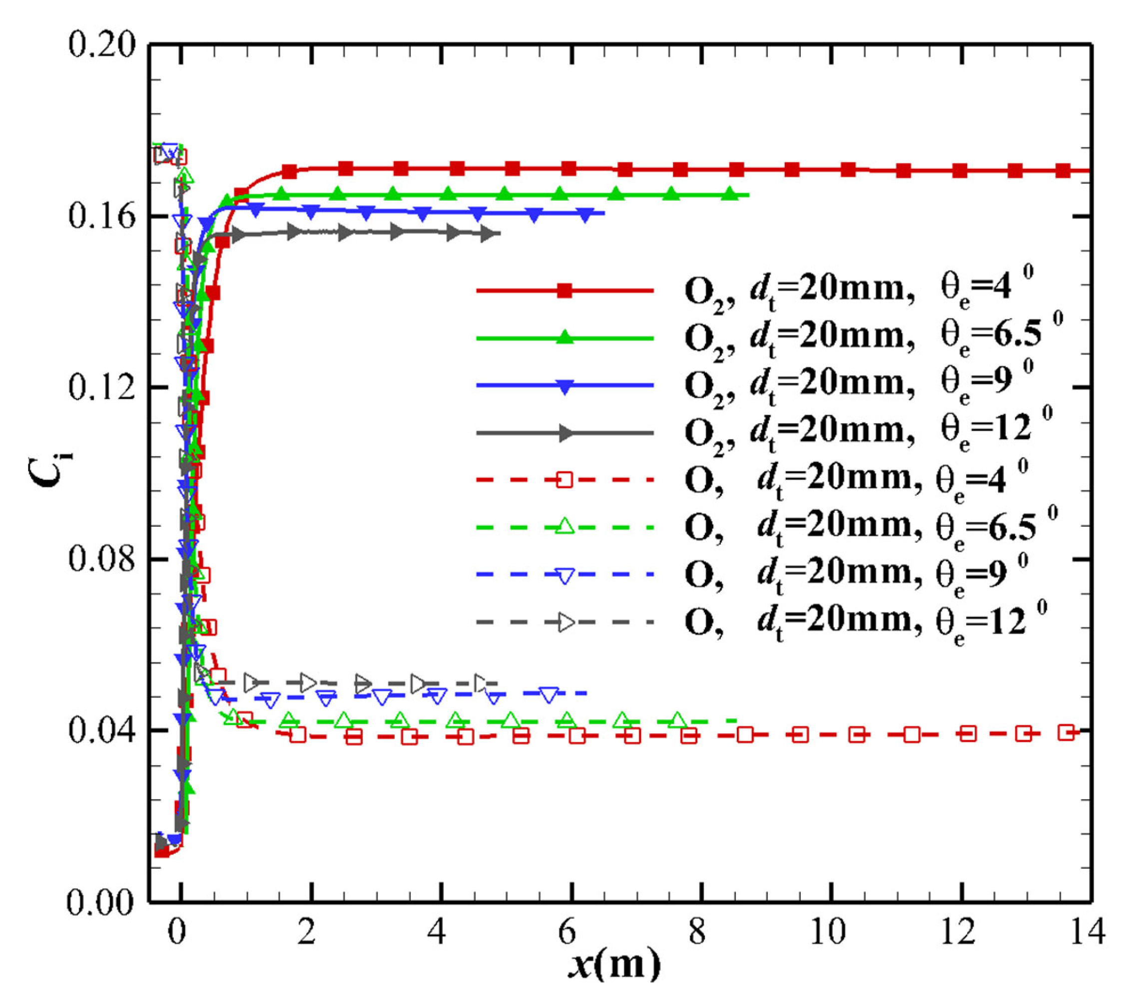
• The thermochemical non-equilibrium expansion effects of the conical nozzle change the species mass fraction, temperature, and Mach number. When the thermochemical nonequilibrium effect is suppressed, more vibrational energy is transmitted to the translational energy, which increases the translational temperature. Under the condition that the exit velocity is basically constant, the Mach number at the nozzle exit decreases. The freezing temperature at the nozzle outlet decreases while the mass fraction of O₂ and N₂ species increase and the mass fraction of other species such as NO, N, and O decrease.

When designing a high enthalpy conical nozzle, it is necessary to consider suppressing the influence of thermochemical nonequilibrium expansion effects so that the nozzle outlet flow field is close to equilibrium flow. Therefore, a smaller maximum expansion angle and a larger nozzle throat can be selected.

References

1. Deutsches Zentrum fur Luft-und Raumfahrt (DLR). The high enthalpy shock tunnel Gottingen of the German Aerospace Center (DLR). J. Large-Scale Res. Facil. 2018, 4, A133. [Google Scholar] [CrossRef]
2. Anderson, J.D. Hypersonic and High Temperature Gas Dynamics, 2nd ed.; AIAA: Orlando, FL, USA, 2006. [Google Scholar]
3. Shang, J.J.S.; Yan, H. High-enthalpy hypersonic flows. Adv. Aerodyn. 2020, 2, 19. [Google Scholar] [CrossRef]
4. Jiang, H.; Liu, J.; Luo, S.; Huang, W.; Wang, J.; Liu, M. Thermochemical non-equilibrium effects on hypersonic shock wave/turbulent boundary-layer interaction. Acta Astronaut. 2022, 192, 1–14. [Google Scholar] [CrossRef]
5. Gu, S.; Olivier, H. Capabilities and limitations of existing hypersonic facilities. Prog. Aerosp. Sci. 2020, 113, 100607. [Google Scholar] [CrossRef]
6. Hannemann, K.; Itoh, K.; Mee, D.J.; Hornung, H.G. Free piston shock tunnels HEG, HIEST, T4 and T5. Exp. Methods Shock. Wave Res. 2016, 9, 181–264. [Google Scholar]
7. Shen, J.; Lu, H.; Li, R.; Chen, X.; Ma, H. The thermochemical non-equilibrium scale effects of the high enthalpy nozzle. Adv. Aerodyn. 2020, 2, 20. [Google Scholar] [CrossRef]
8. Marineau, E.C.; Hornung, H.G. High-enthalpy nonequilibrium nozzle flow: Experiments and computations. In Proceedings of the 39th AIAA Fluid Dynamics Conference and Exhibit, San Antonio, TX, USA, 22–25 June 2009. [Google Scholar]
9. Wilson, Y.K.; Craddock, S.C.; Doherty, L.J. Aerodynamic design of nozzles with uniform outflow for hypervelocity ground-test facilities. J. Propuls. Power 2018, 34, 1467–1478. [Google Scholar]
10. Passiatore, D.; Sciacovelli, L.; Cinnella, P.; Pascazio, G. Thermochemical non-equilibrium effects in turbulent hypersonic boundary layers. J. Fluid Mech. 2022, 941, A21. [Google Scholar] [CrossRef]
11. Clarke, J.; Collen, P.L.; McGilvray, M.; di Mare, L. Numerical simulation of a shock tube in thermochemical non-equilibrium. In Proceedings of the AIAA SCITECH 2023 Forum, National Harbor, MD, USA, 23–27 January 2023. [Google Scholar]
12. Mee, D.J.; Morgan, R.G.; Paull, A.; Jacobs, P.A.; Smart, M.K. The T4 Stalker Tube. In 30th International Symposium on Shock Waves 2: ISSW30-Volume 2; Springer International Publishing: Cham, Switzerland, 2017; pp. 1425–1429. [Google Scholar]
13. Marineau, E.C.; Hornung, H.G. Heat flux Calibration of T5 hypervelocity shock Tunnel conical nozzle in air. In Proceedings of the 47th AIAA Aerospace Sciences Meeting Including The New Horizons Forum and Aerospace Exposition, Orlando, FL, USA, 5–8 January 2009. [Google Scholar]
14. Nagayama, T.; Nagai, H.; Tanno, H.; Komuro, T. Global heat flux measurement using temperature-sensitive paint in high-enthalpy shock tunnel HIEST. In Proceedings of the 55th AIAA Aerospace Sciences Meeting, Grapevine, TX, USA, 9–13 January 2017; p. 1682. [Google Scholar]
15. Hannemann, K. High enthalpy flows in the HEG shock tunnel: Experiment and numerical rebuilding. In Proceedings of the 41st Aerospace Sciences Meeting and Exhibit 2003, Reno, Nevada, 6–9 January 2003. [Google Scholar]
16. Holden, M.S.; Wadhams, T.P.; MacLean, M. Experimental studies in LENS I and X to evaluate real gas effects on hypevelocity vehicle performance. In Proceedings of the 45th AIAA Aerospace Science Meeting and Exhibit, Reno, NV, USA, 8–11 January 2007. [Google Scholar]
17. Matthew, M.; Luke, J.; Doherty, R. Gildfind T6: The Oxford University Stalker Tunnel. In Proceedings of the 20th Aiaa International Space Planes and Hypersonic Systems and Technologies Conference, Glasgow, Scotland, 6–9 July 2015. [Google Scholar]
18. Zhao, W.; Jiang, Z.L.; Saito, T.; Lin, J.M. Performance of a detonation driven shock tunnel. Shock Waves 2005, 14, 53–59. [Google Scholar] [CrossRef]
19. Shen, J.M.; Ma, H.D.; Li, C. Initial measurements of a 2m mach10 free piston shock tunnel at CAAA. In Proceedings of the 31st International Symposium on Shock Waves, Nagoya, Japan, 9–14 July 2017. [Google Scholar]
20. Shen, J.; Dong, J.; Li, R.; Zhang, J.; Chen, X.; Qin, Y.; Ma, H. Integrated supersonic wind tunnel nozzle. Chin. J. Aeronaut. 2019, 32, 2422–2432. [Google Scholar] [CrossRef]
21. Park, C. Assessment of two-temperature kinetic model for ionizing air. J. Thermophys. 1989, 3, 233–252. [Google Scholar] [CrossRef]
22. Campbell, N.S.; Hanquist, K.; Morin, A.; Meyers, J.; Boyd, I. Evaluation of Computational Models for Electron Transpiration Cooling. Aerospace 2021, 8, 243. [Google Scholar] [CrossRef]
23. Rudinskii, A.V.; Yagodnikov, D.A.; Ryzhkov, S.V.; Onufriev, V.V. Features of Intrinsic Electric Field Formation in Low-Temperature Oxygen–Methane Plasma. Tech. Phys. Lett. 2021, 47, 520–523. [Google Scholar] [CrossRef]
24. Maier, W.T.; Needels, J.T.; Garbacz, C.; Morgado, F.; Alonso, J.J.; Fossati, M. SU2-NEMO: An Open-Source Framework for High-Mach Nonequilibrium Multi-Species Flows. Aerospace 2021, 8, 193. [Google Scholar] [CrossRef]
25. Gnoffo, P.A.; Gupta, R.N. Conservation Equations and Physical Models for Hypersonic Air Flows in Thermal and Chemical Nonequilibrium; Report No. TP 2867; NASA: Washington, DC, USA, 1989.
26. Gupta, R.N.; Thompson, R.A. A Review of Reaction Rates and Thermodynamics and Transport Properties for an 11-Species Air Model for Chemical and Thermal Nonequilibrium Calculations to 3000k; Report No. RP-1232; NASA: Washington, DC, USA, 1990.
27. Park, C. Problems of rate chemistry in the flight regimes of aeroassisted orbital transfer vehicles. In Proceedings of the 19th Thermophysics Conference, Snowmass, CO, USA, 25–28 June 1984; Volume 96, pp. 511–537. [Google Scholar]
28. Grant, P.; Michael, J.W. A comparison of methods to compute high temperature gas thermal conductivity. In Proceedings of the 36th AIAA Thermophysics Conference, Orlando, FL, USA, 23–26 June 2003. [Google Scholar]
29. Jameson, A. Solution of the Euler equations for complex configurations. In Proceedings of the 6th Computational Fluid Dynamics Conference, Danvers, MA, USA, 13–15 July 1983. [Google Scholar]
30. Shima, E.; Kitamura, K. On new simple low-dissipation scheme of AUSM-family for all speeds. In Proceedings of the 47th AIAA Aerospace Sciences Meeting Including the New Horizons Forum and Aerospace, Orlando, FL, USA, 5–8 January 2009. [Google Scholar]
31. Candler, G.V. Hypersonic nozzle analysis using an excluded volume equation of state. In Proceedings of the 38th AIAA Thermophysics Conference, Toronto, ON, USA, 6–9 June 2005. [Google Scholar]
32. Wang, Y.; Hu, Z.; Lu, Y. Starting process in a large-scale shock tunnel. AIAA J. 2016, 54, 1240–1249. [Google Scholar] [CrossRef] [Green Version]
33. Spalart, P.R.; Allmaras, S.R. A one-equation turbulence model for aerodynamic flow. In Proceedings of the 30th AIAA Aerospace Science Meeting and Exhibit, Reno, NV, USA, 6–9 January 1992. [Google Scholar]
34. Tyurenkova, V.V.; Stamov, L.I. Flame propagation in weightlessness above the burning surface of material. Acta Astronaut. 2019, 159, 342–348. [Google Scholar] [CrossRef]
35. Zeng, M. Numerical Rebuilding of Free-Stream Measurement and Analysis of Noequilibrium Effects in High Enhtalpy Tunnel. Ph.D. Thesis, Chinese Academy of Sciences, Beijing, China, 2007; pp. 63–64. (In Chinese). [Google Scholar]
36. Smirnov, N.; Betelin, V.; Nikitin, V.; Stamov, L.; Altoukhov, D. Accumulation of errors in numerical simulations of chemically reaction gas dynamics. Acta Astronaut. 2015, 117, 338–355. [Google Scholar] [CrossRef]
37. Smirnov, N.; Betelin, V.; Shagaliev, R.; Nikitin, V.; Belyakov, I.; Deryuguin, Y.; Aksenov, S.; Korchazhkin, D. Hydrogen fuel rocket engines simulation using LOGOS code. Int. J. Hydrog. Energy 2014, 39, 10748–10756. [Google Scholar] [CrossRef]
Figure 1. Computational grid and different domains.
Aerospace 10 00455 g001
Figure 2. Comparison of the centerline species mass fraction distributions.
Aerospace 10 00455 g002
Figure 3. Comparison of centerline temperature distributions based on the different MEAs.
Aerospace 10 00455 g003
Figure 4. Comparison of centerline pressure gradient distribution based on the different MEAs.
Aerospace 10 00455 g004
Figure 5. Comparison of centerline velocity distributions based on the different MEAs.
Aerospace 10 00455 g005
Figure 6. Comparison of centerline temperature distributions based on the different TRs.
Aerospace 10 00455 g006
Figure 7. Comparison of centerline pressure gradient distribution based on the different TRs.
Aerospace 10 00455 g007
Figure 8. Comparison of centerline velocity distributions based on the different TRs.
Aerospace 10 00455 g008
Figure 9. Comparison of centerline temperature distributions based on the different CAs.
Aerospace 10 00455 g009
Figure 10. Comparison of centerline temperature distributions based on the different TCRs.
Aerospace 10 00455 g010
Figure 11. Comparison of centerline Mach number distributions based on the different MEAs.
Aerospace 10 00455 g011
Figure 12. Comparison of centerline speed sound distributions based on the different MEAs.
Aerospace 10 00455 g012
Figure 13. Comparison of the centerline Mach number distributions based on the different TRs.
Aerospace 10 00455 g013
Figure 14. Comparison of centerline NO mass fraction distribution under the different MEAs.
Aerospace 10 00455 g014
Figure 15. Comparison of centerline O2 and O mass fraction distribution for nozzles with different MEAs.
Aerospace 10 00455 g015