An Innovative External Heat Flow Expansion Formula for Efficient Uncertainty Analysis in Spacecraft Earth Radiation Heat Flow Calculations

Abstract

Thermal uncertainty analysis of spacecraft is an important method to avoid overdesign and underdesign problems. In the context of uncertainty analysis, thermal models representing multiple operating conditions must be invoked repeatedly, leading to substantial computational costs. The ray tracing calculation of Earth infrared and albedo radiation heat flux is an important reason for the slow calculation speed. As the rays emitted during external heat flux calculations under different operating conditions are independent and unconnected, the rays produced across various conditions are effectively wasted. In this study, the external heat flow equation is thoroughly expanded and the derived factors are clustered and analyzed to develop a novel formula for calculating external heat flow. When this formula is employed to compute the uncertain external heat flux, only one condition necessitates ray tracing, while the remaining conditions utilize simple matrix operations in place of complex ray tracing. Within the aforementioned procedure, certain matrices demonstrate sparse characteristics. The optimization calculations for these matrices can, therefore, benefit from the application of sparse matrix optimization algorithms. Using a spacecraft as an example, the uncertain external heat flux calculation outcomes of the new and traditional formulas are compared and assessed. The findings reveal that the new formula is highly suitable for estimating uncertain Earth radiation heat flow, with a marked improvement in efficiency. The accuracy is essentially equivalent to that of the traditional formula and the calculation precision can be dynamically adjusted to meet user requirements. The methodology can be further generalized to assess the uncertainties associated with radiative external heat fluxes for other celestial bodies within the solar system. This offers a valuable theoretical framework for addressing the uncertainties in the thermal design of deep space exploration vehicles.

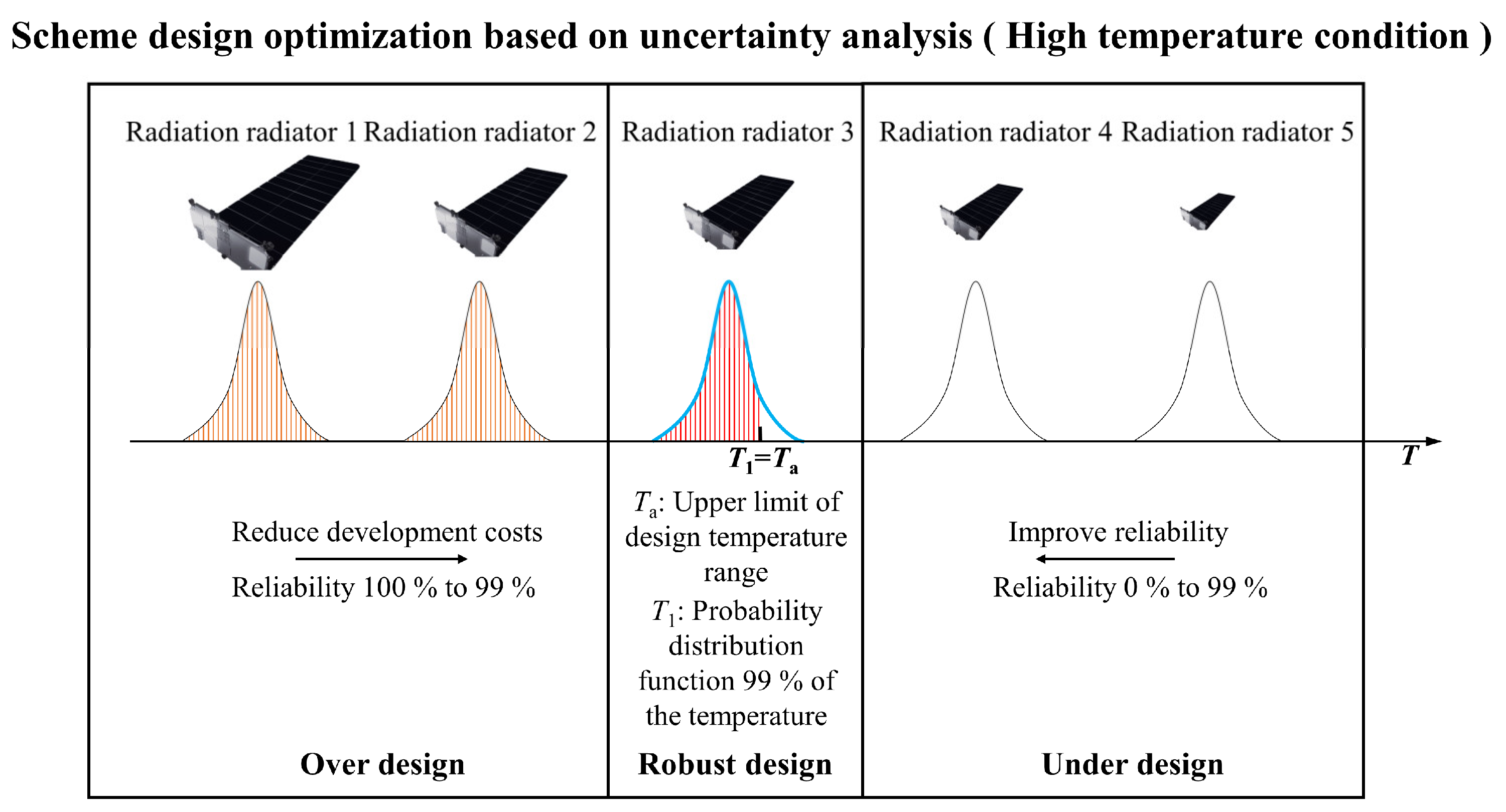
1. Introduction

As aerospace technology advances and application demands continue to expand, the robustness and reliability of spacecraft thermal control systems are subject to increasingly stringent requirements. During the design process of these control systems, assumptions and simplifications made in the spacecraft thermal analysis model can introduce unknown errors into the design analysis outcomes. Furthermore, uncertainties in the performance of structural materials may arise from material defects or machining precision during the manufacturing process, while the external heat flow absorbed by the structure in operation can also vary. The cumulative impact of these uncertainties can influence the temperature field of the spacecraft structure and, under specific circumstances, may even result in equipment damage or failure.

Spacecraft thermal control systems are typically designed and validated based on extreme conditions. The factors considered under these conditions encompass the corresponding worst-case environmental and spacecraft structural parameters. Subsequent analysis reveals that, to address uncertainties stemming from the remaining parameters, a fixed design margin (also referred to as the uncertainty margin) can be applied to the results (downstream of the model). These margins are derived from statistical analyses of the discrepancies between the predicted temperatures of thermal models and the flight measurement outcomes from select space missions [1,2].

Traditional spacecraft thermal design and verification methods do not rigorously address model uncertainty in the upstream portion of the model. Instead, they handle uncertainty downstream by directly applying fixed design margins to the model output. Research conducted by Ishimoto and Bevans (1968) [3], Howell (1973) [4], and Thunnissen (2004) [5] indicate that the primary goal of performing uncertainty analysis is to provide a more effective method for calculating these design margins. The main concept involves strictly considering model uncertainty upstream and propagating it to the output through the model, subsequently quantifying the uncertainty of the model output. Compared with conventional methods, this approach has the advantage of providing design margins under specific circumstances.

As demonstrated in Figure 1, there is a discernible positive correlation between the radiator size, extending from radiator 5 to radiator 1, and its correlated cooling capacity. Notably, an augmentation in size also results in an escalated mass. The practice of mass reduction is a salient objective in spacecraft design, owing to its substantial potential to curtail both the cost and complexity of the mission. Even marginal mass reduction can translate into remarkable savings in terms of fuel and launch costs. Using the selection of a spacecraft radiator model as an example, conducting thermal uncertainty analysis on the radiator can help avoid overdesign scenarios (radiation radiators 1 and 2) that result from excessively large radiation radiator model choices, effectively reducing development costs. Additionally, this analysis can prevent underdesign situations caused by selecting a radiation radiator model that is too small and has insufficient heat dissipation reliability (radiation radiators 4 and 5).

The primary method for spacecraft thermal uncertainty analysis is the Monte Carlo (MC) approach. However, to obtain accurate results, a substantial number of original model simulations are needed, leading to considerable computational costs. This method necessitates numerous spacecraft thermal analyses under various working conditions. If uncertainty analyses were conducted directly based on the spacecraft thermal analysis model, the computational cost would be unacceptably high. Many scholars have conducted research on the balance between the accuracy and efficiency of the thermal uncertainty analysis algorithm. For example, Thunnissen [6] used subset simulation to perform transient thermal uncertainty analysis on the cruise phase of the Mars spacecraft. The tail probability distribution function of the maximum temperature of important components was obtained. The results successfully replicated the MC simulation results and, compared with the MC case, the calculation burden was much lower. Gómez-San-Juan [7] developed a one-dimensional generalized statistical error analysis method. The input uncertainty variables of this method could be arbitrarily distributed and the nonlinear relationship between node temperature and uncertainty variables was incorporated. The calculation time matched that of the statistical error analysis method and the accuracy matched that of the MC approach. Xiong et al. [8] approximated the traditional thermal analysis calculation model of spacecraft based on a radial basis function (RBF) neural network of the improved mind evolutionary algorithm. The trained neural network effectively improved the analysis rate of thermal uncertainty analysis. Kato [9] used a Gaussian process regression simulator and minimum absolute shrinkage selection operator to perform thermal uncertainty analysis on satellites. The simulator reduced the cost of uncertainty quantification. Similar to the above methods, the kriging model [10,11,12,13], RBF method [14], artificial neural network [15,16], support vector regression method [17], and response surface method [18] are all approximate models that replace spacecraft thermal analysis models. Thermal uncertainty analysis can be performed on the approximate model to improve the computational efficiency. However, to obtain an accurate approximation model, the original thermal analysis model of the spacecraft requires repeated calculation.

The existing methods focus on enhancing the computational efficiency of spacecraft thermal uncertainty analysis from a mathematical perspective. In this study, we aim to improve the calculation efficiency of thermal uncertainty analysis by optimizing the original thermal analysis model of spacecraft. During the calculation process of the spacecraft’s original thermal analysis model, there are two main steps to obtain the satellite temperature field: radiation model calculation and thermal model calculation. The radiation model calculation comprises three types of external heat flux absorbed by the spacecraft surface elements and the radiative thermal conductance between these elements. These three types of external heat flow include Earth infrared radiation heat flow, Earth albedo radiation heat flow, and solar radiation heat flow. Thermal model calculations encompass the surface element heat capacity, the linear thermal conductivity between the spacecraft surface elements, the power of the heat source within the surface elements, and the solution of the energy balance equation. Reference [7] highlights that the calculation time of the radiation model is significantly longer than that of the thermal model, with the radiation MC ray tracing calculation being the most time-consuming task. The calculation of external heat flow from Earth infrared and albedo radiation is a crucial aspect of radiation model calculation. In thermal uncertainty analysis, the Monte Carlo ray tracing algorithm needs to be employed multiple times to compute the Earth infrared and albedo radiation heat flux, which is one of the main factors contributing to the immense computational cost of thermal uncertainty analysis.

Owing to the uncertainty of spacecraft thermal property parameters, various thermal property parameter samples are generated in thermal uncertainty analysis. When calculating the external heat flux corresponding to each working condition sample, each solution of the external heat flux is independent. Upon completing the external heat flux calculation for one working condition, the subsequent working condition’s external heat flux calculation does not utilize the rays emitted by the previous working condition. Instead, the new working condition initiates a fresh set of rays and conducts ray tracing. This process leads to the underutilization of rays from the previous working condition, consequently increasing the calculation time.

To address the issue of slow calculation time resulting from underutilized rays, this study thoroughly expands the formulation of Earth infrared and albedo external heat flow, completely isolating the factors of the formulation to develop a new corresponding expression. This formula is employed for uncertain external heat-flow calculations. Only the first condition emits rays, with ray tracing calculations for Earth radiative external heat flow in this condition generating the external heat-flow expansion (EHFE) matrix. For the remaining thermal uncertainty analysis conditions, new thermal attribute parameter samples are substituted into the EHFE matrix. This new formula is highly suitable for the analysis of the uncertain external heat flux, as it eliminates the need to project rays and perform ray tracing for calculating the external heat flux in each condition. Matrix operations are used instead of the original ray tracing calculation process. This approach to calculating the uncertain external heat flux can effectively reduce the calculation time while maintaining sufficient accuracy.

The structure of this paper is organized as follows: Section 2 introduces the solution model for the spacecraft temperature field, the calculation process for Earth radiation external heat flow, and the ray tracing method for external heat-flow calculation. Section 3 presents the current calculation formula for the Earth infrared and albedo radiation heat flux and provides a detailed description of its expansion to provide a new formula. This section also explains how to analyze an uncertain external heat flux using this new formula. In Section 4, a spacecraft is used as an example, with its composition and calculation parameters being introduced. Section 5 discusses and analyzes the results of the spacecraft’s uncertain Earth radiation external heat flow. Finally, conclusions are drawn in Section 6.

2. Thermal Analysis Model of Spacecraft

2.1. Temperature-Field Calculation Model

The order of solving the mathematical thermal model of the spacecraft is as follows. First, radiation calculation is carried out based on a geometric mathematical model. In this process, the MC ray tracing algorithm is used to calculate the radiation heat transfer. Q_S−i, Q_er−i, Q_r−i, and G_ji are calculated and these outputs are input into the mathematical thermal model. The second step is the solution of the mathematical thermal model to obtain the temperature fields of the spacecraft’s surface elements. The expression of the mathematical thermal model is as follows:

$$m_i{c}_i\frac{d{T}_i}{dt}=Q_{\mathrm{S}-i}+Q_{\mathrm{er}-i}+Q_{\mathrm{r}-i}+Q_i+{\displaystyle \sum _{j=1}^N{D}_{ji}}(T_j-T_i)+{\displaystyle \sum _{j=1}^N{G}_{ji}(T_j^4-T_i^4)}$$

(1)

where the subscripts i and j denote surface element (node) numbers; T is temperature; m is mass; c is specific heat; t is time; Q_s−i is the solar heat load on node i; Q_er−i is the planetary albedo heat load on node i; Q_r−i is the planetary infrared heat load on node i; Q is the internal heat source power; D_ji and G_ji denote the linear and radiative thermal conductivity between nodes j and i, respectively [19,20].

Reference [7] highlights that the calculation time required for the radiation model is significantly longer than that of the mathematical thermal model. The MC radiation calculation is the most time-consuming task. In thermal uncertainty analysis, the computation of the external heat flux utilizing the MC ray tracing method demands considerable computational resources; consequently, there is a need for algorithm optimization.

2.2. Earth Radiation Heat Flow Calculation Process

The reverse Monte Carlo (RMC) method is a general approach for computing the Earth infrared and albedo external heat flux absorbed by surface elements. N rays are emitted from the target surface element and ray tracing is conducted on them. The N-ray results are statistically analyzed to determine the Earth infrared and albedo external heat flux for the target surface element. The RMC simulation for a single ray proceeds as follows:

(1)

Reference coordinate systems, such as body, orbit, and geocentric inertial coordinate systems, are established and orbit parameters are provided.

(2)

A thermal–physical model of the spacecraft structure is constructed, the thermal analysis surface element grid is partitioned, and the surface equation and radiation characteristics for each thermal analysis surface element are determined.

(3)

A target surface element of the spacecraft emits a random ray [21].

(4)

The intersection of the ray with the surface element of the system (spacecraft and radiation source) is calculated and the method for further tracking the ray is determined according to the ray tracing technique.

(5)

If the ray is absorbed by the radiation source’s surface, the external heat flux absorbed by the ray on the target surface element’s surface is accounted for using the reverse process.

2.3. Ray Tracing Method for External Heat Flux Calculation

At present, there are three ray tracing methods to calculate the external heat flux [22].

• Collision method: During the ray tracing process, rays are treated as a whole and are not divided into smaller segments. Rays maintain constant energy throughout the tracing process. To calculate the energy absorbed by a surface when a ray strikes it, a random number R_α is selected between 0 and 1 and compared to the surface absorption rate α. If R_α < α, the ray is completely absorbed by the surface and the process ends. If R_α ≥ α, the ray is fully reflected.
• Path length method: In this approach, during ray tracing, a portion of the ray’s energy is absorbed by the surface it impacts, while the remaining energy is reflected and continues to be traced. Calculation of the energy absorbed by the surface does not involve random numbers. A small fraction of the ray’s energy is absorbed by the surface and the rest is reflected. This method functions by preventing the complete termination of a ray in a single collision, allowing each ray to contribute to the results of multiple subregions. This significantly reduces the statistical uncertainty for a given number of rays.
• When analyzing a closed cavity, the rays emitted may result in an infinite loop based on the path length method of propagation. To avoid this, an energy cutoff fraction k (0 < k< 1) is introduced. When the reflected ray energy q₂(1 − α) > kq₁, the path length method is used. When the reflected ray energy q₂(1 − α) ≤ kq₁, ray tracking is halted. q₁ is the energy of the initial surface element emitting the ray. Here, q₂ is the energy of the ray hitting a surface element.

3. Uncertainty Model for the Calculation of Earth Radiative External Heat Flow

3.1. Analysis of Ray Tracing Methods: Uncertainty Issues

The present state of algorithms for uncertainty thermal analysis in spacecraft appears to exhibit a challenge in terms of computational efficiency. Owing to the uncertainty in the solar absorbance and infrared emissivity of spacecraft coatings, conducting thermal uncertainty analysis necessitates invoking the thermal model multiple times and iteratively calculating the external heat flow. It generates huge computational costs. Employing traditional methods for external heat flow calculation requires re-emitting rays each time, resulting in the issue of wasted rays. This study presents a detailed analysis of ray tracing, in which every emitted ray is fully utilized during the thermal uncertainty analysis. When the surface properties of the spacecraft coating are altered, rays emitted by the previous model are employed, thus eliminating the need to re-emit rays for calculating the Earth radiated external heat flow under the given condition.

In this investigation, the Earth radiative external heat flow calculation equation is fully expanded. By substituting the intricate process of ray tracing with rudimentary matrix operations, there is a substantive reduction in computational expenditures. This allows for accurate and expedited uncertainty thermal analysis. This methodology aids in the development of more proficient and dependable thermal control systems; it also enhances the performance of onboard instrumentation and systems. Moreover, it facilitates extended mission durations, bolsters safety, and promotes cost efficiency.

3.1.1. Earth Infrared Radiation External Heat Flow: Collision Method

This paper is based on the energy conservation relationship of the Earth infrared radiation and the basic principle of the RMC method emission of rays from the spacecraft target surface element and ray tracing using the collision method. N_ei beams of rays emitted from the surface element E_i are tracked, with N_ai beams reaching the Earth surface and being absorbed. Then, the density of the external heat flow from the Earth infrared radiation absorbed by the surface element E_i can be expressed as:

$$q_{\mathrm{r}}^i=\frac{1}{N_{\mathrm{ei}}}(N_{\mathrm{ai}}\times \frac{1-\mathsf{\rho }}{4}\times \mathrm{S}\times {\epsilon }_{{\mathrm{E}}_i}^{\mathrm{r}})$$

(2)

where ρ is the Earth average solar albedo with a value of 0.35; S is the solar constant with a value of 1353 W/m²; ${\epsilon }_{{\mathrm{E}}_i}^r$ is the infrared emissivity of the surface element E_i coating [23,24,25,26,27,28].

3.1.2. Earth Infrared Radiation External Heat Flow: Pathlength Method and Cutoff Factor

Rays are emitted from the spacecraft target surface element and ray tracing is performed using the latter two methods. N_r beams of rays emitted from the spacecraft’s surface element E_i are tracked, with $N_{\mathrm{r}}^{\mathrm{A}}$ rays reaching the Earth surface directly. Then, the density of the external heat flow from the Earth infrared direct radiation absorbed by the surface element E_i can be expressed as:

$$q_{\mathrm{r},\mathrm{A}}^i=\frac{1}{N_{\mathrm{r}}}(N_{\mathrm{r}}^{\mathrm{A}}\times \frac{1-\mathsf{\rho }}{4}\times \mathrm{S}\times {\alpha }_{E_i}^{\mathrm{r}})$$

(3)

where $q_{\mathrm{r},\mathrm{A}}^i$ denotes the density of the Earth infrared direct radiation heat flow to the surface element E_i; ${\alpha }_{{\mathrm{E}}_i}^{\mathrm{r}}$, the infrared absorbance of the spacecraft surface element E_i, is equal to the coating infrared emissivity [23,24,25,26,27,28].

N_r beams of rays emitted from the spacecraft’s surface element E_i are tracked, with $N_{\mathrm{r}}^{\mathrm{B}}$ beams reaching the Earth surface after multiple reflections. Then, the external heat flow from the Earth infrared indirect radiation absorbed by the surface element E_i can be expressed as:

$$q_{\mathrm{r},\mathrm{B}}^i=\frac{1}{N_{\mathrm{r}}}({\displaystyle \sum _{j=1}^{N_{\mathrm{r}}^{\mathrm{B}}}\frac{1-\mathsf{\rho }}{4}}\times \mathrm{S}\times {\alpha }_{{\mathrm{E}}_i}^{\mathrm{r}}\times K_{\mathrm{r}}^j)$$

(4)

where $K_{\mathrm{r}}^j={\displaystyle \prod _{\tau =1}^k(1-{\alpha }_{{\mathrm{E}}_{\tau }}^{\mathrm{r}}})$, with k being the number of reflections [23,24,25,26,27,28].

In summary, the total external heat flow density of the Earth infrared radiation absorbed by the surface element E_i is

$$q_{\mathrm{r}}^i=q_{\mathrm{r},\mathrm{A}}^i+q_{\mathrm{r},\mathrm{B}}^i$$

(5)

3.1.3. Earth Albedo Radiation External Heat Flow: Collision Method

This paper is based on the energy conservation relationship of Earth albedo radiation and the basic principles of the RMC method. By emitting rays from the spacecraft target surface element and using the collision method for ray tracing, N_ei beams of rays emanating from surface element E_i are tracked, with N_ai rays reaching the Earth surface and being absorbed. The angle θ_se between the outer normal vector of the ray’s intersection with the Earth and the direction vector of the sun rays is greater than 90°. Then, the density of the external heat flow from the Earth albedo radiation absorbed by surface element E_i can be expressed as:

$$q_{\mathrm{er}}^i=\frac{1}{N_{\mathrm{ei}}}({\displaystyle \sum _{j=1}^{N_{\mathrm{ai}}}\mathsf{\rho }}\times \mathrm{S}\times {\alpha }_{{\mathrm{E}}_i}^{\mathrm{er}}\times \left|\cos {\theta }_{\mathrm{se}}^j\right|)$$

(6)

where ${\alpha }_{{\mathrm{E}}_i}^{\mathrm{er}}$ is the solar absorptance of the surface element E_i coating [23,24,25,26,27,28].

3.1.4. Earth Albedo Radiation External Heat Flow: Path Length Method and Cutoff Factor

Rays are emitted from the target surface element of the spacecraft and ray tracing is performed using the latter two methods. N_er beams of rays from the spacecraft’s surface element E_i are tracked, with $N_{\mathrm{er}}^{\mathrm{A}}$ beams reaching the Earth’s surface directly. The angle θ_se between the outer normal vector of the intersection of the ray and the Earth and the direction vector of the sun’s rays is greater than 90°. Then, the external heat flow from the Earth albedo direct radiation absorbed by the surface element E_i can be expressed as:

$$q_{\mathrm{er},\mathrm{A}}^i=\frac{1}{N_{\mathrm{er}}}({\displaystyle \sum _{j=1}^{N_{\mathrm{er}}^{\mathrm{A}}}\mathsf{\rho }}\times \mathrm{S}\times {\alpha }_{{\mathrm{E}}_i}^{\mathrm{er}}\times \left|\cos {\theta }_{\mathrm{se}}^j\right|)$$

(7)

where $q_{\mathrm{er},\mathrm{A}}^i$ denotes the density of direct Earth albedo radiation heat flow to the surface element E_i; ${\alpha }_{{\mathrm{E}}_i}^{\mathrm{er}}$ is the solar absorptance of spacecraft surface element E_i; θ_se is the angle between the direction vector of the sun’s rays and the outer normal vector of rays emitted by surface element E_i hitting the Earth surface intersection [23,24,25,26,27,28].

N_er beams of rays emitted from surface element E_i are tracked and $N_{\mathrm{er}}^{\mathrm{B}}$ beams are reflected several times to reach the Earth surface. The angle θ_se between the outer normal vector of the intersection of the ray and the Earth and the direction vector of the sun’s rays is greater than 90°. Then, the external heat flow from the Earth albedo indirect radiation absorbed by the surface element E_i can be expressed as:

$$q_{\mathrm{er},\mathrm{B}}^i=\frac{1}{N_{\mathrm{er}}}({\displaystyle \sum _{j=1}^{N_{\mathrm{er}}^{\mathrm{B}}}\mathsf{\rho }}\times \mathrm{S}\times {\alpha }_{{\mathrm{E}}_i}^{\mathrm{e}r}\times K_{\mathrm{er}}^j\times \left|\cos {\theta }_{\mathrm{se}}^j\right|)$$

(8)

where $K_{\mathrm{er}}^j={\displaystyle \prod _{\tau =1}^k(1-{\alpha }_{{\mathrm{E}}_{\tau }}^{\mathrm{er}}})$, with k being the number of reflections [23,24,25,26,27,28].

In summary, the total external heat flow density of the Earth albedo radiation absorbed by surface element E_i is:

$$q_{\mathrm{er}}^i=q_{\mathrm{er},\mathrm{A}}^i+q_{\mathrm{er},\mathrm{B}}^i$$

(9)

3.1.5. Comparative Analysis of Calculation Formulas for Various Methods

The collision method is employed to compute the Earth radiative external heat flow. Random numbers must be generated and compared with the absorption rate corresponding to the impacted surface element to determine whether the rays are absorbed or reflected. In the external heat flow calculation equations (Equations (2) and (6)), only the absorption rate of the target surface element is available; information on the coating of the surface element struck during ray propagation is absent. For this type of ray tracing, separating absorbance and reflectance from the equation is unfeasible. If the surface properties of the spacecraft coating change, rays emitted by the previous working model cannot be utilized.

In contrast, the second and third ray tracing methods provide information on the coatings impacting surface elements during ray propagation, as found in Equations (4) and (8) of the Earth radiative external heat flow calculation. These two methods enable the separation of absorptivity and reflectance from the equation. There is no need to re-emit rays when the surface properties of the spacecraft coating change, as the separated expansion formula can be used for direct calculations.

3.2. Earth Radiative EHFE Algorithm

The Monte Carlo method is employed to generate N_S working conditions for the thermal uncertainty analysis of the spacecraft. Radiative model calculations are significantly more time-consuming than thermal model calculations, primarily due to multiple instances of ray tracing and the utilization of the intersection evaluation algorithm. Uncertainty analysis necessitates multiple applications of the external heat flow calculation model, as well as numerous ray tracing and intersection evaluations. In each of these N_S conditions, emitted rays are independent, with no interconnection between them. Consequently, rays from the previous working condition are not utilized in the subsequent working condition. This arises from the incomplete separation of individual variables within the external heat flow solution equation. For the Earth radiative external heat flow solution, the uncertainty variables predominantly involve the infrared emissivity and solar absorbance of the spacecraft surface coating.

As analyzed in Section 3.1, employing the latter two ray tracing methods allows the aforementioned uncertainty variables to be separated. Therefore, this paper adopts the path length method with the introduction of a cutoff factor, where the cutoff factor is set to 0.1. The external heat flow equation is fully expanded to isolate the uncertainty variables within the equation, constituting a new formula for calculating the Earth radiative external heat flow. This approach facilitates an uncertainty analysis of the external heat flow absorbed by the spacecraft.

3.2.1. Earth Infrared Radiation EHFE Equation

A ray originating from an initial surface element that directly reaches Earth is classified as a component of Earth infrared direct radiation external heat flow. Such rays are depicted in Figure 2a. Conversely, if a ray undergoes multiple reflections on the spacecraft’s surface prior to ultimately arriving at Earth, it is regarded as a constituent of Earth infrared radiation indirect external heat flow. Corresponding rays are demonstrated in Figure 2b–d. To fully separate the coating’s infrared emissivity and the corresponding infrared spectrum’s reflectance from the equation, the Earth infrared radiated external heat flow is further expanded, as demonstrated in Equation (10).

The second term indicates that the rays are reflected once on the spacecraft’s surface before reaching Earth, representing a single reflection of Earth infrared radiation external heat flow, as shown in Figure 2b. The third term signifies that the rays are reflected twice on the spacecraft’s surface before reaching Earth, corresponding to a secondary reflection of Earth infrared radiation external heat flow, as depicted in Figure 2c. The nth term implies that the rays are reflected n − 1 time on the spacecraft’s surface before reaching Earth, representing the n − 1th reflection of Earth infrared radiation external heat flow.

$$q_{\mathrm{r}}^i=\frac{1}{N_{\mathrm{r}}}\left\{\begin{array}{l}{N}_{\mathrm{r}}^{{\mathrm{A}}_0}(\frac{1-\mathsf{\rho }}{4}\ast \mathrm{S}\ast {\alpha }_{{\mathrm{E}}_i}^{\mathrm{r}})+{\displaystyle \sum _{j_1=1}^{N_{\mathrm{r}}^{{\mathrm{A}}_1}}(\frac{1-\mathsf{\rho }}{4}\ast \mathrm{S}\ast {\alpha }_{{\mathrm{E}}_i}^{\mathrm{r}})\ast K_1^{{\mathrm{r}}_{j_1}}+}\\ {\displaystyle \sum _{j_2=1}^{N_{\mathrm{r}}^{{\mathrm{A}}_2}}(\frac{1-\mathsf{\rho }}{4}\ast \mathrm{S}\ast {\alpha }_{{\mathrm{E}}_i}^{\mathrm{r}})\ast K_2^{{\mathrm{r}}_{j_2}}}+\cdot \cdot \cdot +{\displaystyle \sum _{j_{n-1}=1}^{N_{\mathrm{r}}^{{\mathrm{A}}_{n-1}}}(\frac{1-\mathsf{\rho }}{4}\ast \mathrm{S}\ast {\alpha }_{{\mathrm{E}}_i}^{\mathrm{r}})\ast K_{n-1}^{{\mathrm{r}}_{j_{n-1}}}}\end{array}\right\}$$

(10)

where $K_1^{{\mathrm{r}}_{j_1}}={\mathsf{\rho }}_{{\mathrm{E}}_{1,1}}^{{\mathrm{r}}_{j_1}}$, $K_2^{{\mathrm{r}}_{j_2}}={\mathsf{\rho }}_{{\mathrm{E}}_{1,2}}^{{\mathrm{r}}_{j_2}}\times {\mathsf{\rho }}_{{\mathrm{E}}_{2,2}}^{{\mathrm{r}}_{j_2}}$, …, $K_{n-1}^{{\mathrm{r}}_{j_{n-1}}}={\displaystyle \prod _{\tau =1}^{n-1}{\mathsf{\rho }}_{{\mathrm{E}}_{\tau ,n-1}}^{{\mathrm{r}}_{j_{n-1}}}}$ and where ${\mathsf{\rho }}_{{\mathrm{E}}_{\tau ,n-1}}^{{\mathrm{r}}_{j_{n-1}}}$ is the infrared spectrum reflectance of the τth intersection of the j_n−1th ray in the nth term of the corresponding EHFE for the surface element coating.

According to Equation (10), surface element E_i emits a total of N_r rays. $N_{\mathrm{r}}^{{\mathrm{A}}_0}$ of them reach the Earth directly, $N_{\mathrm{r}}^{{\mathrm{A}}_1}$ rays reach the Earth after one reflection, $N_{\mathrm{r}}^{{\mathrm{A}}_2}$ rays reach the Earth after two reflections, and $N_{\mathrm{r}}^{{\mathrm{A}}_{n-1}}$ rays reach the Earth after n−1 reflection. $N_{\mathrm{r}}^{{\mathrm{A}}_0}$, $N_{\mathrm{r}}^{{\mathrm{A}}_1}$, $N_{\mathrm{r}}^{{\mathrm{A}}_2}$, …, $N_{\mathrm{r}}^{{\mathrm{A}}_{n-1}}$ satisfy Equation (11).

$$N_{\mathrm{r}}^{{\mathrm{A}}_0}+N_{\mathrm{r}}^{{\mathrm{A}}_1}+N_{\mathrm{r}}^{{\mathrm{A}}_2}+\cdot \cdot \cdot +N_{\mathrm{r}}^{{\mathrm{A}}_{n-1}}\le N_{\mathrm{r}}$$

(11)

The Earth infrared radiation EHFE in Equation (10) is split into a matrix multiplicative form. The applicable formula is $q_{\mathrm{r}-\mathrm{old}}^i=\frac{1}{N_{\mathrm{r}}}\times C_{\mathrm{r}}\times D_{\mathrm{r}}$. Assuming n = 3 in the equation, the Earth infrared radiation external heat flow consists of the Earth infrared direct radiation external heat flow, the primary reflective Earth infrared radiation external heat flow, and the secondary reflective Earth infrared radiation external heat flow.

For the EHFE equation, the D_r matrix is the infrared spectral reflectance combination matrix.

$$D_{\mathrm{r}}={\left[\begin{array}{c}{A}_{\mathrm{r}}(1,1)\times A_{\mathrm{r}}(1,2)\times A_{\mathrm{r}}(1,3)\\ A_{\mathrm{r}}(2,1)\times A_{\mathrm{r}}(2,2)\times A_{\mathrm{r}}(2,3)\\ ⋮\\ A_{\mathrm{r}}(n_{\mathrm{r}}^{\mathrm{m}},1)\times A_{\mathrm{r}}(n_{\mathrm{r}}^{\mathrm{m}},2)\times A_{\mathrm{r}}(n_{\mathrm{r}}^{\mathrm{m}},3)\end{array}\right]}_{n_{\mathrm{r}}^{\mathrm{m}}\times 1}$$

(12)

The element composition of the A_r matrix is shown in Equation (14).

The C_r matrix corresponds to each common factor of the EHFE formula. One of the uncertainty parameters is the infrared emissivity ${\alpha }_{{\mathrm{E}}_i}^{\mathrm{r}}$ of the surface element E_i coating.

$$C_{\mathrm{r}}={\left[\begin{array}{ccc}\frac{1-\mathsf{\rho }}{4}\times \mathrm{S}\times {\alpha }_{{\mathrm{E}}_i}^{\mathrm{r}}& \cdots & \frac{1-\mathsf{\rho }}{4}\times \mathrm{S}\times {\alpha }_{{\mathrm{E}}_i}^{\mathrm{r}}\end{array}\right]}_{1\times n_{\mathrm{r}}^{\mathrm{m}}}$$

(13)

where $n_{\mathrm{r}}^{\mathrm{m}}=N_{\mathrm{r}}^{{\mathrm{A}}_0}+N_{\mathrm{r}}^{{\mathrm{A}}_1}+\cdots +N_{\mathrm{r}}^{{\mathrm{A}}_{n-1}}$. When n = 3, $n_{\mathrm{r}}^{\mathrm{m}}=N_{\mathrm{r}}^{{\mathrm{A}}_0}+N_{\mathrm{r}}^{{\mathrm{A}}_1}+N_{\mathrm{r}}^{{\mathrm{A}}_2}$.

$$A_{\mathrm{r}}={\left[\begin{array}{ccc}1& 1& 1\\ ⋮& ⋮& ⋮\\ {\mathsf{\rho }}_{{\mathrm{E}}_{1,1}}^{{\mathrm{r}}_1}& 1& 1\\ ⋮& ⋮& ⋮\\ {\mathsf{\rho }}_{{\mathrm{E}}_{1,1}}^{{\mathrm{r}}_{N_{\mathrm{r}}^{{\mathrm{A}}_1}}}& 1& 1\\ ⋮& ⋮& ⋮\\ {\mathsf{\rho }}_{{\mathrm{E}}_{1,2}}^{{\mathrm{r}}_1}& {\mathsf{\rho }}_{{\mathrm{E}}_{2,2}}^{{\mathrm{r}}_1}& 1\\ ⋮& ⋮& ⋮\\ {\mathsf{\rho }}_{{\mathrm{E}}_{1,2}}^{{\mathrm{r}}_{N_{\mathrm{r}}^{{\mathrm{A}}_2}}}& {\mathsf{\rho }}_{{\mathrm{E}}_{2,2}}^{{\mathrm{r}}_{N_{\mathrm{r}}^{{\mathrm{A}}_2}}}& 1\end{array}\right]}_{{}_{(N_{\mathrm{r}}^{{\mathrm{A}}_0}+N_{\mathrm{r}}^{{\mathrm{A}}_1}+N_{\mathrm{r}}^{{\mathrm{A}}_2})\times 3}}$$

(14)

The A_r matrix consists of the infrared spectral reflectance of the surface elements. As described below, the first $N_{\mathrm{r}}^{{\mathrm{A}}_0}$ rows of the A_r matrix correspond to the expansion coefficients of the first term of the EHFE equation for the Earth infrared direct radiation external heat flow. As the rays strike the Earth directly, all elements are 1. Rows $N_{\mathrm{r}}^{{\mathrm{A}}_0}+1$ to $N_{\mathrm{r}}^{{\mathrm{A}}_0}+N_{\mathrm{r}}^{{\mathrm{A}}_1}$ correspond to the expansion factor $K_1^{{\mathrm{r}}_{j_1}}$ of the second term of the EHFE equation. The elements in the first column represent the reflectance of the infrared spectrum for the surface element where the rays intersect for the first time; the second and third columns are 1. Rows $N_{\mathrm{r}}^{{\mathrm{A}}_0}+N_{\mathrm{r}}^{{\mathrm{A}}_1}+1$ to $N_{\mathrm{r}}^{{\mathrm{A}}_0}+N_{\mathrm{r}}^{{\mathrm{A}}_1}+N_{\mathrm{r}}^{{\mathrm{A}}_2}$ correspond to the expansion factor $K_2^{{\mathrm{r}}_{j_2}}$ of the third term of the EHFE equation. The elements in the first column represent the reflectance of the infrared spectrum for the surface element where the rays intersect for the first time. The elements in the second column represent the reflectances of the infrared spectrum of the surface element where the rays intersect for the second time. The elements in the third column are 1.

$$H_{\mathrm{r}}={\left[\begin{array}{ccc}0& 0& 0\\ ⋮& ⋮& ⋮\\ {\alpha }_{{\mathrm{E}}_{1,1}}^{{\mathrm{r}}_1}& 0& 0\\ ⋮& ⋮& ⋮\\ {\alpha }_{{\mathrm{E}}_{1,1}}^{{\mathrm{r}}_{N_{\mathrm{r}}^{{\mathrm{A}}_1}}}& 0& 0\\ {\alpha }_{{\mathrm{E}}_{1,2}}^{{\mathrm{r}}_1}& {\alpha }_{{\mathrm{E}}_{2,2}}^{{\mathrm{r}}_1}& 0\\ ⋮& ⋮& ⋮\\ {\alpha }_{{\mathrm{E}}_{1,2}}^{{\mathrm{r}}_{N_{\mathrm{r}}^{{\mathrm{A}}_2}}}& {\alpha }_{{\mathrm{E}}_{2,2}}^{{\mathrm{r}}_{N_{\mathrm{r}}^{{\mathrm{A}}_2}}}& 0\end{array}\right]}_{{}_{(N_{\mathrm{r}}^{{\mathrm{A}}_0}+N_{\mathrm{r}}^{{\mathrm{A}}_1}+N_{\mathrm{r}}^{{\mathrm{A}}_2})\times 3}}$$

(15)

According to the relationship α + ρ = 1, the elements of the A_r matrix are derived from the H_r matrix, where the elements of the H_r matrix represent the corresponding surface element infrared emissivities.

Prior to conducting the uncertainty analysis, the Earth infrared radiation external heat flow absorbed by the primary target surface element must be determined using the RMC method. The number of intersecting face elements and the corresponding infrared emissivities for each ray are recorded and summarized in the intersecting face element number matrix I_r and matrix H_r, respectively. Subsequently, uncertainty analysis of Earth infrared radiation external heat flow is performed for each operating condition without employing ray tracing, as in the traditional method. Instead, a sample of coated infrared emissivities is generated using random numbers. The C_r matrix is then updated to create the C_r¹ matrix and the H_r matrix is updated to form the H_r¹ matrix based on the I_r matrix. The A_r¹ matrix is calculated using the H_r¹ matrix, which is subsequently utilized to compute the D_r¹ matrix. Finally, by substituting the resulting matrices into Equation (17), the Earth infrared radiation external heat flow, accounting for uncertainties, can be obtained.

In this paper, it is crucial to note that the elements constituting the rows of matrices I_r, H_r, A_r, and D_r can be permuted in any desired sequence. The current study organizes the elements within each row of the matrices in a specific manner to facilitate concise and clear communication. During the actual computational process, the elements in each row of I_r, H_r, A_r, and D_r are generated directly based on the sequence of rays emitted by the surface elements.

$$D_{\mathrm{r}}^1={\left[\begin{array}{c}{A}_{\mathrm{r}}^1(1,1)\times A_{\mathrm{r}}^1(1,2)\times A_{\mathrm{r}}^1(1,3)\\ A_{\mathrm{r}}^1(2,1)\times A_{\mathrm{r}}^1(2,2)\times A_{\mathrm{r}}^1(2,3)\\ ⋮\\ A_{\mathrm{r}}^1(n_{\mathrm{r}}^{\mathrm{m}},1)\times A_{\mathrm{r}}^1(n_{\mathrm{r}}^{\mathrm{m}},2)\times A_{\mathrm{r}}^1(n_{\mathrm{r}}^{\mathrm{m}},3)\end{array}\right]}_{n_{\mathrm{r}}^{\mathrm{m}}\times 1}$$

(16)

The equation for the Earth infrared radiation external heat flow taking into account uncertainties is as follows:

$$q_{\mathrm{r}-\mathrm{new}}^i=\frac{1}{N_{\mathrm{r}}}\times C_{\mathrm{r}}^1\times D_{\mathrm{r}}^1$$

(17)

The comparison of two processes for calculating the Earth infrared radiation external heat flow considering parameter uncertainties is in Figure 3.

The main steps of the conventional method for solving the Earth infrared radiative external heat flow considering uncertainties are as follows:

(1)

Samples of all surface element infrared emissivity and corresponding infrared spectral reflectance of the spacecraft are generated using random numbers.

(2)

The RMC method is used to perform ray tracing to solve for the Earth infrared radiation external heat flow.

(3)

The first two steps are repeated to generate multiple $q_{\mathrm{r}}^i$ samples for statistical analysis.

The main steps in solving the Earth infrared radiation external heat flow considering uncertainties using the EHFE formula are as follows:

(1)

The RMC method incorporating ray tracing is used to solve the Earth infrared radiation external heat flow and to obtain the I_r matrix and H_r matrix.

(2)

Samples of all surface element infrared emissivity and corresponding infrared spectral reflectance of the spacecraft are generated using random numbers.

(3)

Based on the new infrared emissivity sample and the intersecting surface element numbering matrix I_r, the corresponding elements of matrices A_r, H_r, and C_r are updated. Matrices A_r¹, H_r¹, and C_r¹ that take into account the uncertainty parameters are generated. Matrix A_r¹ is used to obtain matrix D_r¹.

(4)

Equation (17) allows solution for $q_{\mathrm{r}-\mathrm{new}}^i$.

(5)

Steps (2)–(4) are repeated to generate multiple $q_{\mathrm{r}-\mathrm{new}}^i$ samples to be used for statistical analysis.

In summary, the equation for solving the original Earth infrared radiative external heat flow is expanded. The clustering analysis of each item of the equation constructs a new solution equation $q_{\mathrm{r}-\mathrm{old}}^i=\frac{1}{N_{\mathrm{r}}}\times C_{\mathrm{r}}\times D_{\mathrm{r}}$ for the Earth infrared radiation external heat flow. Thermal uncertainty analysis based on this formula is ray traced for only one operating condition and no rays need to be emitted for other conditions. For other working condition calculations, the new infrared emissivity and infrared spectral reflectance samples are substituted into the position of the corresponding matrix of $q_{\mathrm{r}-\mathrm{new}}^i=\frac{1}{N_{\mathrm{r}}}\times C_{\mathrm{r}}^1\times D_{\mathrm{r}}^1$ and matrix operations are performed. Utilizing matrix operations instead of the original ray tracing approach can effectively reduce the computational cost associated with thermal uncertainty analysis.

3.2.2. Earth Albedo Radiation EHFE Equation

A ray originating from the initial surface element that directly strikes the Earth is considered. The angle θ_se between the outer normal vector of its intersection with the Earth and the direction vector of the sun’s rays is greater than 90°. In this case, the ray constitutes a component of the Earth albedo direct radiation external heat flow. This type of ray is illustrated in Figure 2a. If the ray is reflected multiple times on the spacecraft’s surface before reaching the Earth and the angle θ_se between the outer normal vector of its intersection with the Earth and the direction vector of the sun’s rays remains greater than 90°, then the ray is considered part of the Earth albedo indirect radiation external heat flow. Such rays are depicted in Figure 2b–d. To accurately isolate the coating solar absorptance, the Earth albedo radiation external heat flow is further expanded as in Equation (18). The second term of this equation signifies that the ray impacts the Earth’s surface after a single reflection on the spacecraft’s surface, corresponding to the one-time reflection of the Earth albedo radiation external heat flow, with such rays displayed in Figure 2b. The third term indicates that the ray reaches the Earth’s surface after two reflections on the spacecraft’s surface, representing a two-time reflection of the Earth albedo radiation external heat flow, with rays of this type shown in Figure 2c. The nth term suggests that the ray collides with the Earth’s surface after n − 1 reflections on the spacecraft’s surface, which corresponds to the n−1th reflection of the Earth albedo radiation external heat flow.

$$q_{\mathrm{er}}^i=\frac{1}{N_{\mathrm{er}}}\left\{\begin{array}{cc}\hfill & \sum _{j_0=1}^{N_{\mathrm{er}}^{{\mathrm{A}}_0}}\mathsf{\rho }\times \mathrm{S}\times {\alpha }_{{\mathrm{E}}_i}^{\mathrm{er}}\times \left|cos{\theta }_{\mathrm{se},0}^{j_0}\right|+\sum _{j_1=1}^{N_{\mathrm{er}}^{{\mathrm{A}}_1}}\mathsf{\rho }\times \mathrm{S}\times {\alpha }_{{\mathrm{E}}_i}^{\mathrm{er}}\times \left|cos{\theta }_{\mathrm{se},1}^{j_1}\right|\times K_1^{\mathrm{e}{\mathrm{r}}_{j_1}}+\hfill \\ \hfill & \sum _{j_2=1}^{N_{\mathrm{er}}^{{\mathrm{A}}_2}}\mathsf{\rho }\times \mathrm{S}\times {\alpha }_{{\mathrm{E}}_i}^{\mathrm{er}}\times \left|cos{\theta }_{\mathrm{se},2}^{j_2}\right|\times K_2^{\mathrm{e}{\mathrm{r}}_{j_2}}+\cdots +\sum _{j_{n-1}=1}^{N_{\mathrm{er}}^{{\mathrm{A}}_{n-1}}}\mathsf{\rho }\times \mathrm{S}\times {\alpha }_{{\mathrm{E}}_i}^{\mathrm{er}}\times \left|cos{\theta }_{\mathrm{se},n-1}^{j_{n-1}}\right|\times K_{n-1}^{\mathrm{e}{\mathrm{r}}_{j_{n-1}}}\hfill \end{array}\right\}$$

(18)

where $K_1^{{\mathrm{er}}_{j_1}}={\mathsf{\rho }}_{{\mathrm{E}}_{1,1}}^{{\mathrm{er}}_{j_1}}$, $K_2^{{\mathrm{er}}_{j_2}}={\mathsf{\rho }}_{{\mathrm{E}}_{1,2}}^{{\mathrm{er}}_{j_2}}\times {\mathsf{\rho }}_{{\mathrm{E}}_{2,2}}^{{\mathrm{er}}_{j_2}}$, …, $K_{n-1}^{{\mathrm{er}}_{j_{n-1}}}={\displaystyle \prod _{\tau =1}^{n-1}{\mathsf{\rho }}_{{\mathrm{E}}_{\tau ,n-1}}^{{\mathrm{er}}_{j_{n-1}}}}$, with ${\mathsf{\rho }}_{{\mathrm{E}}_{\tau ,n-1}}^{{\mathrm{er}}_{j_{n-1}}}$ being the reflectance of the solar spectrum for the face element of the τth intersection of the j_n−1th ray in the nth term of the corresponding expansion.

According to Equation (18), the surface element E_i emits a total of N_er rays, $N_{\mathrm{er}}^{{\mathrm{A}}_0}$ of which strike the Earth directly. There are $N_{\mathrm{er}}^{{\mathrm{A}}_1}$ rays that strike the Earth after one reflection. There are $N_{\mathrm{er}}^{{\mathrm{A}}_2}$ rays that strike the Earth after two reflections. There are $N_{\mathrm{er}}^{{\mathrm{A}}_{n-1}}$ rays that strike the Earth after n−1 reflections. $N_{\mathrm{er}}^{{\mathrm{A}}_0}$, $N_{\mathrm{er}}^{{\mathrm{A}}_1}$, $N_{\mathrm{er}}^{{\mathrm{A}}_2}$, …, $N_{\mathrm{er}}^{{\mathrm{A}}_{n-1}}$ satisfy Equation (19).

$$N_{\mathrm{er}}^{{\mathrm{A}}_0}+N_{\mathrm{er}}^{{\mathrm{A}}_1}+N_{\mathrm{er}}^{{\mathrm{A}}_2}+\cdot \cdot \cdot +N_{\mathrm{er}}^{{\mathrm{A}}_{n-1}}\le N_{\mathrm{er}}$$

(19)

The Earth albedo radiation EHFE Equation (18) is split into matrix multiplication form. The equation is $q_{\mathrm{er}-\mathrm{old}}^i=\frac{1}{N_{\mathrm{er}}}\times C_{\mathrm{er}}\times D_{\mathrm{er}}$. Assuming n = 3, the Earth albedo radiation heat flow consists of the Earth albedo direct radiation heat flow, the primary reflection Earth albedo radiation heat flow, and the secondary reflection Earth albedo radiation heat flow.

The D_er matrix is a combination matrix of the solar spectral reflectance of the coating.

$$D_{\mathrm{er}}={\left[\begin{array}{c}{A}_{\mathrm{er}}(1,1)\times A_{\mathrm{er}}(1,2)\times A_{\mathrm{er}}(1,3)\\ A_{\mathrm{er}}(2,1)\times A_{\mathrm{er}}(2,2)\times A_{\mathrm{er}}(2,3)\\ ⋮\\ A_{\mathrm{er}}(n_{\mathrm{er}}^{\mathrm{m}},1)\times A_{\mathrm{er}}(n_{\mathrm{er}}^{\mathrm{m}},2)\times A_{\mathrm{er}}(n_{\mathrm{er}}^{\mathrm{m}},3)\end{array}\right]}_{n_{\mathrm{er}}^{\mathrm{m}}\times 1}$$

(20)

The element composition of the A_er matrix is shown in Equation (22).

The C_er matrix corresponds to the multiplication of each common factor of the EHFE formula by cosθ_se. One of the uncertainty parameters is the solar absorptance ${\alpha }_{{\mathrm{E}}_i}^{\mathrm{er}}$ of the surface element E_i coating.

$$\begin{array}{c}{C}_{\mathrm{er}}=\left[\mathsf{\rho }\mathrm{S}{\alpha }_{{\mathrm{E}}_i}^{\mathrm{er}}\left|\cos {\theta }_{\mathrm{se},0}^1\right|,\cdots ,\mathsf{\rho }\mathrm{S}{\alpha }_{{\mathrm{E}}_i}^{\mathrm{er}}\left|\cos {\theta }_{\mathrm{se},0}^{N_{\mathrm{er}}^{{\mathrm{A}}_0}}\right|,\mathsf{\rho }\mathrm{S}{\alpha }_{{\mathrm{E}}_i}^{\mathrm{er}}\left|\cos {\theta }_{\mathrm{se},1}^1\right|,\cdots ,\right.\\ \mathsf{\rho }\mathrm{S}{\alpha }_{{\mathrm{E}}_i}^{\mathrm{er}}\left|\cos {\theta }_{\mathrm{se},1}^{N_{\mathrm{er}}^{{\mathrm{A}}_1}}\right|,\mathsf{\rho }\mathrm{S}{\alpha }_{{\mathrm{E}}_i}^{\mathrm{er}}\left|\cos {\theta }_{\mathrm{se},2}^1\right|,\cdots ,{\left.\mathsf{\rho }\mathrm{S}{\alpha }_{{\mathrm{E}}_i}^{\mathrm{er}}\left|\cos {\theta }_{\mathrm{se},2}^{N_{\mathrm{er}}^{{\mathrm{A}}_2}}\right|\right]}_{1\times n_{\mathrm{er}}^{\mathrm{m}}}\end{array}$$

(21)

where $n_{\mathrm{er}}^{\mathrm{m}}=N_{\mathrm{er}}^{{\mathrm{A}}_0}+N_{\mathrm{er}}^{{\mathrm{A}}_1}+\cdots +N_{\mathrm{er}}^{{\mathrm{A}}_{n-1}}$. For n = 3, $n_{\mathrm{er}}^{\mathrm{m}}=N_{\mathrm{er}}^{{\mathrm{A}}_0}+N_{\mathrm{er}}^{{\mathrm{A}}_1}+N_{\mathrm{er}}^{{\mathrm{A}}_2}$.

$$A_{\mathrm{er}}={\left[\begin{array}{ccc}1& 1& 1\\ ⋮& ⋮& ⋮\\ 1& 1& 1\\ {\mathsf{\rho }}_{{\mathrm{E}}_{1,1}}^{{\mathrm{er}}_1}& 1& 1\\ ⋮& ⋮& ⋮\\ {\mathsf{\rho }}_{{\mathrm{E}}_{1,2}}^{{\mathrm{er}}_1}& {\mathsf{\rho }}_{{\mathrm{E}}_{2,2}}^{{\mathrm{er}}_1}& 1\\ ⋮& ⋮& ⋮\\ {\mathsf{\rho }}_{{\mathrm{E}}_{1,2}}^{{\mathrm{er}}_{N_{er}^{A_2}}}& {\mathsf{\rho }}_{{\mathrm{E}}_{2,2}}^{{\mathrm{er}}_{N_{er}^{A_2}}}& 1\end{array}\right]}_{(N_{\mathrm{er}}^{{\mathrm{A}}_0}+N_{\mathrm{er}}^{{\mathrm{A}}_1}+N_{\mathrm{er}}^{{\mathrm{A}}_2})\times 3}$$

(22)

The A_er matrix consists of the solar spectral reflectance of the surface elements. As described below, the first $N_{\mathrm{er}}^{{\mathrm{A}}_0}$ rows of the A_er matrix correspond to the expansion coefficients of the first term of the EHFE equation. As the rays all strike the Earth, all elements are 1. Rows $N_{\mathrm{er}}^{{\mathrm{A}}_0}+1$ to $N_{\mathrm{er}}^{{\mathrm{A}}_0}+N_{\mathrm{er}}^{{\mathrm{A}}_1}$ correspond to the expansion factor $K_1^{{\mathrm{er}}_{j_1}}$ of the second term of the EHFE equation. The elements in the first column represent the reflectance of the solar spectrum for the surface element where the rays intersect for the first time, and the second and third columns are 1. Rows $N_{\mathrm{er}}^{{\mathrm{A}}_0}+N_{\mathrm{er}}^{{\mathrm{A}}_1}+1$ to $N_{\mathrm{er}}^{{\mathrm{A}}_0}+N_{\mathrm{er}}^{{\mathrm{A}}_1}+N_{\mathrm{er}}^{{\mathrm{A}}_2}$ correspond to the expansion factor $K_2^{{\mathrm{er}}_{j_2}}$ of the third term of the EHFE equation. The elements in the first column represent the reflectance of the solar spectrum for the surface element where the rays intersect for the first time. The elements in the second column represent the reflectance of the solar spectrum for the surface element where the rays intersect for the second time; the elements in the third column are 1.

$$H_{\mathrm{er}}={\left[\begin{array}{ccc}0& 0& 0\\ ⋮& ⋮& ⋮\\ {\alpha }_{{\mathrm{E}}_{1,1}}^{{\mathrm{er}}_1}& 0& 0\\ ⋮& ⋮& ⋮\\ {\alpha }_{{\mathrm{E}}_{1,1}}^{{\mathrm{er}}_{N_{\mathrm{er}}^{{\mathrm{A}}_1}}}& 0& 0\\ {\alpha }_{{\mathrm{E}}_{1,2}}^{{\mathrm{er}}_1}& {\alpha }_{{\mathrm{E}}_{2,2}}^{{\mathrm{er}}_1}& 0\\ ⋮& ⋮& ⋮\\ {\alpha }_{{\mathrm{E}}_{1,2}}^{{\mathrm{er}}_{N_{\mathrm{er}}^{{\mathrm{A}}_2}}}& {\alpha }_{{\mathrm{E}}_{2,2}}^{{\mathrm{er}}_{N_{\mathrm{er}}^{{\mathrm{A}}_2}}}& 0\end{array}\right]}_{{}_{(N_{\mathrm{er}}^{{\mathrm{A}}_0}+N_{\mathrm{er}}^{{\mathrm{A}}_1}+N_{\mathrm{er}}^{{\mathrm{A}}_2})\times 3}}$$

(23)

In accordance with α + ρ = 1, the elements of the A_er matrix are derived from the H_er matrix, where the H_er matrix elements represent the corresponding surface element solar absorbance.

Prior to conducting the uncertainty analysis, it is essential to solve the Earth albedo radiative external heat flow using the RMC method. The number of faces intersected by each ray and their respective solar absorbance values are recorded and consolidated into the intersecting face number matrix I_er and matrix H_er, respectively. Additionally, the angle θ_se between the outer normal vector at the final intersection of each ray with the Earth and the direction vector of the sun’s rays is recorded, resulting in the generation of matrix C_er. In contrast to the traditional method, which requires multiple ray tracing for each operating condition, the uncertainty analysis of the Earth albedo external heat flow employs random numbers to generate samples of coated solar absorbance. The C_er matrix is then updated to the C_er¹ matrix and the H_er matrix is updated to the H_er¹ matrix based on the I_er matrix. Subsequently, the A_er¹ matrix is calculated using the H_er¹ matrix and the D_er¹ matrix is obtained from the A_er¹ matrix. Finally, by substituting the resulting matrix into Equation (25), the Earth albedo external heat flow, accounting for uncertainties, can be determined.

It is imperative to note that the elements within each row of matrices I_er, H_er, A_er, and D_er, as well as those within each column of matrix C_er, can be reordered in any arbitrary arrangement. This paper presents the elements of the matrices in a specific configuration to facilitate clarity and conciseness in the presentation. During the actual computational analysis, the elements in each row of matrices I_er, H_er, A_er, and D_er, and those in each column of matrix C_er, are generated directly based on the sequence of rays emitted by the spacecraft surface elements.

$$D_{\mathrm{er}}^1={\left[\begin{array}{c}{A}_{\mathrm{er}}^1(1,1)\times A_{\mathrm{er}}^1(1,2)\times A_{\mathrm{er}}^1(1,3)\\ A_{\mathrm{er}}^1(2,1)\times A_{\mathrm{er}}^1(2,2)\times A_{\mathrm{er}}^1(2,3)\\ ⋮\\ A_{\mathrm{er}}^1(n_{\mathrm{er}}^{\mathrm{m}},1)\times A_{\mathrm{er}}^1(n_{\mathrm{er}}^{\mathrm{m}},2)\times A_{\mathrm{er}}^1(n_{\mathrm{er}}^{\mathrm{m}},3)\end{array}\right]}_{n_{\mathrm{er}}^{\mathrm{m}}\times 1}$$

(24)

The uncertain Earth albedo external heat flow is calculated as follows:

$$q_{\mathrm{er}-\mathrm{new}}^i=\frac{1}{N_{\mathrm{er}}}\times C_{\mathrm{er}}^1\times D_{\mathrm{er}}^1$$

(25)

The comparison of two processes for calculating the Earth albedo external heat flow taking into account parameter uncertainties is in Figure 4.

The main steps in solving the Earth albedo radiative external heat flow considering uncertainties using traditional methods are as follows:

(1)

Random numbers are used to generate samples of the solar absorbance and reflectance of the corresponding solar spectrum for all surface elements of the spacecraft.

(2)

Ray tracing using the RMC method is used to solve the Earth albedo radiation external heat flow.

(3)

Steps (1) and (2) are repeated to generate multiple $q_{\mathrm{er}}^i$ samples for statistical analysis.

The main steps for solving the Earth albedo radiation external heat flow considering uncertainties using the EHFE formula are as follows:

(1)

Ray tracing using RMC is used to solve the Earth albedo radiation external heat flow and to obtain the I_er, H_er, and C_er matrices.

(2)

Random numbers are used to generate samples of the solar absorbance and reflectance of the corresponding solar spectrum for all surface elements of the spacecraft.

(3)

Based on the new solar absorbance samples and the intersecting surface element numbering matrix I_er, the corresponding elements of matrices A_er, H_er, and C_er are updated. Matrices A_er¹, H_er¹, and C_er¹ that take into account the uncertainty parameters are generated. Matrix A_er¹ is used to obtain matrix D_er¹.

(4)

Equation (25) is used to solve $q_{\mathrm{er}-\mathrm{new}}^i$.

(5)

Steps (2)–(4) are repeated to generate multiple $q_{\mathrm{er}-\mathrm{new}}^i$ samples for statistical analysis.

In summary, the primitive Earth albedo radiation external heat flow solution equation is expanded. The clustering analysis of each item of the equation leads to the construction of a new solution formula $q_{\mathrm{er}-\mathrm{old}}^i=\frac{1}{N_{\mathrm{er}}}\times C_{\mathrm{er}}\times D_{\mathrm{er}}$ for the Earth albedo radiation external heat flow. The external heat flow uncertainty analysis based on this formula involves ray emission for one operating condition only; other conditions do not require ray emission. For other working condition calculations, the new surface element solar absorptance and solar spectral reflectance samples are substituted into the positions of the $q_{\mathrm{er}-\mathrm{new}}^i=\frac{1}{N_{\mathrm{er}}}\times C_{\mathrm{er}}^1\times D_{\mathrm{er}}^1$ corresponding matrices and the corresponding matrix operations are performed. Employing matrix operations in lieu of the conventional ray tracing method can significantly decrease the computational expense associated with thermal uncertainty analysis calculations.

4. Experimental Model

To validate the accuracy and computational efficiency of the EHFE formulation method, this paper employs the spacecraft thermal analysis model depicted in Figure 5 as a representative example for uncertain orbital external heat flow calculations. Thermal desktop (TD) software, currently a prevalent tool for spacecraft thermal analysis, is utilized to construct the model, which comprises the satellite body, solar panels, antennae, and truss. The numbers assigned to the spacecraft’s surface elements correspond to the experimental analyses delineated below. As the orbital space external heat flow exclusively impacts the spacecraft’s outer surface, its internal structure is not taken into consideration for this study. The spacecraft orbit and attitude parameters are presented in

Table 1. Orbit and attitude parameters.

Parameters	Numerical Value
Semimajor axis/(km)	6878
Eccentricity	0
Orbit inclination/(°)	0
Attitude	Z-axis to ground orientation

. As shown in Figure 5, the spacecraft is discretized into many surface elements. The surface of the spacecraft encompasses both a front face element and a reverse face element. Upon assuming a negligible temperature difference between the front and reverse face elements, they are assigned the same number. Since the external heat flux inside the satellite body is zero, the satellite body’s reverse surface element is not considered in this study.

The uncertainty input parameters selected for this study [29] and their average values are presented in

Table 2. Average value of uncertainty variables.

Input Parameters	Average Value
Satellite body/solar absorption rate	0.46
Satellite body/infrared emissivity	0.63
Antennae/solar absorption rate	0.65
Antennae/infrared emissivity	0.72
Solar panel/solar absorption rate	0.41
Solar panel/infrared emissivity	0.59
Truss/solar absorption rate	0.56
Truss/infrared emissivity	0.68

. The input parameters are normally distributed and their standard deviation is 0.05. One surface element from each structure of the spacecraft is chosen as the subject of investigation. The surface element numbers and their corresponding components are detailed in

Table 3. Spacecraft experimental analysis surface element numbers and their components.

Number of Surface Elements	Spacecraft Components Belonging to Surface Elements
1	Satellite body
15	Solar panel
21	Antennae
40	Truss

. The initial positioning of the spacecraft, as depicted in Figure 6, situates it within the sunlit sector. At this location, uncertain Earth infrared and albedo radiation external heat flow analyses are conducted using both the TD conventional method and the EHFE formulation algorithm. The obtained results are compared and analyzed to validate the accuracy and efficiency of the Earth radiative EHFE formula.

Initial Earth infrared and albedo radiation external heat flow ray tracing conditions, the values of infrared emissivity, and the solar absorptance of each spacecraft component coating for this condition are the mean values of the uncertainty variables corresponding to Table 2. In the computation of the Earth infrared radiation external heat flow, the satellite body surface elements emit 1 × 10⁶ rays, whilst other structural surface elements discharge 2 × 10⁶ rays. A similar procedure is adopted for calculating Earth albedo radiation external heat flow.

The matrices, namely, I_r, C_r, D_r, I_er, C_er, and D_er related to the Earth radiative EHFE equation, are derived from the outcomes of the external heat flow ray tracing for these initial working conditions.

The matrices C_r¹, D_r¹, C_er¹, and D_er¹, corresponding to the remaining uncertainty conditions, are generated from matrices I_r, C_r, D_r, I_er, C_er, and D_er and samples of infrared emissivity and solar absorbance matching the new conditions. Notably, this process obviates the necessity for a comprehensive ray tracing operation.

To obtain uncertainty margins and output response confidence intervals for accurately calculating the Earth infrared and albedo external heat flow, an accurate external heat flow response corresponding to P at both ends of its probability density function is needed. The literature [7] states that for the obtained P_0.95 to effectively lie between the actual P_0.94 and P_0.96 with 95% confidence, the number of model runs should be at least 1900. The solution formula is as follows:

$$N_{\min }=P(1-P){(\frac{N_{\sigma }}{\Delta P})}^2$$

(26)

where N_min is the minimum number of runs the model should run, P is the percentile to be calculated, ΔP is the allowable deviation from that value, and N_σ is the confidence level that the expected calculated percentile P lies at the actual P − ΔP and P + ΔP.

Consequently, both the original TD model and the EHFE formula are executed 2000 times in this study to acquire the requisite statistical data pertaining to Earth radiative external heat flow. The computer employed for the analysis was equipped with a 3.50 GHz W-2265 CPU and 64 GB of RAM.

5. Results and Discussion

Uncertainty analysis focuses on the mean, standard deviation, probability density distribution, and confidence interval (CI) of the output response. To ascertain whether the EHFE formula can supplant the original ray tracing method, 2000 statistical comparisons of the aforementioned model output responses must be analyzed.

5.1. Earth Infrared and Albedo External Heat Flow Uncertainty Analysis

The TD model and the EHFE formula are executed for 2000 cycles. In Figure 7, the split-edge violin plots illustrate the outcomes of two distinct methodologies employed in determining the Earth radiative external heat flux in the context of spacecraft thermal analysis. Denoted by blue dashed lines, the quartiles demarcate the statistical findings of each approach. The median is represented by the red dashed line, whereas the confidence interval, ranging from the 1st to the 99th percentile, is indicated by the pink dashed line. Furthermore, the contour effect within the violin plots signifies the probability density magnitude corresponding to a specific data point. The larger the contour, the higher the probability density associated with the given point’s statistical data.

Upon careful examination of the eight split-edge violin plots, it becomes evident that the quartiles, medians, and confidence intervals (ranging from 1% to 99%) of the statistical data derived from both TD and EHFE methodologies exhibit a remarkable resemblance. Furthermore, the contours within the violin plots, which correspond to these two approaches, seem to be nearly indistinguishable.

Drawing on the qualitative comparison of the split-edge violin plots, the observed concordance between the outcomes substantiates the notion that the fundamental mechanisms and performance metrics of TD and EHFE exhibit analogous characteristics. A detailed quantitative assessment of the statistical findings is provided below.

The resulting mean values, standard deviations, and errors of the external heat flows absorbed by the spacecraft components due to Earth infrared and albedo radiation are presented in

Table 4. Mean and standard deviation of the Earth infrared radiation external heat flow absorbed by the surface elements of the two models.

	TD Model (W/m2)	EHFE Equation (W/m2)	Relative Error (%)	Absolute Error (W/m2)
Surface element 1 mean	118.489	118.633	0.12	0.144
Surface element 1 standard deviation	9.330	9.559	2.45	0.229
Surface element 15 mean	43.039	43.120	0.19	0.081
Surface element 15 standard deviation	3.596	3.753	4.37	0.157
Surface element 21 mean	38.712	38.703	0.02	0.009
Surface element 21 standard deviation	2.651	2.635	0.60	0.016
Surface element 40 mean	43.444	43.588	0.33	0.145
Surface element 40 standard deviation	3.249	3.177	2.21	0.072

and

Table 5. Mean and standard deviation of the Earth albedo radiation external heat flow absorbed by the surface elements of the two models.

	TD Model (W/m2)	EHFE Equation (W/m2)	Relative Error (%)	Absolute Error (W/m2)
Surface element 1 mean	185.701	185.299	0.22	0.402
Surface element 1 standard deviation	20.162	20.131	0.15	0.031
Surface element 15 mean	65.277	65.242	0.05	0.035
Surface element 15 standard deviation	7.902	7.500	5.09	0.402
Surface element 21 mean	75.525	75.668	0.19	0.143
Surface element 21 standard deviation	5.668	5.869	3.55	0.201
Surface element 40 mean	78.774	78.740	0.04	0.034
Surface element 40 standard deviation	6.968	7.067	1.43	0.099

. For Earth infrared radiation, the maximum relative error between the two models is 4.37%, corresponding to a surface element of 15 standard deviations, with an absolute error of 0.157 W/m². Regarding Earth albedo radiation, the maximum relative error between the two models is 5.09%, corresponding to a surface element of 15 standard deviations and an absolute error of 0.402 W/m². Although the relative errors are high, the absolute errors are all less than 1 W/m², which constitutes an acceptable margin of error. The relative errors in the external heat flow mean values obtained for each surface element are less than 1%. The Earth radiative EHFE equation demonstrates good agreement with the uncertainty-related numerical simulation results of the TD ray tracing model.

Figure 8 displays the probability distribution of the Earth infrared and albedo radiation external heat flow absorbed by the four surface elements of the spacecraft. The head and tail of the probability distribution curves obtained from the uncertainty calculations exhibit slight differences between the TD model and the EHFE formula model, while the rest of the curves largely overlap. The confidence interval results at 95.4% and 99.7% confidence levels can be derived from the curves in the figure. The chosen levels correspond to the 2σ and 3σ confidence levels of the normal distribution and are typical values employed for risk assessment in uncertainty analysis. The results are presented in

Table 6. Confidence intervals for Earth infrared radiation external heat flow absorbed by the two model surface elements.

		TD Model (W/m2)	EHFE Equation (W/m2)	Relative Error (%)	Absolute Error (W/m2)
95.40%	Lower CI for surface element 1	100.03	99.70	0.33	0.33
	Upper CI for surface element 1	137.28	137.17	0.08	0.11
	Lower CI for surface element 15	35.86	35.57	0.79	0.28
	Upper CI for surface element 15	50.32	50.51	0.37	0.19
	Lower CI for surface element 21	33.32	33.07	0.75	0.25
	Upper CI for surface element 21	44.13	43.93	0.46	0.20
	Lower CI for surface element 40	37.12	37.40	0.75	0.28
	Upper CI for surface element 40	49.75	49.87	0.24	0.12
99.70%	Lower CI for surface element 1	89.91	92.98	3.41	3.06
	Upper CI for surface element 1	149.73	147.91	1.21	1.82
	Lower CI for surface element 15	32.17	31.24	2.87	0.92
	Upper CI for surface element 15	53.73	53.55	0.35	0.19
	Lower CI for surface element 21	30.54	30.53	0.03	0.01
	Upper CI for surface element 21	46.74	46.02	1.53	0.71
	Lower CI for surface element 40	34.24	35.01	2.27	0.78
	Upper CI for surface element 40	52.32	53.24	1.76	0.92

and

Table 7. Confidence intervals for Earth albedo radiation external heat flow absorbed by the two model surface elements.

		TD Model (W/m2)	EHFE Equation (W/m2)	Relative Error (%)	Absolute Error (W/m2)
95.40%	Lower CI for surface element 1	145.21	145.44	0.16	0.24
	Upper CI for surface element 1	227.13	225.53	0.70	1.60
	Lower CI for surface element 15	49.41	49.92	1.02	0.50
	Upper CI for surface element 15	80.89	80.24	0.81	0.65
	Lower CI for surface element 21	64.46	63.86	0.94	0.61
	Upper CI for surface element 21	87.02	87.73	0.82	0.71
	Lower CI for surface element 40	64.79	64.29	0.78	0.50
	Upper CI for surface element 40	92.95	93.43	0.52	0.48
99.70%	Lower CI for surface element 1	123.72	124.48	0.61	0.75
	Upper CI for surface element 1	254.38	244.93	3.72	9.46
	Lower CI for surface element 15	42.53	43.64	2.61	1.11
	Upper CI for surface element 15	88.33	86.87	1.65	1.46
	Lower CI for surface element 21	55.50	57.97	4.45	2.47
	Upper CI for surface element 21	91.48	92.36	0.97	0.88
	Lower CI for surface element 40	58.76	56.92	3.13	1.84
	Upper CI for surface element 40	98.78	99.20	0.43	0.42

. For Earth infrared radiation, the maximum relative error between the two models is 3.41%, corresponding to surface element 1: lower limit of the 99.7% confidence interval, with an absolute error of 3.06 W/m². For Earth albedo radiation, the maximum relative error between the two models is 4.45%, corresponding to surface element 21, the lower limit of the 99.7% confidence interval, with an absolute error of 2.47 W/m². Comparison of the relative errors of the two confidence results reveals that applying the EHFE formula for uncertainty analysis yields a better confidence interval result of 95.4% than the 99.7% confidence interval result.

Figure 9 shows probability density plots of the Earth infrared and albedo radiation external heat flow absorbed by the four surface elements of the spacecraft. The probability density functions derived from the two models generally exhibit good agreement and smooth curves, but there are minor discrepancies in the head and tail sections. For Earth infrared radiation, surface elements 1, 15, and 40 exhibit small deviations at their peak values between the two model results. For Earth albedo radiation, all surface elements display minor discrepancies at their peak values between the two model outcomes. The probability density function obtained from the EHFE formulation model successfully approximates the probability density function of the TD ray tracing external heat flow calculation model.

Table 8. Time required for the calculation of the uncertainty in the Earth radiation external heat flow for each method.

	Earth Infrared Radiation External Heat Flow Uncertainty	Earth Albedo Radiation External Heat Flow Uncertainty
TD(s)	13,640	14,840
EHFE equation (s)	602	1050
Speed multiplier (multiple)	22	14

presents the time required to conduct 2000 uncertainty analyses for each method. Compared with the TD ray tracing method, the EHFE formula for uncertain Earth infrared radiation heat flow calculations can be accelerated by a factor of approximately 22. Uncertain Earth albedo external heat flow calculations can be expedited by a factor of nearly 14. The computational efficiency is significantly improved. In the Earth radiation external heat flow’s uncertainty analysis, TD-based ray tracing uses 100% of CPU capacity. EHFE-based calculations of external heat flow use about 80% of CPU capacity. EHFE achieves good acceleration results, while not calling up all of the computer’s CPU.

5.2. Discussion

When conducting uncertainty analyses for spacecraft thermal properties, variations in the parameters of the spacecraft surface coating’s thermal properties necessitate a new ray tracing calculation for Earth infrared and albedo radiation external heat flux. This iterative process is time-consuming. In this paper, the equations for calculating the Earth infrared and albedo radiation external heat flow absorbed by the surface element are fully expanded. The parameters of the formula are clearly evident in the expanded formula matrix. For uncertainty analysis in thermal properties, the samples generated by the new operating conditions can simply be substituted into the corresponding parameter terms of the matrix, eliminating the need for additional ray tracing. The new method proposed in this paper requires only one ray tracing step to obtain the expanded matrix. Employing matrix operations instead of additional ray tracing for the remaining uncertain operating conditions is a key factor in the increased computational speed offered by the new method.

The H_r, H_er matrix, and intersecting facet index I_r, I_er matrix have more than half of their elements equal to zero. When obtaining the H_r, H_er, I_r, and I_er matrices during the initial operating condition external heat flux calculations using ray tracing, as well as when acquiring the updated H_r¹, H_er¹ matrix for external heat flux uncertainty calculations, employing sparse matrix storage and computation techniques can save a significant amount of computer memory and further enhance the computational speed for external heat flux uncertainty calculations.

This study applies the EHFE formula for uncertainty calculations of the Earth radiative external heat flux and identifies the reasons for discrepancies with the TD ray tracing calculation results. In the uncertain external heat flux calculation, the expansion formula algorithm avoids emitting rays for new conditions, but its calculation matrix is derived from rays emitted during the ray tracing associated with the initial conditions of the external heat flux calculation. When new operating conditions are considered, the thermal property parameters of the spacecraft surface coating change. In the ray propagation process, the path remains unchanged based on the initial operating conditions, although the energy propagated along the path should change.

The ray tracing method employed in this study is the path length method with the introduction of a cutoff factor. When the reflected ray energy (q₂(1-α)) is less than or equal to kq₁, ray tracking should be stopped. For new operating conditions, the TD ray tracing external heat flux calculation model takes into account the cutoff factor, ensuring that the ray is terminated at the appropriate location. However, the calculation using the EHFE formula still relies on the ray propagation path of the original operating conditions. Consequently, the reflected energy differs from the original operating conditions, resulting in rays traveling along longer (Figure 10) and shorter paths (Figure 11), i.e., the rays are cut off at incorrect locations. For Figure 10a, the energy at the ray at the path extension is less than or equal to kq₁. At this juncture, the ray should terminate tracking. The legitimate trajectory of the ray is exhibited in Figure 10b. For Figure 11a, the energy at the ray where the path is shortened is greater than kq₁. Consequently, the ray’s tracing should be sustained. The accurate propagation path of the ray is elucidated in Figure 11b. This discrepancy accounts for the differences between the results of the EHFE formula and the TD ray tracing external heat flux calculation model.

The smaller the value of the cutoff factor (k), the less energy is used to terminate ray propagation, and the smaller this error becomes. Such errors can be avoided by using the path length method of ray tracing for external heat flux calculations. However, due to the disappearance of truncated energy, infinite tracing of rays in a dead loop may occur.

Furthermore, when performing uncertainty analysis calculations for external heat flux, the coating solar absorptivity, infrared emissivity, ray emission points, and ray emission directions are generated as samples based on random number seeds. The differences in these samples between the two models also contribute to the occurrence of random errors.

The above analysis focuses on the accuracy and efficiency of the EHFE formula for calculating the uncertainty in the Earth radiative external heat flux. When using the TD method for thermal uncertainty analysis calculations, it is necessary to perform ray tracing for each of the N operating conditions, which is highly time-consuming. In contrast, the method proposed in this paper requires ray tracing for only one operating condition, generating the corresponding matrices. The remaining operating conditions involve updating the matrices to obtain the corresponding Earth infrared and albedo radiation external heat flux, resulting in significantly higher computational efficiency. The error generated in comparison with the TD model can be dynamically adjusted for calculation accuracy based on the size of the cutoff factor.

6. Conclusions

In this paper, we fully expand the factors in the traditional Earth infrared and albedo radiation external heat flux calculation formulas and perform cluster analysis on them. The factors are decomposed into the Earth infrared and albedo direct radiation external heat flux, first-order reflected Earth infrared and albedo radiation external heat flux, second-order reflected Earth infrared and albedo radiation external heat flux, …, and (n − 1)-order reflected Earth infrared and albedo radiation external heat flux. These components are then recombined to form a new external heat flux calculation formula.

In the calculation of N different operating conditions for the uncertainty external heat flux, the EHFE formula requires ray tracing calculation for only one operating condition to obtain the external heat flux and generate the corresponding matrix during this process. For the remaining operating conditions, there is no need for further ray tracing; simply substituting the new uncertainty samples into the corresponding positions in the matrix yields the uncertainty results for the Earth radiative external heat flux. The EHFE formula replaces the original complex ray tracing calculation with simple matrix operations and the calculation matrix in the EHFE formula contains sparse matrices. By combining sparse matrix storage and calculation techniques for external heat flux uncertainty calculations, a high computational efficiency is achieved.

Taking a specific spacecraft as an example, the external heat flux uncertainty calculation is performed. Comparison of the mean, standard deviation, probability distribution function, confidence interval, probability density function, and calculation time indicates that the calculation accuracy of the EHFE formula is comparable to that of the traditional external heat flux calculation formula, while the calculation time is significantly reduced.

The matrix required for the EHFE formula is calculated using the path length method of ray tracing with the introduction of a cutoff factor. Due to the presence of this factor, the ray propagation path may be elongated or shortened, resulting in certain differences between the traditional Earth radiation external heat flux ray tracing calculation results. Users can adjust the cutoff factor to dynamically control the calculation accuracy. This EHFE formula can provide a reference for improving the computational efficiency of spacecraft thermal uncertainty analysis. The proposed methodology can be further extended to estimate the uncertainties associated with radiative external heat fluxes for other planetary bodies within the solar system. This serves as a fundamental theoretical framework for addressing uncertainty in thermal design during deep space exploration missions.

References

- Donabedian, M. Thermal uncertainty margins for cryogenic sensor systems. In Proceedings of the 26th Thermophysics Conference, Honolulu, HI, USA, 24–26 June 1991; p. 1426. [Google Scholar]
- Welch, J.W. Comparison of recent satellite flight temperatures with thermal model predictions. SAE Trans. 2006, 115, 524–530. [Google Scholar]
- Ishimoto, T.; Bevans, J.T. Temperature variance in spacecraft thermal analysis. J. Spacecr. Rockets 1968, 5, 1372–1376. [Google Scholar] [CrossRef]
- Howell, J.R. Monte Carlo treatment of data uncertainties in thermal analysis. J. Spacecr. Rockets 1973, 10, 411–414. [Google Scholar] [CrossRef]
- Thunnissen, D.P.; Tsuyuki, G.T. Margin determination in the design and development of a thermal control system. SAE Trans. 2004, 113, 899–916. [Google Scholar]
- Thunnissen, D.P.; Au, S.K.; Tsuyuki, G.T. Uncertainty quantification in estimating critical spacecraft component temperatures. J. Thermophys. Heat Transf. 2007, 21, 422–430. [Google Scholar] [CrossRef]
- Gómez-San-Juan, A.; Pérez-Grande, I.; Sanz-Andrés, A. Uncertainty calculation for spacecraft thermal models using a generalized SEA method. Acta Astronaut. 2018, 151, 691–702. [Google Scholar] [CrossRef]
- Xiong, Y.; Guo, L.; Yang, Y.; Wang, H. Intelligent sensitivity analysis framework based on machine learning for spacecraft thermal design. Aerosp. Sci. Technol. 2021, 118, 106927. [Google Scholar] [CrossRef]
- Kato, H.; Ando, M.; Fukuzoe, M. Toward uncertainty quantification in satellite thermal design. Trans. Jpn. Soc. Aeronaut. Space Sci. 2019, 17, 134–141. [Google Scholar] [CrossRef]
- Regis, R.G. Evolutionary programming for high-dimensional constrained expensive black-box optimization using radial basis functions. IEEE Trans. Evol. Comput. 2013, 18, 326–347. [Google Scholar] [CrossRef]
- Kleijnen, J.P. Kriging metamodeling in simulation: A review. Eur. J. Oper. Res. 2009, 192, 707–716. [Google Scholar] [CrossRef] [Green Version]
- Han, Z.; Zhang, Y.; Song, C.; Zhang, K. Weighted gradient-enhanced kriging for high-dimensional surrogate modeling and design optimization. AIAA J. 2017, 55, 4330–4346. [Google Scholar] [CrossRef]
- Qian, J.; Yi, J.; Cheng, Y.; Liu, J.; Zhou, Q. A sequential constraints updating approach for Kriging surrogate model-assisted engineering optimization design problem. Eng. Comput. 2020, 36, 993–1009. [Google Scholar] [CrossRef]
- Datta, R.; Regis, R.G. A surrogate-assisted evolution strategy for constrained multi-objective optimization. Expert Syst. Appl. 2016, 57, 270–284. [Google Scholar] [CrossRef]
- Song, Z.; Murray, B.T.; Sammakia, B.; Lu, S. Multi-objective optimization of temperature distributions using artificial neural networks. In Proceedings of the 13th InterSociety Conference on Thermal and Thermomechanical Phenomena in Electronic Systems, San Diego, CA, USA, 30 May–1 June 2012; pp. 1209–1218. [Google Scholar]
- Altan, A.; Aslan, Ö.; Hacıoğlu, R. Real-time control based on NARX neural network of hexarotor UAV with load transporting system for path tracking. In Proceedings of the 2018 6th International Conference on Control Engineering & Information Technology (CEIT), Istanbul, Turkey, 25–27 October 2018; pp. 1–6. [Google Scholar]
- Kromanis, R.; Kripakaran, P. Support vector regression for anomaly detection from measurement histories. Adv. Eng. Inform. 2013, 27, 486–495. [Google Scholar] [CrossRef] [Green Version]
- Rahmani, S.; Ebrahimi, M.; Honaramooz, A. A surrogate-based optimization using polynomial response surface in collaboration with population-based evolutionary algorithm. In Advances in Structural and Multidisciplinary Optimization: Proceedings of the 12th World Congress of Structural and Multidisciplinary Optimization (WCSMO12) 12; Springer: Cham, Switzerland, 2018; pp. 269–280. [Google Scholar]
- Jurkowski, A.; Paluch, R.; Wójcik, M.; Klimanek, A. Sensitivity analysis and uncertainity quantification of thermal model for data processing unit dedicated for nanosatellite space missions. In Proceedings of the 2022 28th International Workshop on Thermal Investigations of ICs and Systems (THERMINIC), Dublin, Ireland, 28–30 September 2022; pp. 1–5. [Google Scholar]
- Zheng, C.; Qi, J.; Song, J.; Cheng, L. Effects of the rotation of International Space Station main radiator on suppressing thermal anomaly of Alpha Magnetic Spectrometer caused by flight attitude adjustment. Appl. Therm. Eng. 2020, 171, 115100. [Google Scholar] [CrossRef]
- Jacques, L.; Masset, L.; Kerschen, G. Direction and surface sampling in ray tracing for spacecraft radiative heat transfer. Aerosp. Sci. Technol. 2015, 47, 146–153. [Google Scholar] [CrossRef]
- Kersch, A.; Morokoff, W.; Schuster, A. Radiative heat transfer with quasi-Monte Carlo methods. Transp. Theory Stat. Phys. 1994, 23, 1001–1021. [Google Scholar] [CrossRef] [Green Version]
- Liu, Y.; Li, G.-H.; Jiang, L.-X. A new improved solution to thermal network problem in heat-transfer analysis of spacecraft. Aerosp. Sci. Technol. 2010, 14, 225–234. [Google Scholar] [CrossRef]
- Yuan, M.; Li, Y.-Z.; Sun, Y.; Ye, B. The space quadrant and intelligent occlusion calculation methods for the external heat flux of China space Station. Appl. Therm. Eng. 2022, 212, 118572. [Google Scholar] [CrossRef]
- Yang, W.; Cheng, H.; Cai, A. Thermal analysis for folded solar array of spacecraft in orbit. Appl. Therm. Eng. 2004, 24, 595–607. [Google Scholar] [CrossRef]
- Farrahi, A.; Pérez-Grande, I. Simplified analysis of the thermal behavior of a spinning satellite flying over Sun-synchronous orbits. Appl. Therm. Eng. 2017, 125, 1146–1156. [Google Scholar] [CrossRef]
- Krainova, I.; Nenarokomov, A.; Nikolichev, I.; Titov, D.; Chumakov, V. Radiative Heat Fluxes in Orbital Space Flight. J. Eng. Thermophys. 2022, 31, 441–457. [Google Scholar] [CrossRef]
- Yuan, M.; Li, Y.-Z.; Sun, Y. Hybrid Modeling Method for the Complex Radiative Cooling Network in the Chinese Space Station. J. Aerosp. Eng. 2023, 36, 04023010. [Google Scholar] [CrossRef]
- Selvadurai, S.; Chandran, A.; Valentini, D.; Lamprecht, B. Passive Thermal Control Design Methods, Analysis, Comparison, and Evaluation for Micro and Nanosatellites Carrying Infrared Imager. Appl. Sci. 2022, 12, 2858. [Google Scholar] [CrossRef]