2.4.1. LSTM Neural Network
The LSTM neural network model was employed to predict the remaining trajectory of the current flight. LSTM neural networks are a specific implementation of recurrent neural networks (RNNs) capable of learning the order dependence in sequence (Hochreiter and Schmidhuber, 1997) [
4]. Compared with RNNs, LSTM networks have the advantage of overcoming the drawbacks of long sequence remembering and gradient explosion or vanishing during training. In this section, we describe the structure and mechanisms of general LSTM networks, based on which we discuss how LSTM is adapted and refined for trajectory prediction in
Section 2.4.2.
LSTM networks have a chain-like structure with repeating blocks, as shown in
Figure 4. The internal structure of an LSTM block is specified in the middle block. LSTM can remove or add information to the cell state (
), which is key to LSTM and runs through the entire chain, by structures known as gates, which selectively allow information to pass through. An LSTM block has three gates with the sigmoid activation function to control the cell state. More specifically, the sigmoid function is used to output a value in the range between 0 and 1 and describe the amount of information that passes through.
The data fed to the LSTM gates include input at the current step,
and the hidden state of the previous step,
. In flight trajectory prediction, a step corresponds to a trajectory point.
and
are processed to compute the values of the three gates: input, forget, and output, denoted by
,
, and
, as follows:
where
is the sigmoid function.
,
, and
are weight parameters.
,
, and
are bias parameters.
In
Figure 4, a candidate cell state
is introduced for the calculation of cell state
. The computation of
is similar to that of the three gates, with a hyperbolic tangent (tanh) function ranging from −1 to 1 used as the activation function:
where
is a weight parameter;
is a bias parameter.
To calculate
, four variables are involved, as shown in Equation (6). In the equation, the forget gate
defines the amount of the past cell state
to be retained. The input gate
governs how the new data are considered via
.
where
is the Hadamard product, for which the elements corresponding to the same rows and columns of two matrices are multiplied to form a new matrix. If
and
are, respectively, one and zero, the previous cell state
would be saved and passed to
.
With the three gates and the cell state introduced, the hidden state
is defined using Equation (7). The tanh value of the cell state ensures that the value of
is between −1 and 1. If the output gate
equals one, then all the information of
is passed to
. In contrast, an
value of zero indicates that no information of
is passed into the next step as the hidden state value.
The above description is for a single LSTM block. In practice, multiple LSTM blocks are stacked to enable learning more complex patterns from sequence data.
2.4.2. LSTM Network for Trajectory Prediction
We adopted LSTM for flight trajectory prediction in the following way: Our LSTM network had two stacked LSTM layers with 64 hidden units with five inputs and one output. The batch size in training was 10. Each input consisted of three features describing the flight state at a given position: longitude, latitude, and the remaining GCD from the position to the destination airport, denoted by
. Each of these three features was normalized using min–max scaling with the minimum and maximum taking from all historical flights of the same airport pair and flight number so that the feature value would always be between 0 and 1. Although in principle,
can be calculated using longitude and latitude, our experiments reveal that explicitly including
improves the prediction accuracy of the trained LSTM model. A possible reason for this is that the sequence of
along a flight’s trajectory is expected to follow a decreasing trend. As a result, explicitly having
helps guide the trajectory prediction in the direction of reducing
.
Figure 5a illustrates the process of LSTM training, where
denotes the input and
denotes the output. Subscript
denotes “current”. A dropout layer was added with a dropout rate of 0.5 between the two LSTM layers to reduce overfitting.
Once an LSTM model was trained using the historical trajectories, a one-step-ahead strategy was adopted to perform trajectory point prediction for the current flight’s trajectory. To illustrate, consider the current trajectory point
. Then,
are used by the LSTM model to generate the prediction of
, denoted by
. As mentioned above, each
, where
denotes longitude, latitude, and the remaining distance to the destination airport. The prediction of
involves feeding the output of the last LSTM block of hidden layer 2 to a dense layer and a construction layer. The construction layer is used to adjust the predicted position of trajectory point
, so that the predicted point is smoothed and
nm from trajectory point
, where
nm is the prespecified separation distance (see
Section 2.3.1). Once
is generated,
is used together with
to generate
.
and
along with
are further used to generate
. This iterative process continued until reaching the terminal airspace boundary of the destination airport.
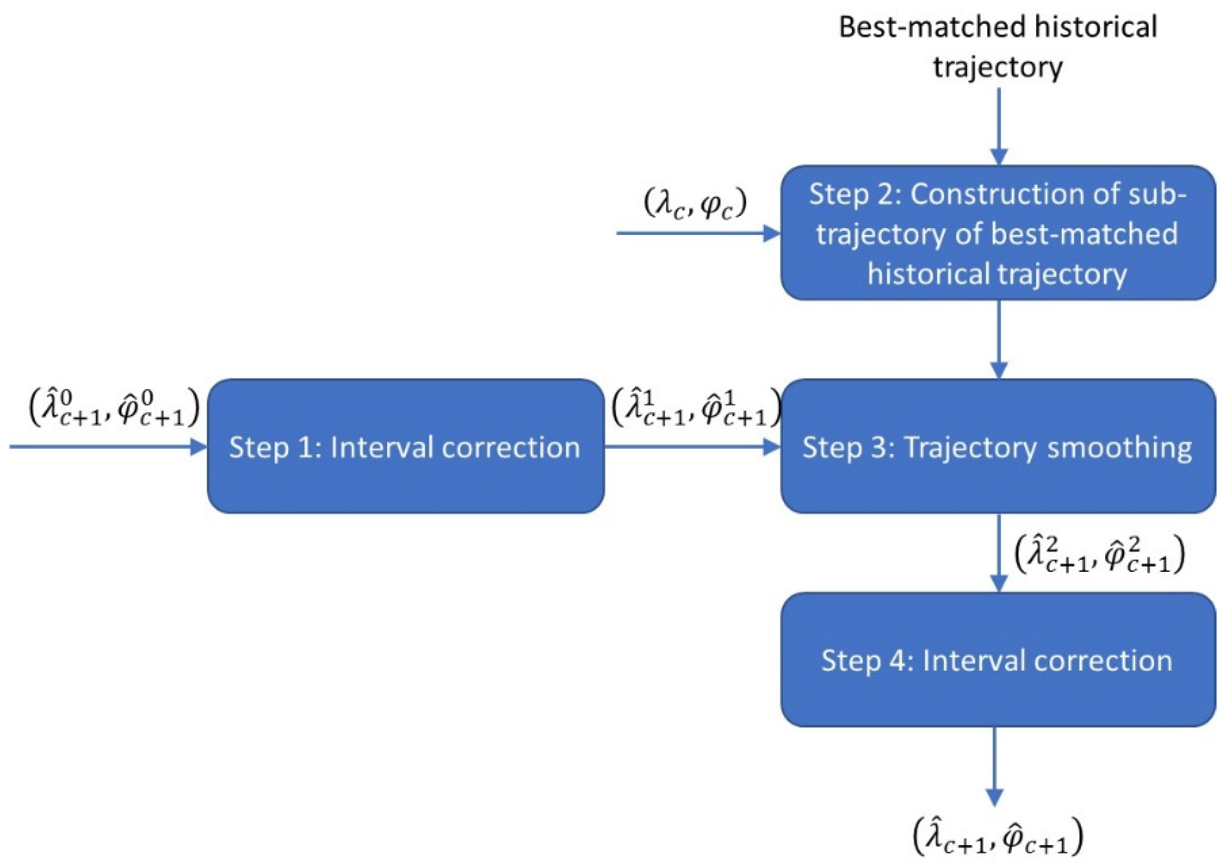
The construction layer consisted of four procedural steps, as shown in
Figure 6. Suppose the output of the dense layer is
. In the first step, an interval correction procedure was employed to adjust
and
so to have the GCD between the current position
and the adjusted prediction position, denoted by
, equal to
nm. In the second step, we constructed a sub-trajectory of the best-matched historical trajectory obtained in
Section 2.3 for the purpose of trajectory prediction smoothing. To illustrate how this is achieved, let us use
to denote the reconstructed trajectory point sequence of the best-matched historical trajectory (we use superscript
to represent the ”best-matched trajectory” in this paper). We “virtually” insert (
) into the point sequence of
, in the position right after the point closest to (
). The sub-trajectory is an artificial trajectory starting from (
) and connecting to the subsequent points in the sequence till the end of
. To ensure equal-distance separation, the points are further reconstructed following the same procedure in
Section 2.3.1, so that starting from (
), the subsequent reconstructed points are
nm apart. The resulting sub-trajectory is denoted by
where
and
for
(subscript
means the best-matched trajectory; subscript
means the remaining trajectory after the current position). In the third step, a smoothing procedure using
was applied to
, leading to updated longitude and latitude
. Finally, in the fourth step, the interval correction procedure was again employed, now to
, to ensure that the predicted point
is
nm apart from point
after smoothing. The output is
. Based on
,
is also calculated. Thus,
is generated. Below, we describe the interval correction and smoothing procedures in detail.
The interval correction procedure works as follows: Again, consider the output of the dense layer to be
. As the GCD between (
) and
may not be the prespecified separation distance of
nm, the interval correction procedure makes an adjustment by identifying the trajectory point that is
nm from
toward
. To this end, we first identify the tracking angle
clockwise from true north between
and
(
Figure 7).
Keeping the tracking angle
fixed, the longitude and latitude of the corrected point
are calculated using Equations (9)–(11) [
34], where
is the Earth’s radius.
For the smoothing procedure, as the LSTM model was trained based on a number of historical trajectories, our experiments show that some “zigzags” can occur to the predicted trajectories, which is not consistent with the real-world flying behavior. To mitigate this, we employed a procedure through which the LSTM-predicted trajectory is smoothed with the sub-trajectory of the best-matched historical trajectory. Specifically, for the th predicted trajectory point from the current flight position , the smoothed longitude and latitude () are calculated using Equations (12)–(14). In Equation (12), is the smoothing coefficient as the ratio of GCDs from the th predicted trajectory point and from the current flight position to the destination airport (). The farther the prediction is (i.e., larger ), the smaller the value of and consequently . With , the smoothed longitude of the th predicted trajectory point is . The rationale is that when the LSTM prediction gets farther into the future, more prediction errors can accumulate, making the prediction less reliable. As a result, less weight is given to the LSTM prediction and more reliance on the best-matched trajectory .
A potential issue with using
is that when the predicted trajectory point is near the destination airport, the role of LSTM will diminish to zero. To still have LSTM play a role in prediction, we took an additional weighted sum of
and the LSTM prediction
, weighted by
and
.
indicates the extent of using smoothing.
means no smoothing.
corresponds to full smoothing.
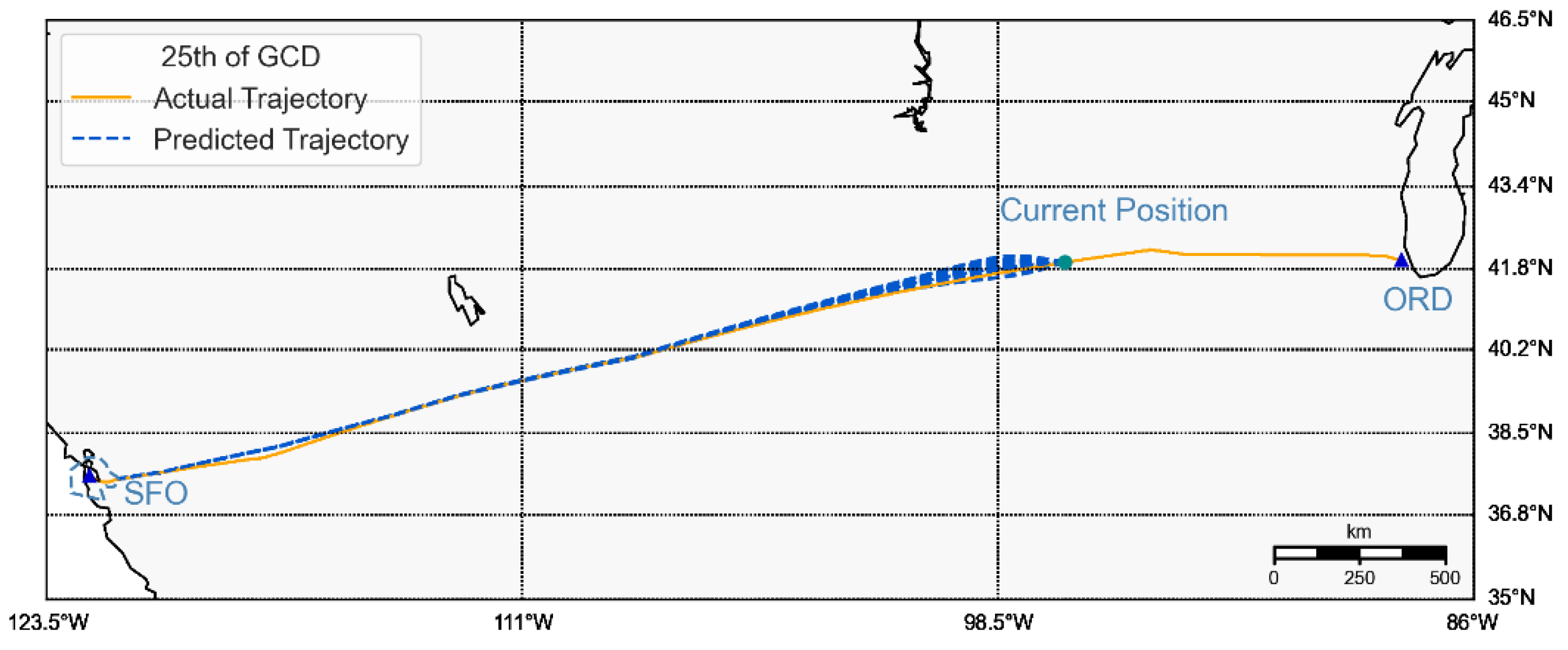
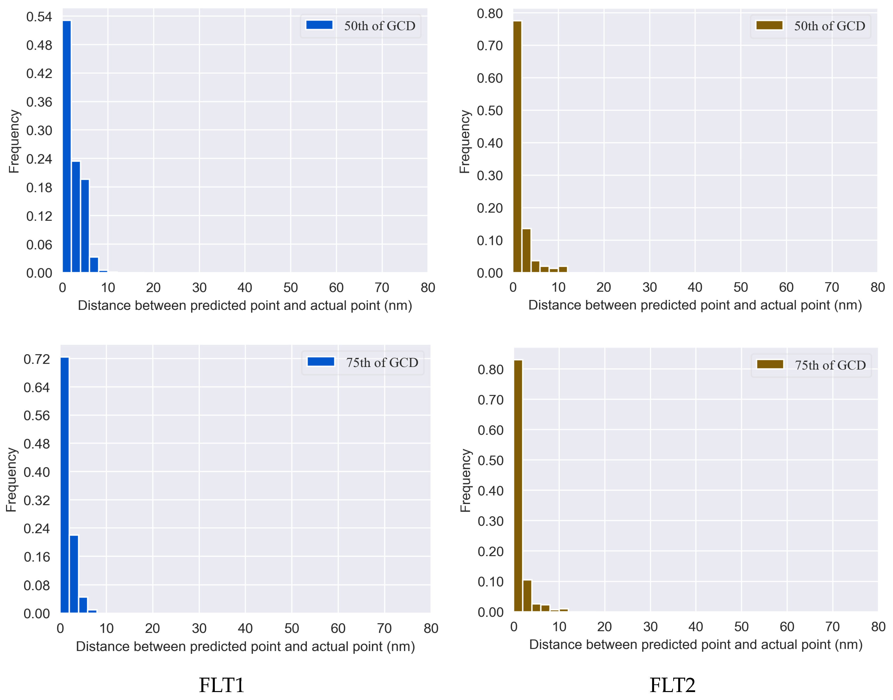
The above prediction procedure iteratively generated future trajectory points, until we identified the first trajectory point that reached the boundary of the destination terminal airspace or fell within the boundary (
Figure 8). Considering the random initialization of the weights of the LSTM neural network, a different model may be obtained each time we train the LSTM neural network using the same training data, which may result in a different trajectory. To account for the randomness, multiple LSTM models were trained for each historical trajectory. Thus, multiple predictions were performed, each corresponding to one trained LSTM model and generating one predicted trajectory.
As a final note, the way the LSTM-predicted trajectory points were adjusted is based on equal distance separation for trajectory points. As opposed to this, there would be a lack of basis for adjusting the LSTM-predicted trajectory points if they are required to be of equal time separation. This is because a predicted trajectory point is defined by longitude, latitude, and
, but not time or speed information. Even if speed were part of the LSTM prediction, the predicted trajectory point location and speed may result in a time separation different from the prespecified time interval between the predicted and its preceding trajectory points (to our knowledge, there is no way to force the time separation computed based on the LSTM-predicted trajectory point location and speed to be equal to the prespecified time separation). Therefore, time separation inconsistency can occur. This, along with the way raw trajectory points were reconstructed, as explained in
Section 2.3.1, justified the consideration of equal distance separation.


