
Research on Pilot Control Strategy and Workload for Tilt-Rotor Aircraft Conversion Procedure

Abstract
:1. Introduction
2. Flight Dynamics Model of XV-15 Tilt-Rotor Aircraft
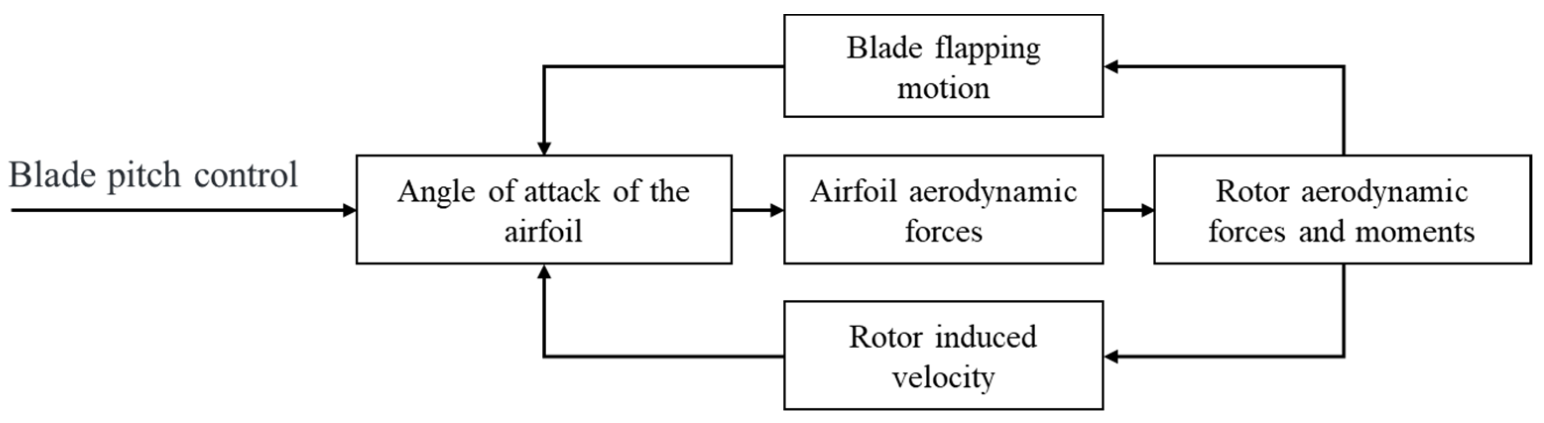
2.1. Modelling
2.2. Validation
3. Formulation of Nonlinear Optimal Control Problem
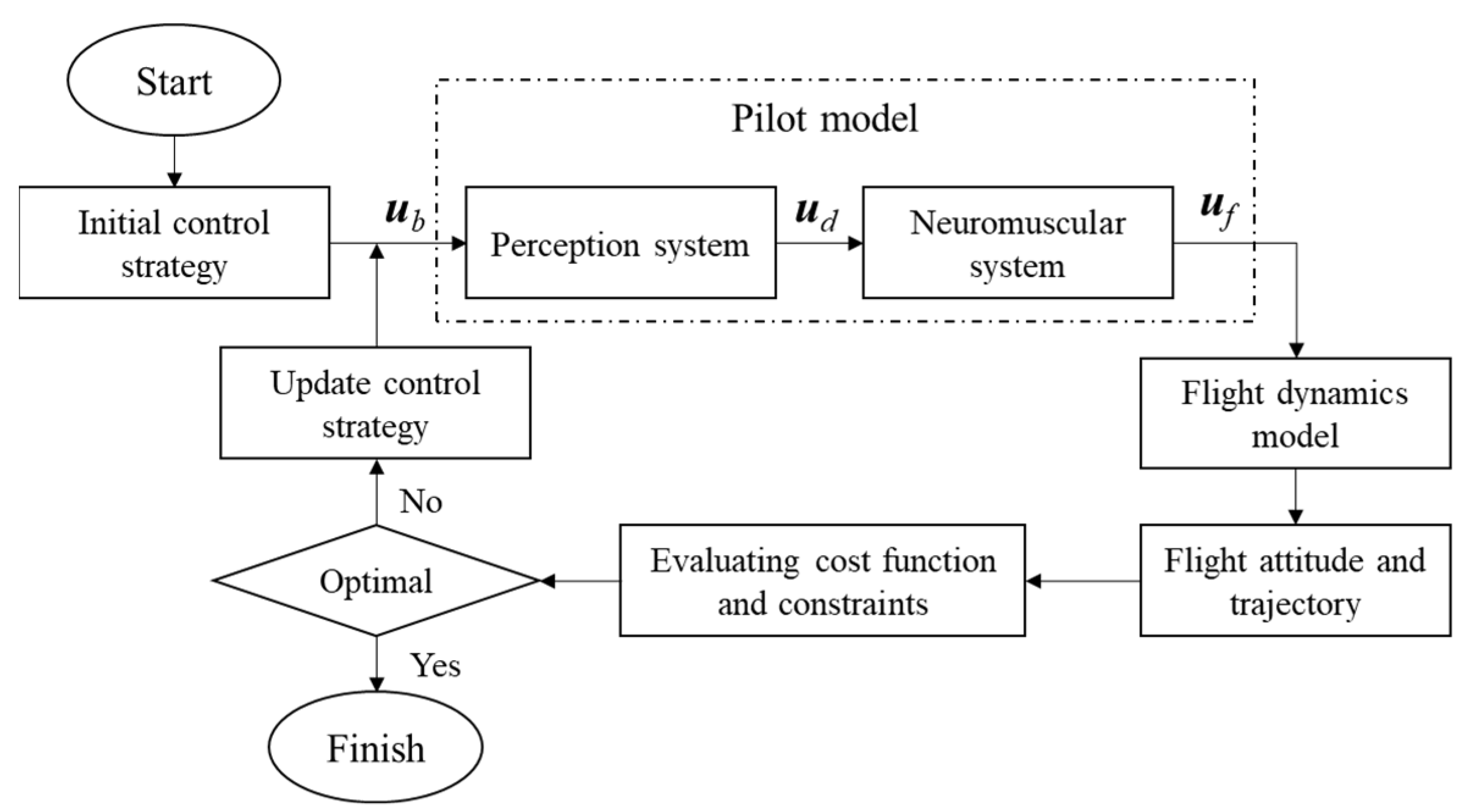
3.1. Pilot Model
3.2. Nonlinear Optimal Control Problem
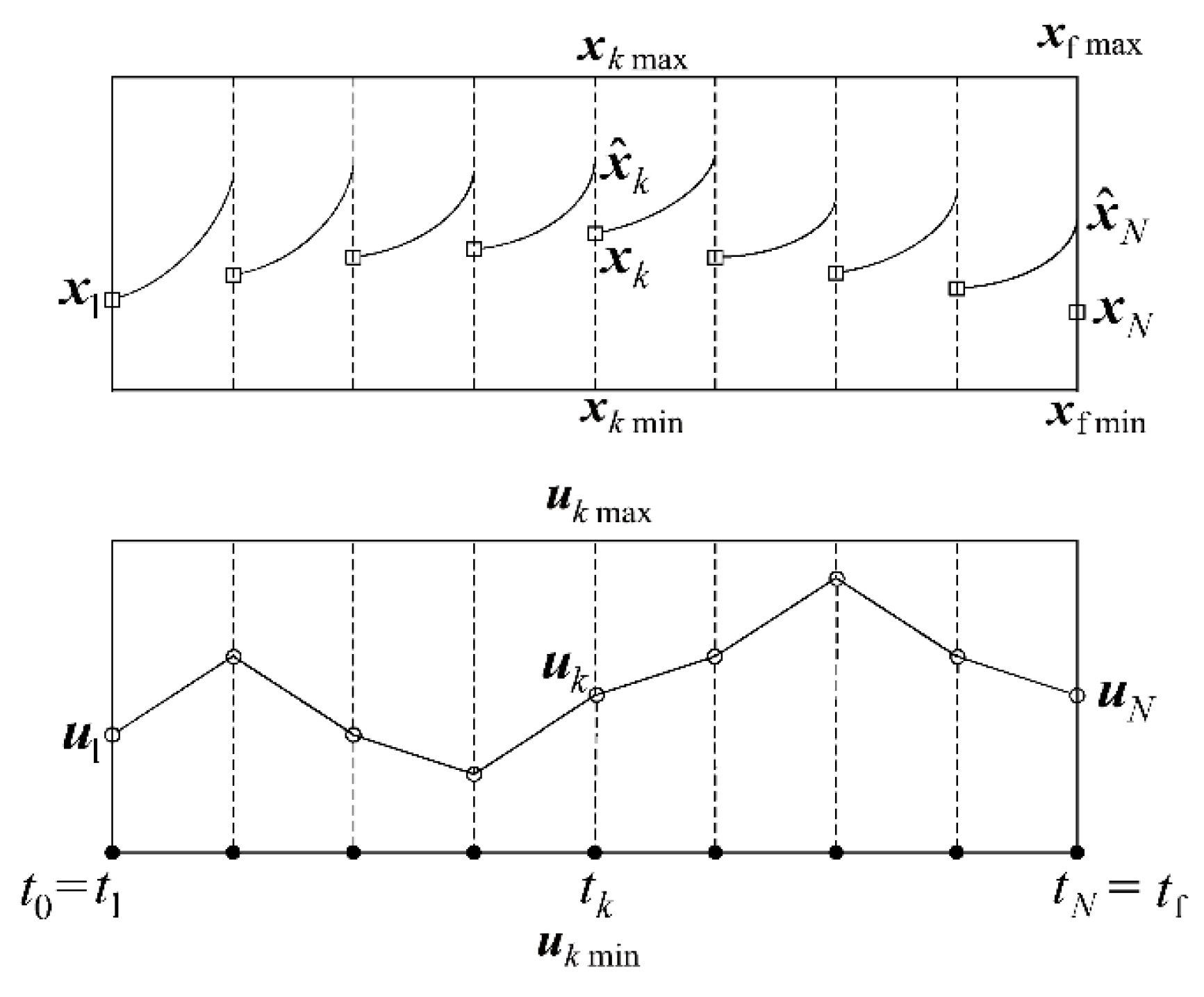
3.3. Numerical Solution Techniques
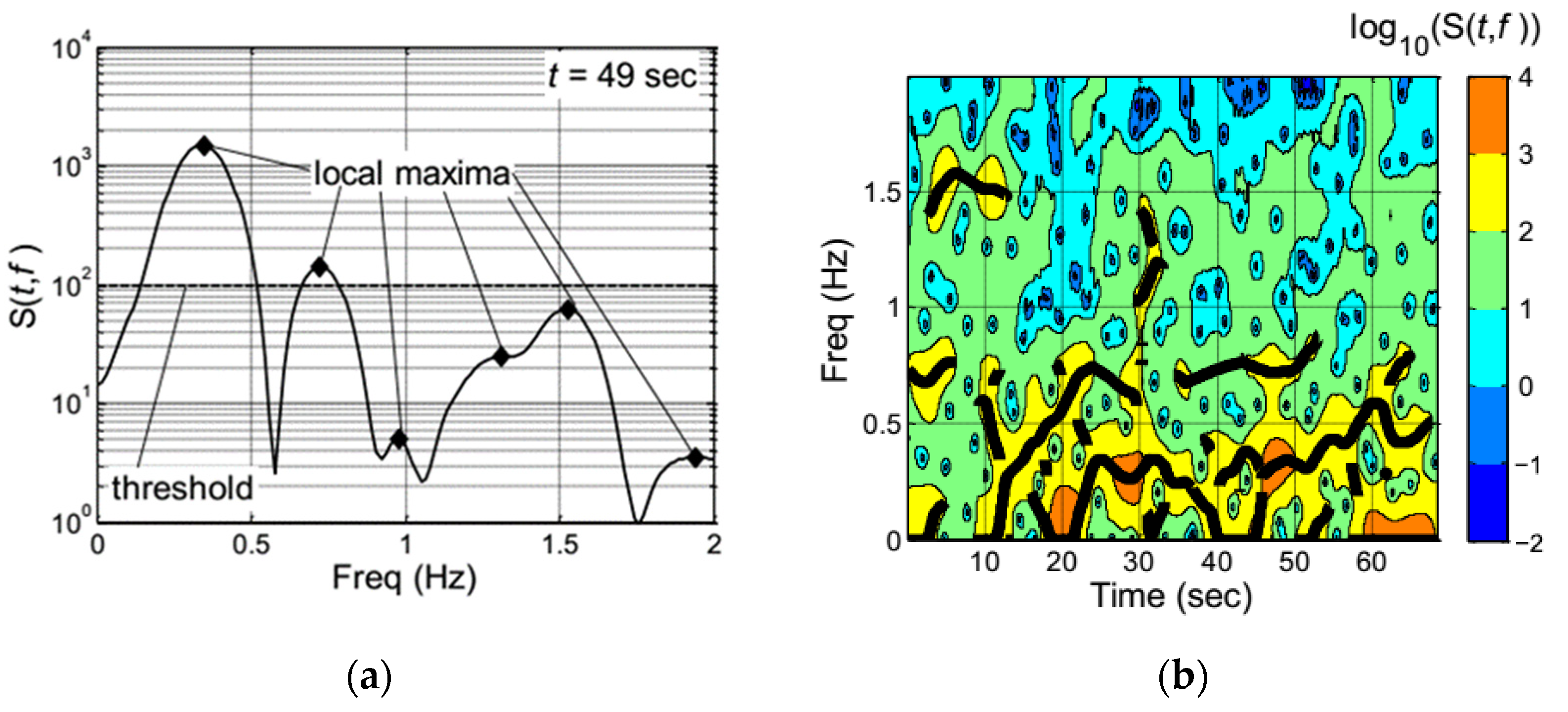
4. Workload Evaluation Method Based on Wavelet Analysis
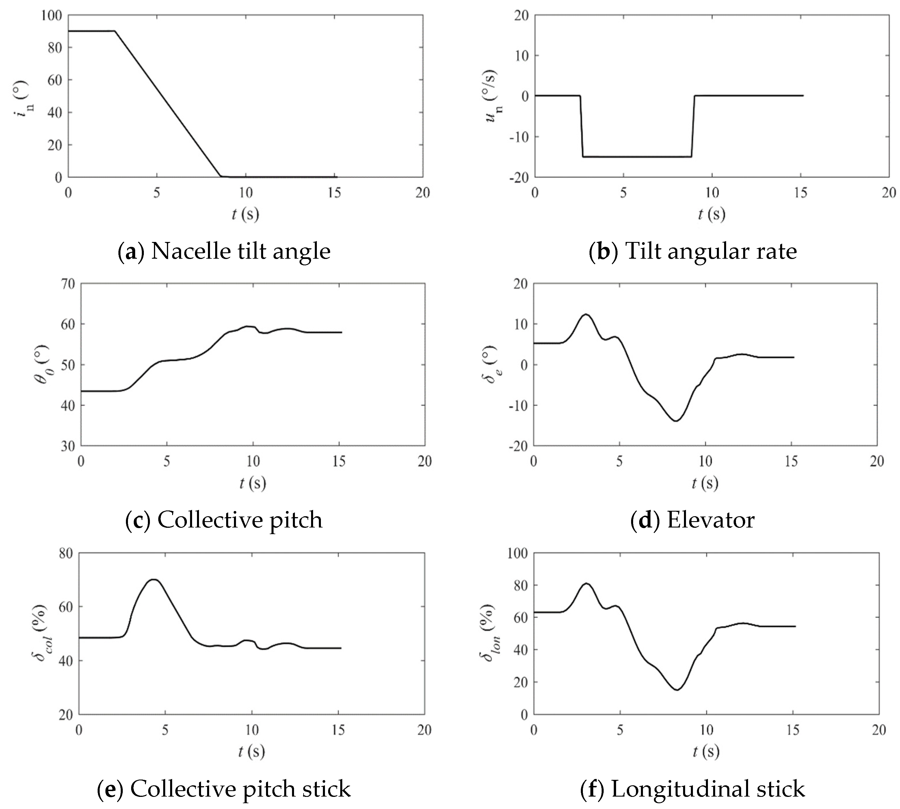
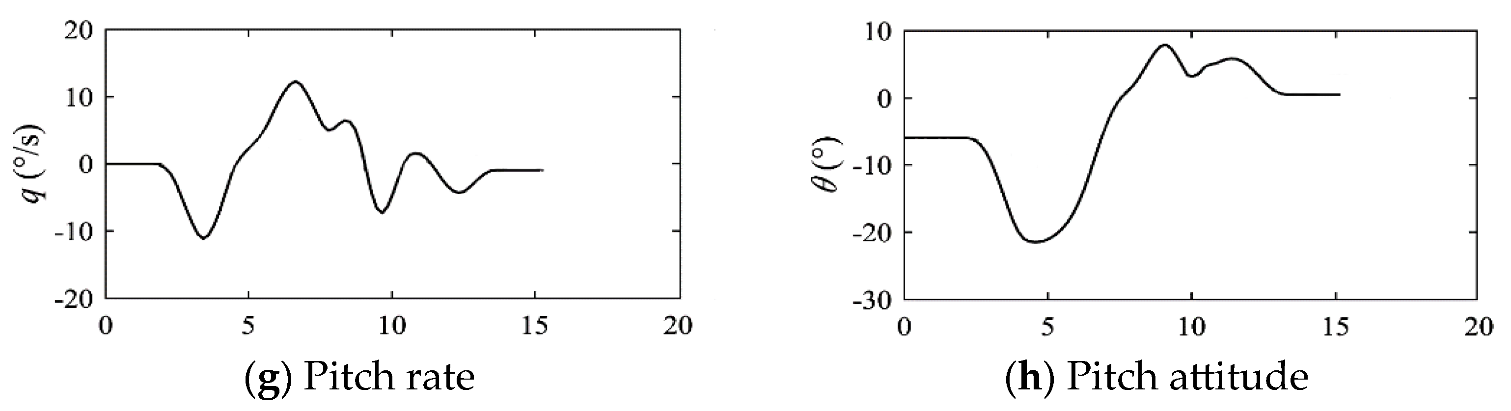
5. Tilt-Rotor Aircraft Forward Conversion Procedure
5.1. Task Description
5.2. Benchmark Performance Index
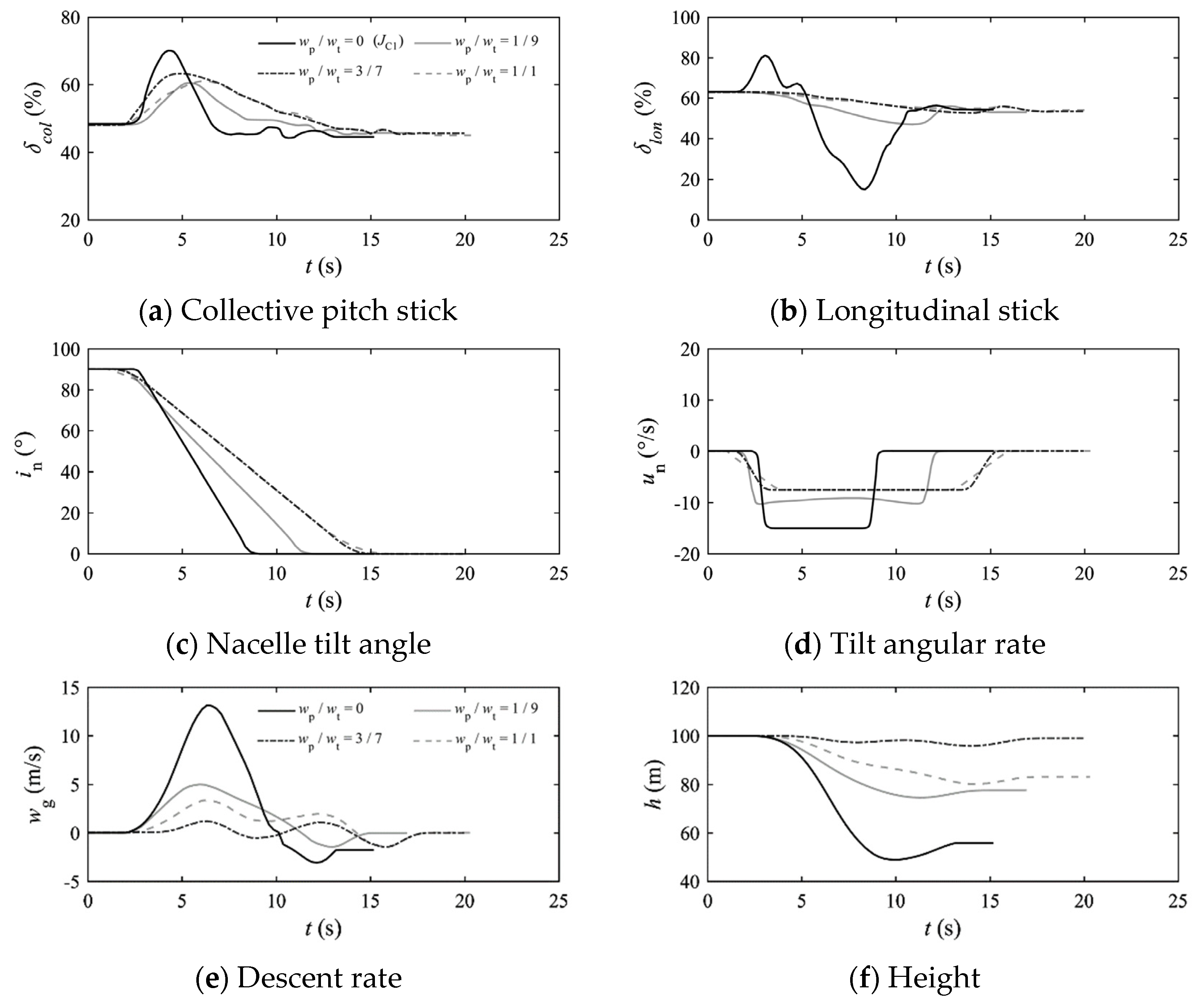
5.3. Weighting of Pilot Workload in Performance Index
6. Tilt-Rotor Aircraft Backward Reconversion Procedure
6.1. Task Description
6.2. Benchmark Performance Index
6.3. Weighting of Pilot Workload in Performance Index
7. Conclusions
8. Future Works
Author Contributions
Funding
Data Availability Statement
Conflicts of Interest
Abbreviations
| List of abbreviations | |
| NOCP | Nonlinear optimal control problem |
| HQR | Handling quality rating |
| PIO | Pilot-induced oscillation |
| TFRs | Time-frequency representations |
| GTRS | Generic tilt-rotor aircraft simulation |
| NLP | Nonlinear programming |
| SQP | Series quadratic programming |
| STFT | Short-time Fourier transform |
| PSD | Power spectral density |
| db | Daubechies |
| MTE | Mission task element |
| List of symbols | |
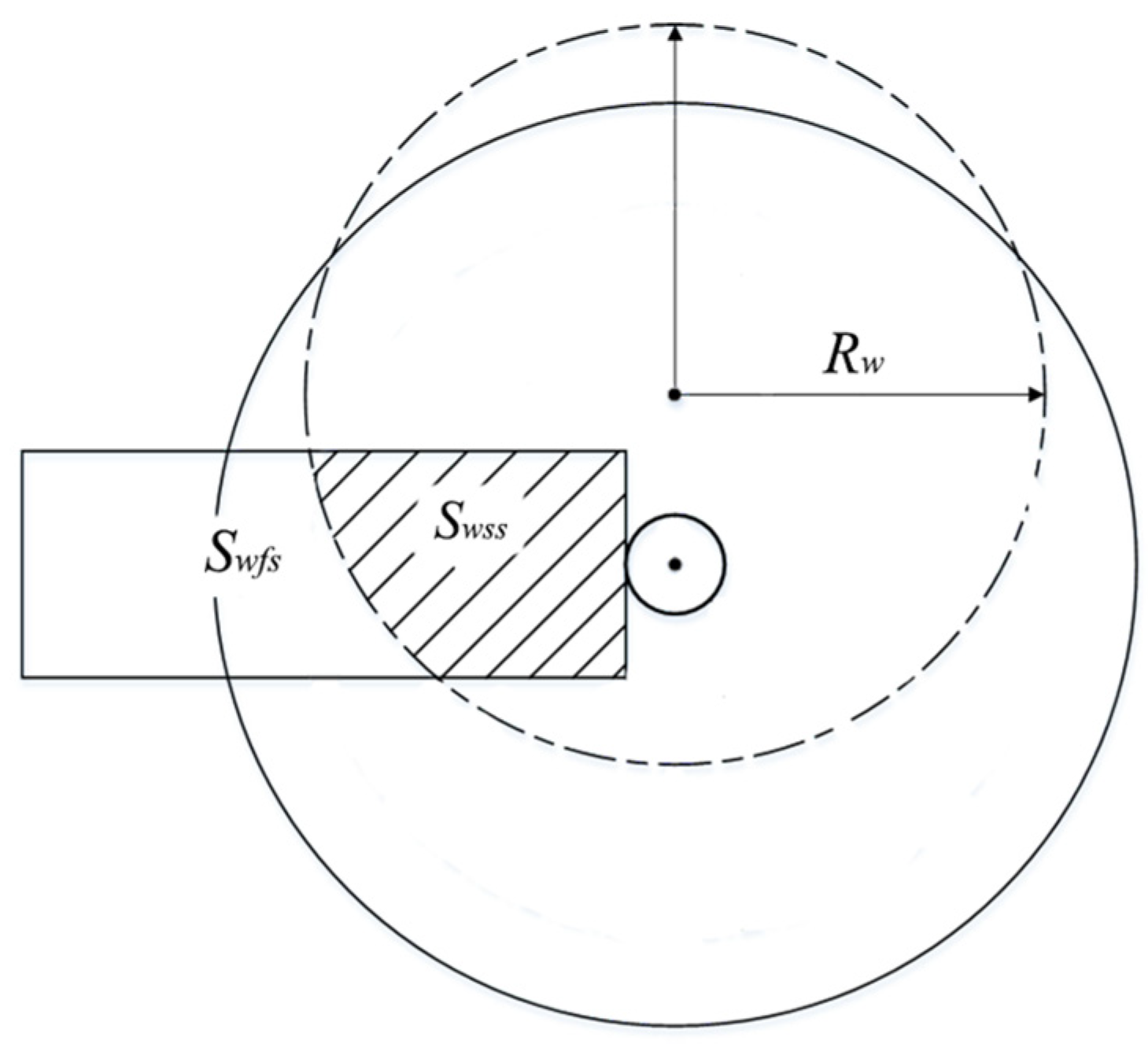
| Swfs | Wing area in the free stream |
| Swss | Wing area in the rotor slipstream |
| Rw | Contracted wake radius |
| Fuselage state, rotor state, inflow state | |
| Collective stick input, lateral stick input, longitudinal stick input, pedal input, nacelle tilting angle | |
| Linear velocities of the aircraft body axis system | |
| Angular velocities of the body axis system | |
| Roll, pitch, and yaw angles, respectively | |
| Position of the aircraft in the Earth axis system | |
| Taper, rear, and side angles of the rotor disk, respectively | |
| Non-dimensional terms for rotor uniform inflow, first-order cosine inflow, and first-order sine inflow, respectively | |
| Perception system and neuromuscular system | |
| TL, TI, TN, τp | Feedforward time constant, lag time constant, neuromuscular response time, and delay time, respectively |
| ud, uf | Delayed command inputs and final control input, respectively |
| xp | Relevant state variables of the neuromuscular system |
| A, B, C, D | Matrices of the pilot model in the state-space form |
| Control rates | |
| Wing angle of attack | |
| Required and rated power output of the engine (two), respectively | |
| Ω0 | Standard main rotor rotational speed |
| k1~k4 | Constant scaling factors |
| , | Number of cycles and frequency, respectively |
| Wavelet function | |
| Weighted power | |
| Wavelet coefficient | |
| , | Performance indices for forward conversion |
| , | Performance indices for backward reconversion |
| wt, wp | Time weighting coefficient and pilot control workload weighting coefficient, respectively |
| wcol, wlon, wn | Weighting coefficients for the corresponding control rates |
References
- Yuan, Y.; Thomson, D.; Anderson, D. Application of Automatic Differentiation for Tilt-Rotor Aircraft Flight Dynamics Analysis. J. Aircr. 2020, 57, 985–990. [Google Scholar] [CrossRef]
- Xufei, Y.; Renliang, C. Augmented flight dynamics model for pilot workload evaluation in tilt-rotor aircraft optimal landing procedure after one engine failure. Chin. J. Aeronaut. 2019, 32, 92–103. [Google Scholar] [CrossRef]
- Padfield, G.D. Helicopter Flight Dynamics: Including a Treatment of Tiltrotor Aircraft, 3rd ed.; John Wiley & Sons: New York, NY, USA, 2018; pp. 154–196. [Google Scholar]
- Nabi, H.; De, V.C.; Pavel, M.D.; Delft University of Technology and Politecnico di Milano. A quasi-linear parameter varying (qlpv) approach for tiltrotor conversion modeling and control synthesis. In Proceedings of the American Helicopter Society 75th Annual Forum, AHS, Philadelphia, PA, USA, 13–16 May 2019; pp. 1–12. [Google Scholar]
- Yan, X.; Chen, R.; Lou, B.; Xie, Y.; Xie, A.; Zhang, D. Study on control strategy for tilt-rotor aircraft conversion procedure. J. Phys. Conf. Ser. 2021, 1924, 012010. [Google Scholar] [CrossRef]
- Yeo, H.; Saberi, H. Tiltrotor conversion maneuver analysis with RCAS. J. Am. Helicopter Soc. 2021, 66, 1–14. [Google Scholar] [CrossRef]
- Righetti, A.; Muscarello, V.; Quaranta, G. Linear parameter varying models for the optimization of tiltrotor conversion maneuver. In Proceedings of the American Helicopter Society 73th Annual Forum, AHS, Fort Worth, TX, USA, 9–11 May 2017; pp. 280–287. [Google Scholar]
- Memon, W.A.; White, M.D.; Padfield, G.D.; Cameron, N.; Lu, L. Helicopter Handling Qualities: A study in pilot control compensation. Aeronaut J. 2022, 126, 152–186. [Google Scholar] [CrossRef]
- Lampton, A.; Klyde, D.H. Power frequency: A metric for analyzing pilot-in-the-loop flying tasks. J. Guid. Control Dynam. 2012, 35, 1526–1537. [Google Scholar] [CrossRef]
- Klyde, D.H.; Pitoniak, S.P.; Schulze, P.C.; Ruckel, P.; Rigsby, J.; Fegely, C.E.; Xin, H.; Fell, W.C.; Brewer, R.; Conway, F.; et al. Piloted simulation evaluation of tracking mission task elements for the assessment of high-speed handling qualities. J. Am. Helicopter Soc. 2020, 65, 1–23. [Google Scholar] [CrossRef]
- Tritschler, J.K.; O’Connor, J.C.; Holder, J.M.; Klyde, D.H.; Lampton, A.K. Interpreting time-frequency analyses of pilot control activity in ADS-33E mission task elements. In Proceedings of the American Helicopter Society 73rd Annual Forum, AHS, Fort Worth, TX, USA, 9–11 May 2017. [Google Scholar]
- Tritschler, J.K.; O’Connor, J.C.; Klyde, D.H.; Lampton, A.K. Analysis of pilot control activity in ADS-33e mission task elements. In Proceedings of the American Helicopter Society 72th Annual Forum, AHS, West Palm Beach, FL, USA, 17–19 May 2016; pp. 150–174. [Google Scholar]
- Mello, R.S.; Klyde, D.H.; Mitchell, D.G. Aircraft Accident Investigation Using Wavelet Scalogram-Based Metric to Identify Possible PIO Signature. In Proceedings of the AIAA SCITECH 2023 Forum, AIAA, National Harbor, MD & Online, 23–27 January 2023; p. 1367. [Google Scholar] [CrossRef]
- Ji, H.; Chen, R.; Li, P. Real-time simulation model for helicopter flight task analysis in turbulent atmospheric environment. Aerosp. Sci. Technol. 2019, 92, 289–299. [Google Scholar] [CrossRef]
- Ferguson, S.W. A Mathematical Model for Real Time Flight Simulation of a Generic Tilt-Rotor Aircraft; Technical Report: CR-166536; NASA Ames Research Center: Mountain View, CA, USA, 1988.
- Ferguson, S.W. Development and Validation of a Simulation for a Generic Tilt-Proprotor Aircraft; Technical Report: CR-166537; NASA Ames Research Center: Mountain View, CA, USA, 1989; pp. A1–A185.
- Carlo, L.; Bottasso, G.; Francesco, S. Trajectory Optimization Procedures for Rotorcraft Vehicles Including Pilot Models, with Applications to ADS-33 MTEs, Cat-A and Engine off Landings. In Proceedings of the American Helicopter Society 65th Annual Forum and Technology Display, AHS, Grapevine, TX, USA, 27–29 May 2009; pp. 1–14. [Google Scholar]
- Calise, A.J.; Rysdyk, R. Research in Nonlinear Flight Control for Tiltrotor Aircraft Operating in the Terminal Area; Technical Report: CR-203112; NASA: Washington, DC, USA, 1996.
- An, K.; Guo, Z.-Y.; Xu, X.-P.; Huang, W. A framework of trajectory design and optimization for the hypersonic gliding vehicle. Aerosp. Sci. Technol. 2020, 106, 106110. [Google Scholar] [CrossRef]
- Jin, R.; Huo, M.; Xu, Y.; Zhao, C.; Yang, L.; Qi, N. Rapid cooperative optimization of continuous trajectory for electric sails in multiple formation reconstruction scenarios. Aerosp. Sci. Technol. 2023, 140, 108385. [Google Scholar] [CrossRef]
- Yan, X.; Chen, R.; Zhu, S.; Xie, A.; Gu, J. Optimal Landing of Tilt-rotor Aircraft after Engine Failure Considering Pilot Inherent Limitations. In Proceedings of the 2022 IEEE International Conference on Robotics and Biomimetics (ROBIO), IEEE, Jinghong, China, 5–9 December 2022; pp. 1036–1040. [Google Scholar] [CrossRef]
- Yu, X.; Chen, R.; Wang, L.; Yan, X.; Yuan, Y. An optimization for alleviating pilot workload during tilt rotor aircraft conversion and reconversion maneuvers. Aerosp. Sci. Technol. 2022, 129, 107854. [Google Scholar] [CrossRef]
- Zhiming, Y.; Xufei, Y.; Renliang, C. Prediction of pilot workload in helicopter landing after one engine failure. Chin. J. Aeronaut. 2020, 33, 3112–3124. [Google Scholar] [CrossRef]
- Gossler, F.E.; Oliveira, B.R.; Duarte, M.A.Q.; Filho, J.V.; Villarreal, F.; Lamblém, R.L. Gaussian and Golden Wavelets: A Comparative Study and their Applications in Structural Health Monitoring. Trends Comput. Appl. Math. 2021, 22, 139–155. [Google Scholar] [CrossRef]
- Da Silva, P.C.L.; Da Silva, J.P.; Garcia, A.R.G. Daubechies wavelets as basis functions for the vectorial beam propagation method. J. Electromagnet Wave. 2019, 33, 1027–1041. [Google Scholar] [CrossRef]


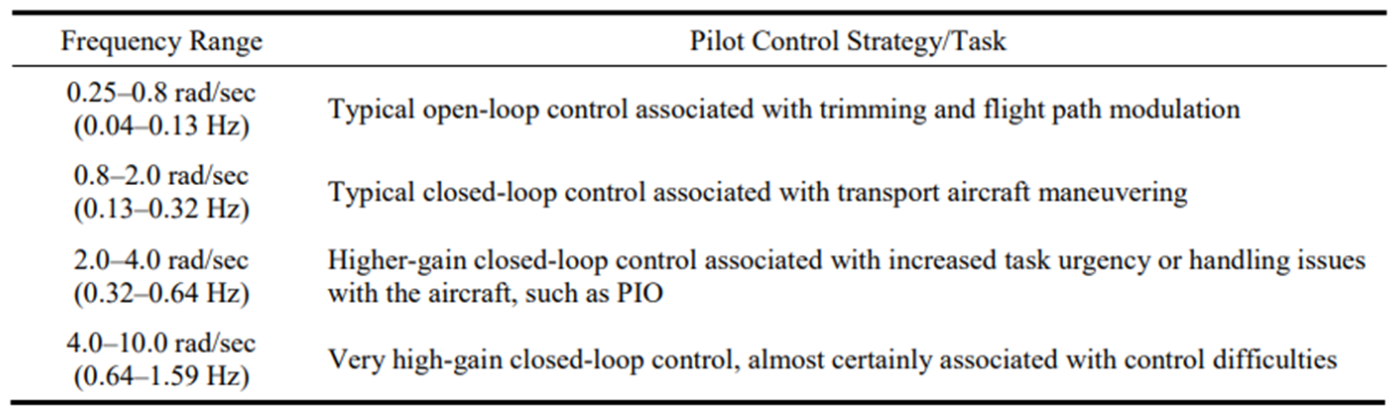
| Dominant Frequency Range | Pilot Control Strategy/Task | HQR Scale |
|---|---|---|
| 0.25–0.8 rad/s (0.04–0.13 Hz) | Typical open-loop control associated with trimming and flight path modulation | Level 1 (1~3) |
| 0.8–2.0 rad/s (0.13–0.32 Hz) | Typical closed-loop control associated with transport aircraft maneuvering | Level 2 (4~6) |
| 2.0–4.0 rad/s (0.32–0.64 Hz) | Higher-gain, closed-loop control associated with increased task urgency or handling issues with the aircraft, such as PIO | Level 3 (7~9) |
| 4.0–10.0 rad/s (0.64–1.59 Hz) | Very high-gain, closed-loop control almost certainly associated with control difficulties | 10 |
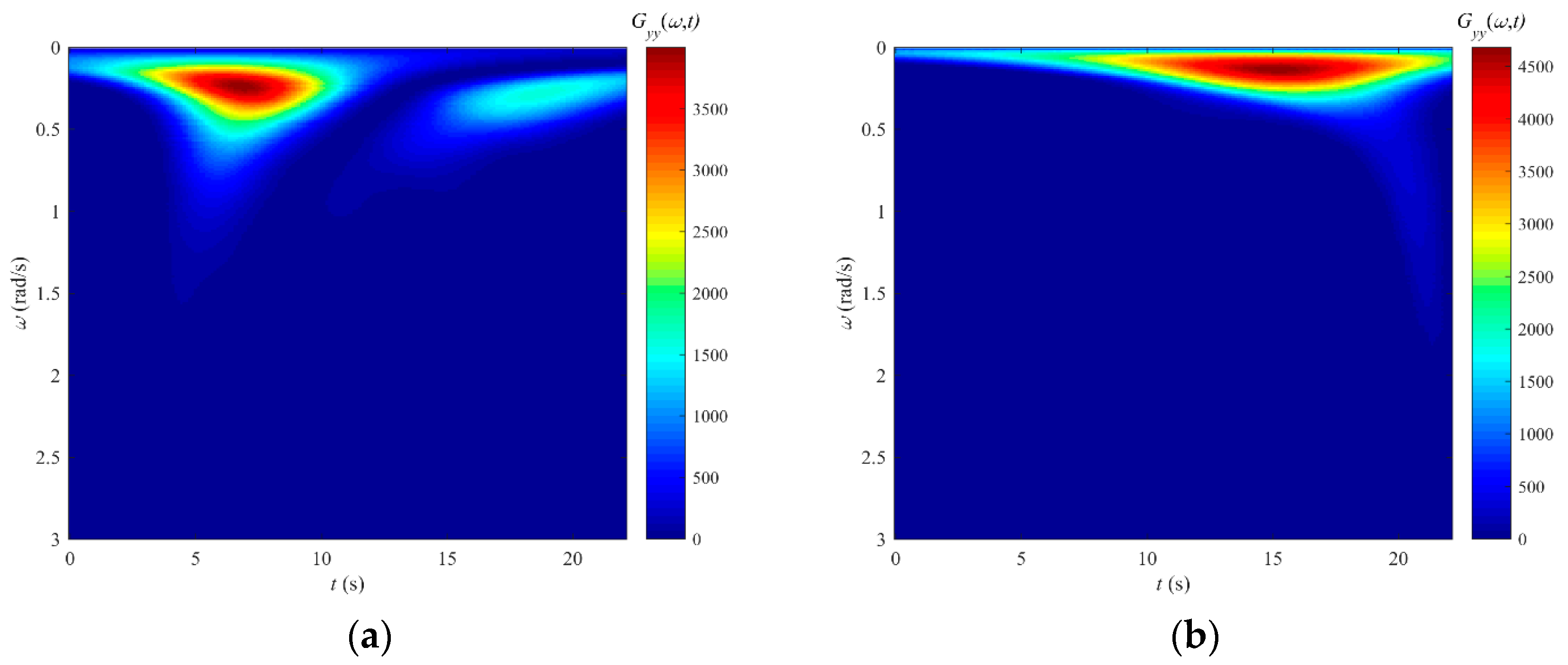
| Control | Item | Figure 14 | Figure 16 |
|---|---|---|---|
| Collective pitch stick | Dominant frequency components | 0.2~2.0 rad/s, ~2.0 rad/s | 0.1~0.8 rad/s, <1.6 rad/s |
| Maximum energy | 4500%2/(rad/s) | 3900%2/(rad/s) | |
| Longitudinal stick | Dominant frequency components | 0.1~1.5 rad/s, ~2.0 rad/s | 0.1~0.8 rad/s, <1.8 rad/s |
| Maximum energy | 23,000%2/(rad/s) | 4600%2/(rad/s) |
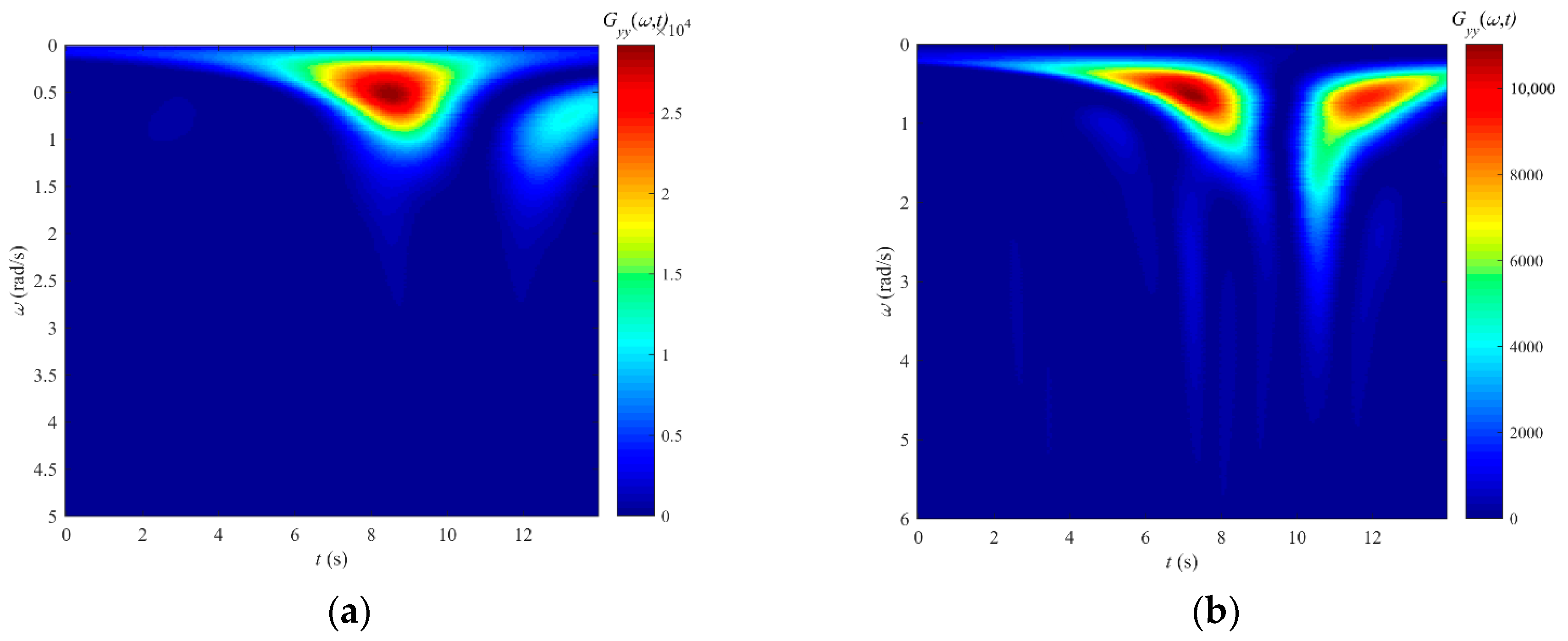
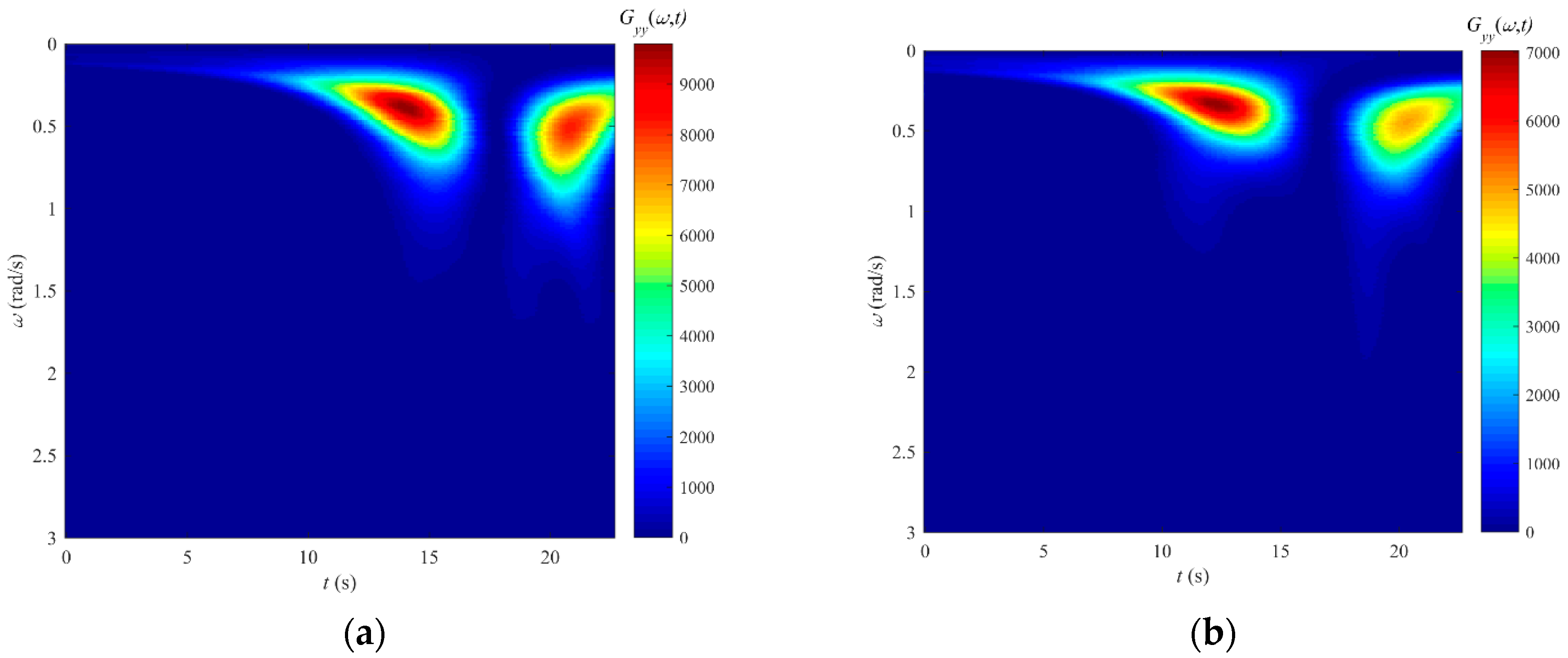
| Control | Item | Figure 18 | Figure 20 |
|---|---|---|---|
| Collective pitch stick | Dominant frequency components | 0.1~2.0 rad/s | 0.2~0.8 rad/s, <1.7 rad/s |
| Maximum energy | 29,000%2/(rad/s) | 9800%2/(rad/s) | |
| Longitudinal stick | Dominant frequency components | 0.2~4 rad/s | 0.2~0.8 rad/s, <2.0 rad/s |
| Maximum energy | 11,000%2/(rad/s) | 7000%2/(rad/s) |
Disclaimer/Publisher’s Note: The statements, opinions and data contained in all publications are solely those of the individual author(s) and contributor(s) and not of MDPI and/or the editor(s). MDPI and/or the editor(s) disclaim responsibility for any injury to people or property resulting from any ideas, methods, instructions or products referred to in the content. |
© 2023 by the authors. Licensee MDPI, Basel, Switzerland. This article is an open access article distributed under the terms and conditions of the Creative Commons Attribution (CC BY) license (https://creativecommons.org/licenses/by/4.0/).
Share and Cite
Yan, X.; Yuan, Y.; Chen, R. Research on Pilot Control Strategy and Workload for Tilt-Rotor Aircraft Conversion Procedure. Aerospace 2023, 10, 742. https://doi.org/10.3390/aerospace10090742
Yan X, Yuan Y, Chen R. Research on Pilot Control Strategy and Workload for Tilt-Rotor Aircraft Conversion Procedure. Aerospace. 2023; 10(9):742. https://doi.org/10.3390/aerospace10090742
Chicago/Turabian StyleYan, Xufei, Ye Yuan, and Renliang Chen. 2023. "Research on Pilot Control Strategy and Workload for Tilt-Rotor Aircraft Conversion Procedure" Aerospace 10, no. 9: 742. https://doi.org/10.3390/aerospace10090742