Article

Discretization Method to Improve the Efficiency of Complex Airspace Operation

1
College of Air Traffic Management, Civil Aviation Flight University of China, Guanghan 618307, China
2
Northeast Regional Air Traffic Management Bureau of CAAC, Shenyang 110046, China
*
Authors to whom correspondence should be addressed.
Aerospace 2023, 10(9), 780; https://doi.org/10.3390/aerospace10090780
Submission received: 25 May 2023 / Revised: 20 August 2023 / Accepted: 21 August 2023 / Published: 1 September 2023
(This article belongs to the Section Air Traffic and Transportation)

Abstract

:
With the increase in airspace flow, the complexity of the airspace operation environment has also increased. Against this backdrop, improving the operational efficiency of airspace is crucial to ensure its efficient operation. The discrete division of controlled airspace represents a novel methodology for achieving this end. This approach involves visualizing the use of the airspace, quantifying and evaluating the operational efficiencies of airspace environments, and assessing specific metrics during an allocated time period. In this study, a discrete unit model was constructed to hierarchically subdivide complex airspace into static obstacles and aircraft-occupied space units, which facilitated the optimization of decision-making operations for multiple aircraft in airspace using the discrete method. Furthermore, busy airspace units could be effectively avoided. Finally, by using the extended analytic hierarchy process, we evaluated the threshold value of airspace operational efficiency improvement when operation efficiency metrics were enhanced via discrete approaches. The results indicated that the threshold value was 0.02168, classified as “good”, which represented an improvement in comparison with the original value of airspace operational efficiency (0.03173). These findings demonstrated that the application of the discrete division methodology significantly improved the overall operational efficiency of the airspace.

1. Introduction

With the increase in airspace flow, airspace operation becomes more complex. It is of great significance to improve the efficiency of airspace operation. In this paper, a discretization method is used to divide the airspace with obstacles and complex situations into different levels and to quantify and evaluate the performance of the Operational Efficiency Index of the complex airspace. It provides a new method to solve the problem of low efficiency of airspace operation. These optimization methods will drive the expansion of a dynamic airspace management framework that integrates air and space, thereby improving airspace operational efficiency. To address issues such as irrational airspace structures and poor coordination among airspace operations, inter-unit coordination and communication within control units should be strengthened in the short term, and a complete coordination mechanism should be established in the long term. A digitized model based on discrete airspace units at the spatial level can be established to achieve this. The concept of the discrete grid originated from the two-dimensional flat grid system applied to the Earth [1]. As the development of geographic information technology required a method for the systematic management of geographic spatial data, a multilevel grid theory method was proposed [2]. The concept of spatial discretization is currently mainly used in aircraft trajectory planning, conflict resolution between aircraft, and dynamic airspaces. The application of discretization to traffic flow management is primarily reflected in air traffic flow prediction and the recording of all aircraft operational data. Additionally, it includes the use of regular hexahedron-based airspace performance analysis tools, dynamic airspace configuration methods, and techniques for dynamically configuring control sectors based on the evolution of air traffic flow [3,4]. Stankūnas proposed a new approach to solving the problem of European airspace’s low operating efficiency and studied the characteristics of air traffic flow in the airspace by subdividing the European airspace into six blocks based on air traffic flow and then determining the number of airspace grids in each block using hierarchical clustering methods [5]. Similarly, Kondroška addressed the issue of unit grid subdivision in European airspace. They assigned weight coefficients to the grids based on the number of times they were crossed by aircraft trajectories and used hierarchical clustering methods to divide the airspace into multiple airspace unit blocks, resulting in continuous horizontal flight paths for aircraft flying through the discrete airspace [6]. The FAA applied the discretization method to enhance traffic flow management by simulating different levels of aircraft trajectories using monotone Lagrange meshes, which enabled the prediction of air traffic distribution [7]. An et al. used a grid-based method to partition airspace and detected and transformed irregular shapes, such as restricted zones and obstacles, into regular ones. They then planned optimal flight routes using coordinate-based methods [8]. Wang transformed obstacles into grid areas of a certain size and used ant colony algorithms to calculate optimal aircraft routes [9]. Matthews mined and organized airport data, demonstrating inconsistencies between actual aircraft routes and planned trajectories, with different impacts on subsequent aircraft operations. They analyzed flights with similar abnormal positions during different time periods and compared their route planning paths [10]. Marina divided the spatial domain into different 3D spatial blocks, used a genetic algorithm to optimize the spatial configuration, and calculated the workload of different sector workers [11]. Gerdes et al. introduced a concept to map free routes to a routing system. They used clustering algorithms to identify major traffic flows for the assignment [12]. In 2020, he also introduced the concept of a free route, which directly connects the departure and destination airports to reduce the flight path length, and used clustering algorithms to identify major traffic flows for monitoring purposes [13]. Yang divided large amounts of spatiotemporal data into multiple grid cells according to the spatial domain they occupied and ranked and calculated spatial data storage occupation rates, aiming to minimize the use of data space [14]. The Single European Sky Implementation Plan applied discretization algorithms to a functional airspace block configuration using an inner ring algorithm to detect conflicts for each unit cell over discrete time steps [15]. Zhang analyzed the operational efficiency, safety, and economic indicators of complex airspaces, quantified an indicator system to evaluate the airspace use rate, and listed factors affecting airspace operations [16]. Wang proposed a method for evaluating the coefficients and relations of various indicators in airspace considering the complex characteristics of general aviation flight and low-altitude airspace environments by analyzing the number of aircraft and their speeds [17]. Miao proposed a low-altitude flight conflict detection algorithm based on spatiotemporal indexing. They discretized and recognized airspace, used GeoSOT to establish a multilevel grid index priority strategy, and detected path conflicts caused by complex low-altitude spatiotemporal changes. They improved the efficiency of conflict identification for one aircraft and the computational time for route planning [18]. With regard to research on the spatial discretization of airspace, constructing a grid identification system for airspace is crucial for the application of information technology in airspace management, promoting airspace digitization. Zhu et al. proposed the construction of discrete units for airspace, the establishment of a partition model for airspace altitude levels, and the accurate coding of discretized airspace, providing technological support for developing the next generation of airspace management. On this basis, the track planning of the digital airspace concept and the calculation of its space-time resources are verified [19,20]. Tluchor divided extremely low airspace and performed evaluations based on the operational risks of unmanned aerial vehicles [21]. The algorithms were based on an advanced bidirectional RRT∗algorithm that generated risk-minimizing flight paths with predefined flight times [22].
Discretizing airspace involves transforming traditional continuous airspace objects into gridded airspace objects to make better use of limited airspace, further optimize flight routes, and resolve dynamic airspace use problems. Applying the discretization method to optimize an airspace system lays the foundation for building a comprehensive aviation transportation network system with an optimal system layout and efficient operation.

2. Problem Analysis and Methods

Digital airspace refers to the use of mathematical models to characterize the structure of airspace, aircraft trajectories, and the airspace occupied by aircraft. This approach aims to solve the problem of low operational efficiency in complex airspace operations. The main research focus of this paper includes the following:
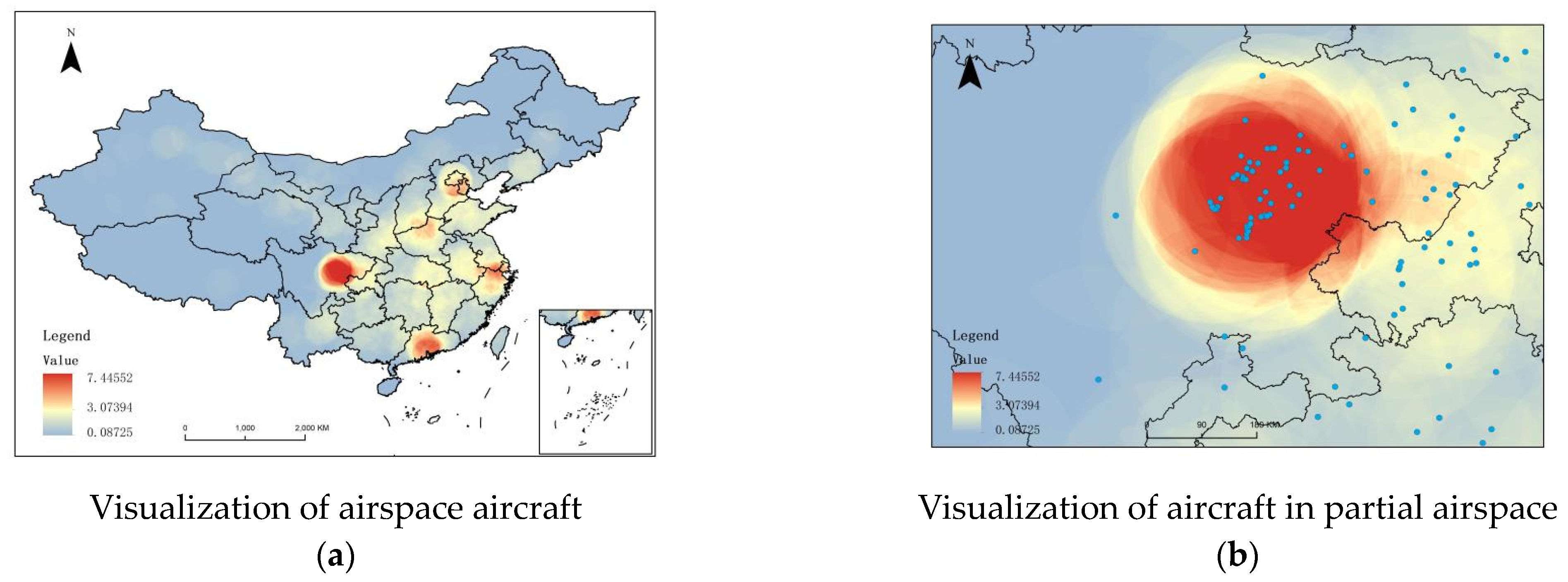
  • The visualization analysis of airspace is represented by a digital model that provides a numerical representation of the entire operation of the airspace, enabling researchers and controllers to clearly observe airspace use.
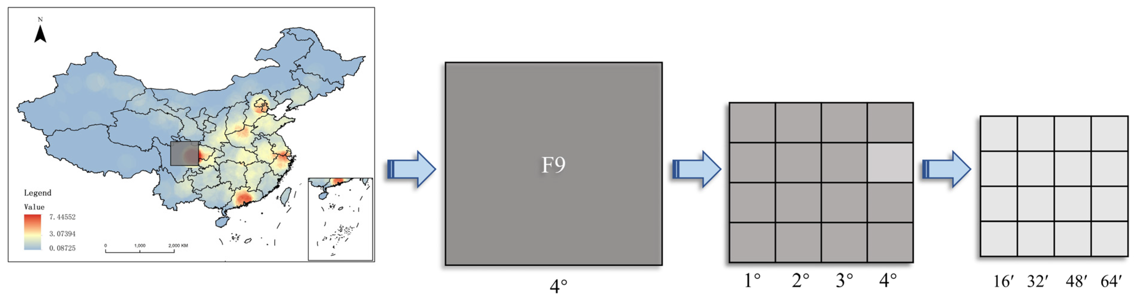
  • The measurable processing of airspace employs spatiotemporal big data technology to re-evaluate airspace use and calculate airspace traffic, thereby providing assistance for further enhancing airspace use efficiency.
  • Calculable decision-making in the airspace by establishing a digital model of the airspace and controlling its operation based on the results of model calculations.

2.1. Visualization Analysis of Airspace

This paper presents a comprehensive and visually processed dataset of all aircraft present at 12:40 (UTC) on a specific day. The dataset includes the aircraft transponder code and the position coordinates in latitude and longitude, velocity, flight altitude, departure airfield, takeoff time, aircraft model, and other parameters. A schematic of the flight route data within the airspace is provided below, along with a visualization analysis of the positional distribution of aircraft operating within the southwestern region of the same airspace. Based on the navigation and monitoring performance and the dynamic division of airspace, the proposed discretization method is helpful for situational awareness under dense traffic conditions, introducing a new and effective 3D airspace visualization scheme and improving the command effect in the tactical stage [23].
Figure 1 below shows the aircraft operating in the airspace at 12:40 (UTC).

2.2. Measurable Processing of Airspace

In this article, the direct discretization method is employed. The function f t can be approximated by a discrete grid function f ( n h ) , where h represents the grid length. Thus, the fractional-order differentiation of this function can be approximated as follows:
y h n h = h r ω δ 1 r f h n h
where δ 1 is the conversion operator, and ω δ 1 is a generating function that determines the form and coefficients of the approximation. Using the sampling time T to replace h and the complex variable Z to replace ω, the function f t can be transformed into the Z-transform of the sequence f ( n h ) , which achieves the discretization approximation of the spatial domain partition.
As the corresponding generating function is an irrational function, a physical and chemical approximation is required. The Tustin algorithm is used to derive the generating function, which is expressed as follows:
ω z 1 ± r = 2 T 1 Z 1 1 + Z 1 ± r
The continued fraction is computationally faster than an exponential sequence. Therefore, using the continued fraction expansion (CFE) of the Tustin operator can provide better approximation results for fractional calculus operators. The continued fraction form of function G is expressed as follows:
G Z = a 0 Z + b 1 Z a 1 Z + b 2 Z a 2 Z + b 3 Z a 3 Z +
When the Tustin operator and CFE method are combined, the discretization model can be approximated as follows, where r [ 1 , 1 ]
D r Z = 1 + Z 1 1 2 1 r + Z 1 2 + Z 1 3 2 r r 2 1 + Z 1 2 + Z 1 5 2 r 2 1 r 4 + r 2 + Z 1 2 +
The discretization description method for metric parameters based on the geodetic coordinate system employs an Earth ellipsoid partitioning method based on the integer rules of longitude and latitude. This involves spatially partitioning the ellipsoid surface into subregions using the integer form of degrees, minutes, and seconds of longitude and latitude. To effectively represent the spatial domain and facilitate the detection of obstacles and restriction zones, a portion of the space is extracted and discretized using continued fraction processing [24]. The further subdivision is carried out at an interval of 1° to form a second-level ellipsoid unit of size 1° starting with an ellipsoid unit of 4° in longitude and latitude. The 1° unit is extended to 64’, further subdivided into subregions of size 16’ to form third-level ellipsoid units. The 16’ regions are then divided into four equal parts, each 4’ in size, until reaching the seventh level, where the unit size reduces to 4″.
Figure 2, below, shows the D(Z) calculated using different fractional-order values of r for spatial partitioning models.
For any spatial region P specified by its latitude–longitude coordinates (B, L), the basic unit for level-one grid partitioning has a spacing of 4° in longitude and latitude, with the reference origin located at the westernmost point of the Pamir plateau in Xinjiang (39°15′ N, 73°33′ W). The level-one spatial unit reference system matrix is denoted by G 13 × 16 1 , and the row/column indices in G 13 × 16 1 corresponding to the level-one grid cell containing point P can be calculated using the following formula:
m = 13 B ° 4 °           n = L ° 4 °
Because the airspace studied is the airspace over a specific region, the longitude and latitude division is concentrated in the region for the first level division (Table 1).
The encoding of the second-level spatial units is carried out by further subdividing a selected space unit from the first-level spatial partitioning using longitude and latitude intervals of 1 degree, with reference to the lower left corner as the origin. For a specified space cell P with longitude and latitude (B, L) and the upper-left corner coordinates of the first-level spatial unit denoted as B 1 , L 1 . The reference grid system matrix for the second level is denoted as G 52 × 64 2 . The following formula can be used to calculate the row and column numbers of the second-level subdivision grid unit containing point P with its longitude and latitude (B, L):
m = B 1 ° 1 °           n = L 1 ° 1 °
To divide the first level, the spatial domain of the first level can be accurately divided by horizontal and vertical signs (Table 2).
The matrix row number m, column number n, and address code M corresponding to the spatial grid unit in the airspace of the partitioning level I can be expressed as follows:
m = b 1 m b 2 m b 6 m b 7 m      n = l 1 n l 2 n l 6 n l 7 n

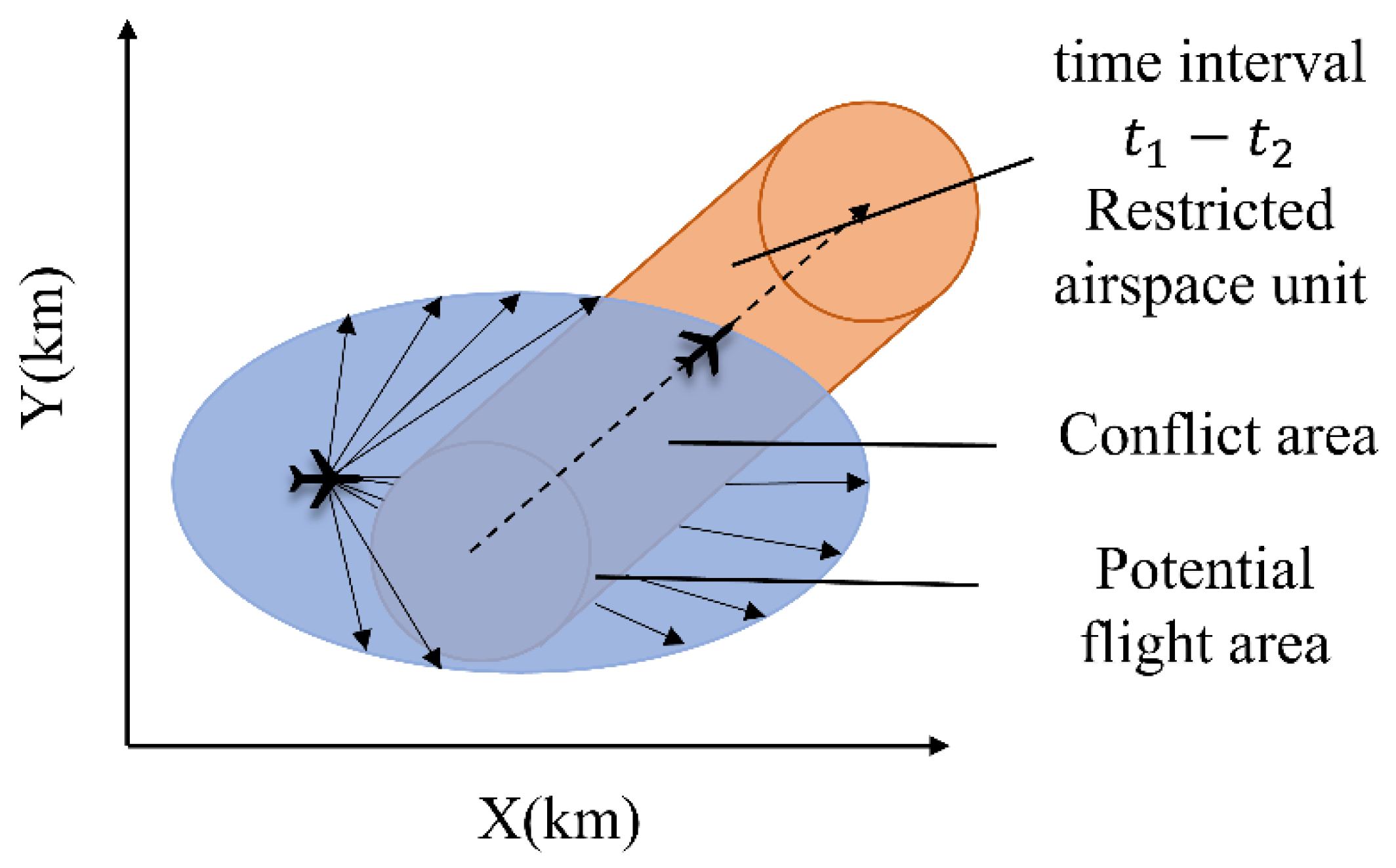
2.3. Calculable Decision-Making in Airspace

The purpose of conflict detection for dynamic flight paths is to investigate the interspersal of the flight trajectory of an aircraft over a period of time with the spatial units occupied by obstacles. Assuming that the time when the aircraft and obstacle collide is t 1 t 2 , the motion trajectory of the aircraft during the time interval t 1 t 2 is characterized, and the trajectory line AOR l i n e B i , i + 1 , L j , j + 1 , t 1,2 is generated.
Figure 3, below, shows the conflict detection status of an aircraft during a period t 1 t 2 .
Vertical layer scope conflict detection is a method used to identify any intersection in the spatial protection zone on the vertical layer. When the vertical layer between an aircraft and an obstacle satisfies the minimum safety interval, the detection of the vertical layer can be skipped, and the horizontal two-dimensional layer can be checked next. Let airspace ‘a’ be a restrictive cell occupied by an obstacle with a height range label of H 1 H 2 , and let airspace ‘b’ be a restrictive cell occupied by the flight path of an aircraft with a height range label of h 1 h 2 . The following cases are considered for conflict judgment between the two airspaces on the vertical layer:
  • h 1 < H 1 < h 2 < H 2 . Partial overlap exists between the vertical layers of the airspace occupied by the obstacle and the flight area of the aircraft;
  • H 1 < h 1 < h 2 < H 2 . The vertical height of the flight area of the aircraft is completely within the vertical height range of the airspace occupied by the obstacle;
  • 0 < H 1 h 1 < Δ h . Even though no intersection exists between the vertical layers of the obstacle and the aircraft, the minimum height of the obstacle’s airspace and the maximum height of the aircraft’s airspace differ by less than ∆h, which represents the minimum safety interval.
In the horizontal level boundary conflict model, the two-dimensional plane shape of the airspace to be detected is characterized in the detection model, revealing whether the boundaries of the detection cells intersect. In a Cartesian coordinate system, assuming that the vertex coordinates of the static flight zone are ( m 1 , n 1 ), ( m 1 , n 2 ), ( m 2 , n 1 ), ( m 2 , n 2 ) and that the vertex coordinates of the obstacle zone are ( m 3 , n 3 ), ( m 3 , n 4 ), ( m 4 , n 3 ), ( m 4 , n 4 ), if m 1 + ∆ m m i m 2 + ∆ m and n 1 + ∆ n n j n 2 + ∆ n , where i , j { 3,4 } , then an overlap is present in the unit templates of the two areas, and a conflict exists. The size of ( m , n ) is determined by the spacing standard between the aircraft and the obstacles.
Figure 4, below, shows the conflict detection model for discretized airspace units of an aircraft.
Based on the discretization method and the different lengths of airspace units divided into different levels represented as D(Z), we propose improved discretization processing steps for aircraft-to-aircraft trajectory planning, as outlined in Algorithm 1:
Algorithm 1: Pseudo-code of the discretization method for airspace planning.
1  Initialize spatial hierarchy element matrix, path, path length, and cost; discrete coding for the airspace occupied by obstacles.
2    repeat
3       for aircraft i = 1 to n do
4         Initialize each aircraft position
5         repeat
6          Each code i + 1 based on calculated risk probability, the probability of using the available cell space, and time resources
7         then clear aircraft i to move to code (m,n); add code (m,n) to the operation path list; and update the aircraft’s position Xi + 1 Xi, path list, time and space cost, and path length
8            end if
9          until the aircraft reaches the destination
10        end for
11        Select the path with the lowest cost
12        repeat
13        if Distance l i n e B i , i + 1 , L j , j + 1 , t 1,2 >=min(SD)
14        then add i,j to the actual airspace operation code set
15        end if
16        If selected, the optimal route of temporal and spatial efficiency differs from the route of the next stage
17         Delete the selected optimal path, select a second optimal path
18        end if
19    until an optimal airspace operation that can meet all the minimum safety distances is selected
20      Update the scenario parameters of different routes in the airspace in the next time period
21  until the number of aircraft N is met
22  Output the optimal airspace code set, then smooth the spatiotemporal efficient optimal airspace operation route of adjacent discrete time points

3. Results

This section expounds on the influence of the discretization method on airspace from two perspectives. The first is the calculation results of flight path planning; the second is the improvement in airspace operation efficiency based on the spatiotemporal efficiency index.

3.1. Evaluation of Airspace Operational Efficiency

By integrating the intrinsic analysis of aircraft operational safety, airspace resource use, and major factors influencing air traffic management, as well as compiling survey results from experts and staff, we identified indicators for evaluating the operating efficiency of airspace systems, as listed below in Table 3.
The above index layer and each index are basically asked by experts and working in the field of controller they pay more attention to the factors affecting the operation of aircraft.
In this study, air traffic controllers who were familiar with the F9 airspace used throughout this study were chosen as the research subjects, and 20 questionnaires were distributed and collected. The Reliability Index of the Questionnaire in F9 airspace is calculated, and the reliability method of test–retest for different test indexes in the software needs to be repeated, which is not feasible. The half-confidence method improves the reliability precision by deducing the theoretical formula, but it is not suitable for the factual questionnaire. The opinion survey was conducted using Cronbach’s alpha reliability coefficient method to ensure the internal consistency of the indicator system using the criteria listed below for verification [25] (Table 4).
From the previous studies on Cronbach’s Alpha Coefficient, the results of the questionnaire index coefficient greater than 0.8, the index is worth considering.
In SPSSAU, the analysis results of each indicator in the airspace operation evaluation index system are summarized below (Table 5).
In this study, Air traffic safety, Airspace operation time, Airspace use rate argets were selected to calculate the efficiency. The results are in the Table A1, Table A2 and Table A3.
As can be seen from the table above, Cronbach’s alpha coefficient (α) of the target layer in the evaluation system designed in this study is above 0.8, indicating high internal consistency among the indicators of the airspace operation evaluation model. The questionnaire survey results show good stability and pass the reliability test.
To comprehensively evaluate the status of airspace operations, the overall evaluation of the airspace must consider the six target layers corresponding to the indicators of airspace operation, namely air traffic safety U 1 , time efficiency U 2 , airspace use rate U 3 , airspace flexibility U 4 , operational effectiveness U 5 , and cost efficiency U 6 in the overall layer. An evaluation index matrix is constructed for each indicator within each target layer as follows: the air traffic safety index matrix U 1 = U 11 , U 12 , U 13 , U 14 20 , the airspace time efficiency index matrix U 2 = U 21 , U 22 , U 23 , U 24 , U 25 , U 26 20 , the airspace use rate index matrix U 3 = U 31 , U 32 , U 33 , U 34 , U 35 20 , the airspace flexibility index matrix U 4 = U 41 , U 42 , U 43 20 , the operational effectiveness index matrix U 5 = U 51 , U 52 , U 53 20 , and the cost-efficiency index matrix U 6 = U 61 , U 62 , U 63 , U 64 , U 65 20 .
In the evaluation of airspace operational efficiency, all the indicators adopted are inverse indicators. When the value of the indicator p i is close to 0, the overall spatial and temporal efficiency of the airspace is high, and when the value is close to 1, the airspace’s temporal and spatial efficiency is low. This principle guides the evaluation process.
Figure 5, below, shows the a schematic diagram of the operational efficiency of airspace is evaluated by the extension analytic hierarchy process.
Let p * = p 1 * , p 2 * p i * T , p * * = p 1 * * , p 2 * * p i * * T , and p * * * = p 1 * * * , p 2 * * * , p i * * * T be the level thresholds corresponding to the i indicator. The thresholds for each level of the indicators are satisfied.
i = 1 n p i * 2 = r * 2 , i = 1 n p i * * 2 = r * * 2 , i = 1 n p i * * * 2 = r * * * 2
With the weight vectors obtained through the analytic hierarchy process, the judgment of the airspace operational efficiency evaluation thresholds can be expressed as f # = r # . Evaluations are based on the value of the threshold matrices, and all the units p i are computed. The evaluation threshold matrix for “excellent” and “good” airspace operational efficiency levels is defined as ( p 1 * , p 2 * , p 3 * , p i * ) , with the value of the judgment taken as the 10th percentile of the total number of airspace units. The boundary point between the “good” and “fair” aviation efficiency levels is identified by the value of the judgment taken as the 25th percentile of the total number of airspace units. This corresponds to an evaluation threshold matrix defined as ( p 1 * * , p 2 * * , p 3 * * , p i * * ) . The boundary point between the “fair” and “poor” aviation efficiency levels is set by the value of the judgment taken as the 40th percentile of the total number of airspace units. This denotes an evaluation threshold matrix defined as ( p 1 * * * , p 2 * * * , p 3 * * * , p i * * * ) . The thresholds p i * , p i * * , and p i * * * are determined in accordance with the thresholds of airspace operational efficiency.
Using the comprehensive assessment model established for airspace operational efficiency, specific indicator values are computed, and the value of each time–space efficiency indicator is standardized to a range of 0 to 1. The comprehensive airspace operational efficiency f U s t is evaluated using a comprehensive evaluation function.
The thresholds of different levels are calculated, and the evaluation level of the operational efficiency of airspace is judged (Table 6).
This paper used the extreme value method to preprocess the indicators by determining the minimum and maximum values of each indicator to ensure that all indicator values are between 0 and 1. Let M j = m a x x i j and m j = m i n x i j , where x i j is the value corresponding to the j indicator. According to the extreme value method, the normalized value x j # = x j m j / M j m j . The modified matrix for the evaluation thresholds of airspace operational efficiency, combining this with the evaluation matrix, can be obtained as U 1 # , U 2 # ,   U 3 # ,   U 4 # ,   U 5 # ,   U 6 # .
Next, using the identified targets and indicators, the weights of the indicators are determined by applying the AHP analysis method to judge the relative importance of each target and indicator. By constructing an extended interval number judgment matrix according to the 20 returned questionnaires, the extension interval number of target layer i and index layer j was obtained, a i j k = a i j 1 + a i j 2 + a i j 20 / 20 , and based on the degree of superiority or inferiority of each target and indicator, the comprehensive extended interval number matrix, A = A , A + , was obtained. The comprehensive extended interval weight vector α = φ x , μ x + = a 1 , a 2 , a 20 T that satisfies the consistency condition φ ,   μ is calculated using the following formula:
φ = j = 1 n 1 1 n A , μ = j = 1 n 1 1 n A +
Here, the weight vector P i k = S i k , S i k + 2 = P 1 i k , P 2 i k P n i k 20 is then obtained for the kth layer with respect to the previous target layer, where S k = S 1 k , S 2 k , S n k 20 = φ x , μ x + and P i k represents the weight vector of the i target layer.
The target layers for airspace operations using the extended analytic hierarchy process method to determine weight vectors are represented as U 1 = u 11 , u 12 u 1 n , U 2 = u 21 , u 22 u 2 n , and U n = u n 1 , u n 2 u n n , and the vector for the overall layer of airspace operational efficiency with respect to the target layers is represented as U = U 1 , U 2 , U n .
The evaluation and analysis of the indicators were conducted for a certain period in the Southwest China airspace. The threshold values for each indicator satisfied the following formula:
i = 1 n u i j * 2 = r * 2 , i = 1 n u i j * * 2 = r * * 2 , i = 1 n u i j * * * 2 = r * * * 2
The index values of each target layer were obtained through 20 questionnaires, and the values of each index are illustrated in the Appendix A.
For the overall layer of operational efficiency, using the weight vector obtained from the calculation combined with the operational evaluation function, the comprehensive evaluation function of airspace operation efficiency could be calculated as f # = U 1 · U 1 * · U 1 * T , U 2 · U 2 * · U 2 * T , U n · U n * · U n * T = r # . By evaluating each target layer, the thresholds listed below were obtained.
In Table 7, when evaluating the operational efficiency of airspace by extension layer method, the indexes are all inverse indexes, and the index efficiency is high when the value is close to 0, and low when the value is close to 1.
The comprehensive operational efficiency of airspace before and after discretization was evaluated using the extenics-based comprehensive evaluation function, expressed as f = U 1 · U 1 # · U 1 # T , U 2 · U 2 # · U 2 # T , U n · U n # · U n # T = r 2 . The evaluation thresholds determined for different levels are listed below (Table 8).
The operational efficiency of the airspace using the evaluation function was calculated as f # = U 1 · U 1 * · U 1 * T , U 2 · U 2 * · U 2 * T , U n · U n * · U n * T = 0.03173 . Upon comparing with the judgment thresholds, we determined that the airspace’s operational efficiency was “medium”.

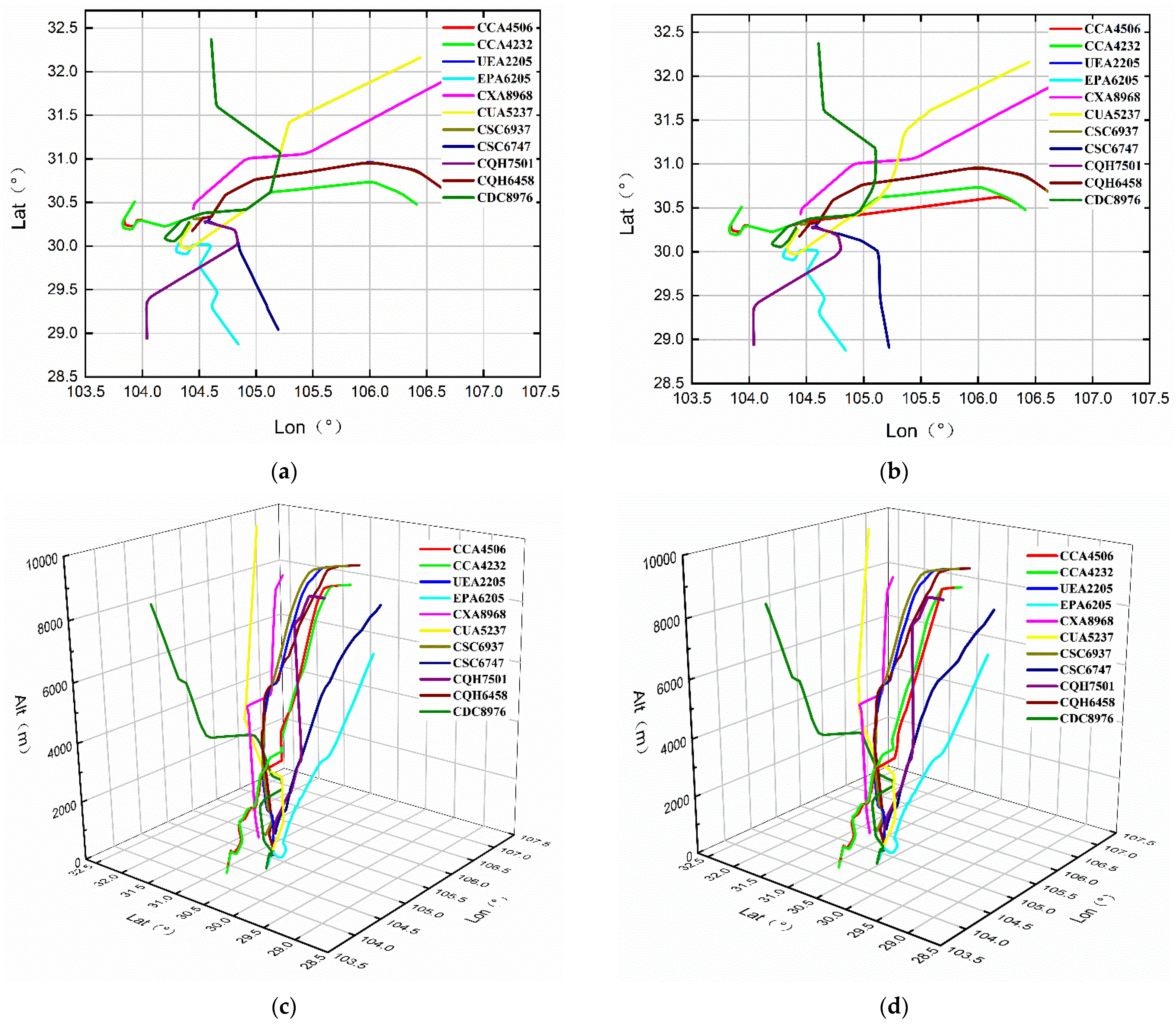
3.2. Improvement of Operation Efficiency by Discretization

3.2.1. Safe Interval

Safety assessment considerations for aircraft include flight paths and aircraft feasible regions. The set of all feasible positions constitutes the feasible region of the aircraft’s R i   F D i t [26], which is represented as follows:
F D i t = W O b s j
where F D i t is the available grid of aircraft R i at time t; W is the set of all points in the work area location P k , P l W ; and P l does not exist in the grid of obstacles or limits O b s j , so that P l is aircraft R i ’s feasible region F P i t .
Different provisions are set for the horizontal and vertical spacing of various aircraft types or in diverse weather conditions for the airspace between flight routes. Uniformly stipulated as S s , these requirements specify, for instance, that the vertical spacing between two aircraft should be no less than 300 m and the horizontal distance should be no less than 10 km. Consequently, the minimum safety separation for the rerouted flight path must meet the following requirements:
m i n S x , y , d S s , d W
By studying the relationship between airspace planning and UAV paths, the Cartesian path discretization method for UAVs and the new 4D path discretization method were compared, and the advantages of the algorithm were determined [27]. The discretization of protected and available cells at different levels was carried out in the obstacle avoidance area between the aircraft and obstacles, and the resulting turning path was smoothed, as shown below.
Figure 6 below shows the aircraft operating in the airspace at 12:40 (UTC).

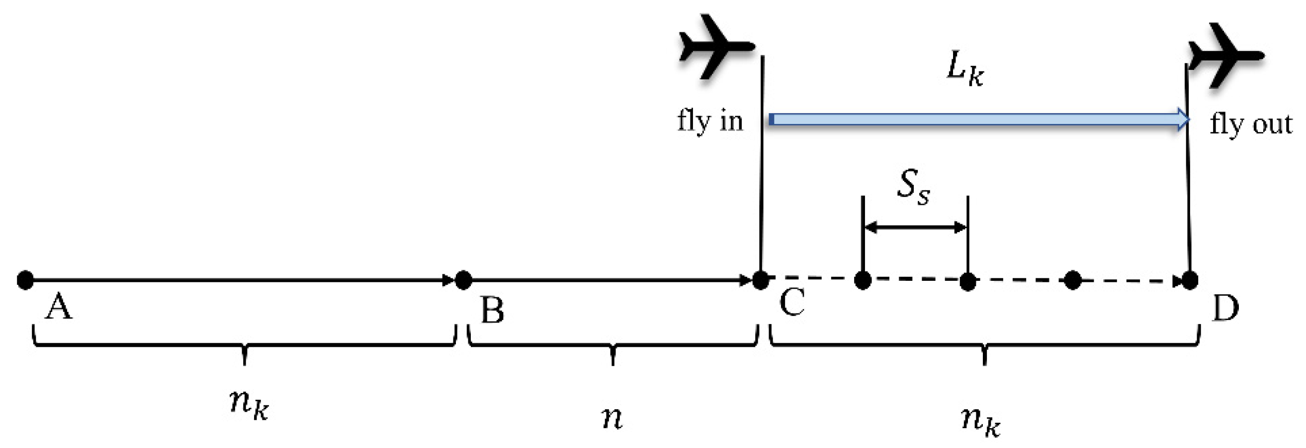
3.2.2. Time Efficiency

The time efficiency index of airspace can be defined as the ratio between the sum of the actual flight crossing times of aircraft flying over an airspace within a specific time and the sum of all available flight crossing times for flights determined by the airspace capacity of that airspace. This index quantifies airspace use within a given period and provides insights into the effectiveness of flight planning strategies in managing airspace resources. The formula is as follows:
U = T r T t × 100 %
where U represents the spatiotemporal efficiency of the airspace, T r denotes the total flight time for aircraft flying over airspace within a specific period, and T t represents the total available flight time for all aircraft that can use the airspace.
Figure 7, below, shows the maximum number of aircraft considered as particles in a airspace.
The formula for the total duration T k m a of the actual flight passage of aircraft in the airspace is as follows:
T k m a = j = 1 n m T k m j
where n m refers to the number of aircraft flying at different altitudes, and T k m j represents the total flight crossing time for aircraft j spanning from its entry into the airspace until its exit.
Each aircraft within the airspace is considered a point mass, and when the traffic volume along the flight route in the airspace approaches its maximum capacity of n k , the formula for calculating the airspace capacity is as follows:
n k = L k S s
where L k is the length of route k, and S s refers to the minimum safety interval to be maintained between aircraft, which is m i n S x , y , d S s .
At the end of a specified period t, an aircraft is located precisely at position C. The average speed of the aircraft is V k ¯ , and its average flight track length is t j ¯ ; thus, the distance covered by the aircraft during period t, from A to C, can be computed as L A C = V k ¯ · t . The total number of aircraft within segment AC can be determined using the following formula:
n k + n = L A C / S s = V k ¯ · t / S s
where n k is the number of aircraft that have flown into the entry point but not out of the exit, n refers to the number of aircraft that have flown out of the exit before the time is up, and L A C indicates the length of two segments of AC, and the average speed of the aircraft is V k ¯ .
The formula for the number of aircraft in segment BC is as follows:
n = L B C / S s n k
AB and CD are the routes of any two aircraft flying over the airspace during this period for t k ¯ , and AB and CD are the routes of two aircraft in the airspace during the whole period for n k · t k ¯ . For a certain period, the theoretical maximum total flight time T k m t of this airspace route is calculated as follows:
T k m t = n k · t k ¯ + n · t k ¯ = L k S s + V k ¯ · t L k S s · t k ¯ = V k ¯ · t S s · t k ¯
The calculation model for the time efficiency of flying over certain airspace is as follows:
U k m = T k m a T k m t = j = 1 n m t k m j V k ¯ · t S s · t k ¯

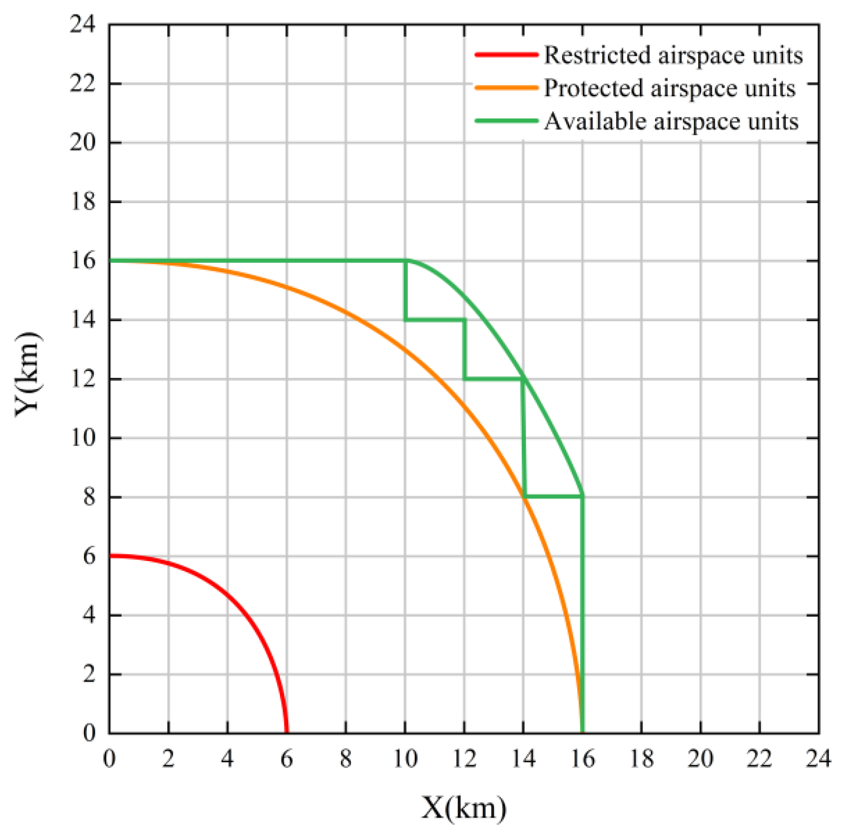
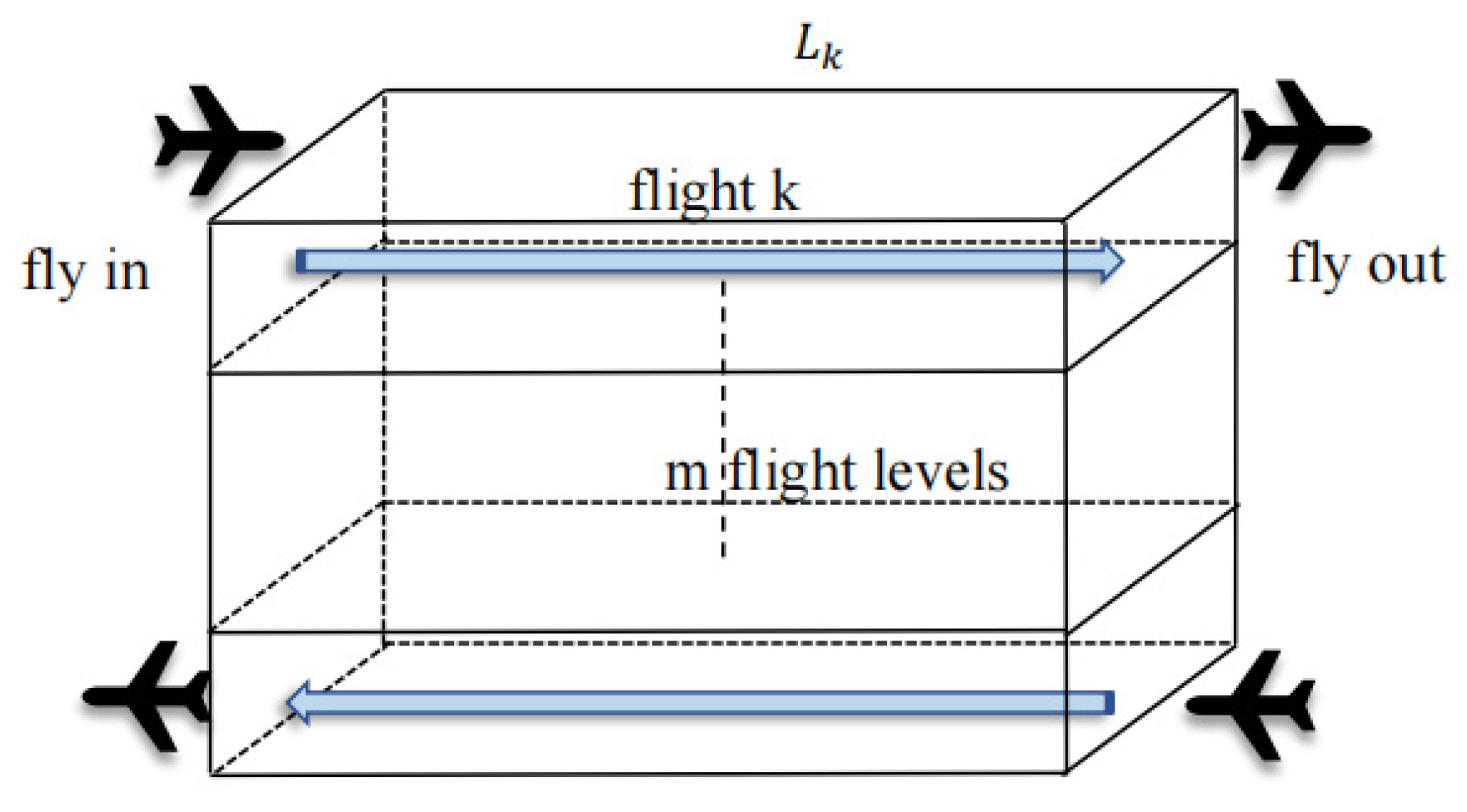
3.2.3. Space Efficiency

According to the definition of the use rate of the altitude layer, an aircraft is considered a particle, and the maximum number of aircraft accommodated by the altitude layer is calculated by the aircraft velocity and the length of the route in the altitude layer.
Figure 8 below shows the flight status at different flight levels.
The total number of aircraft and the number of aircraft accommodated in route k are calculated from the historical data of the airspace. Then, the use rate of route k is calculated as follows:
U k = k P k m U k m
where U k is the use rate of route k and P k m is the probability of an aircraft appearing during a certain period.
The operation conditions of each altitude layer in airspace differ. In order to accurately calculate the space use rate of airspace, it is necessary to determine the occurrence probability of aircraft flow at each altitude layer in the airspace, sum the use rate of each altitude layer, and obtain the space use rate of the whole airspace at a certain time, as follows:
U ε = k U k = k m P k m U k m
The F9 airspace was discretized, and the flight path of an aircraft in the congested airspace at 12:40 UTC was visualized. The flight path was planned by discretization so that it conformed to the optimal time efficiency and space use rate of the airspace.
Figure 9, below, displays information pertaining to aircraft operating in heavily congested airspace; all available flight path and optimized flight path data for aircraft operating within the airspace at 12:40 (UTC) were acquired.
The extenics-based analytic hierarchy process was used to determine the weight vectors. In the third level, the three weighted vector indicators for airspace time efficiency, airspace spatial use efficiency, and safety were evaluated as A 1 = a 1 , a 2 a n , B 1 = b 1 , b 2 b n , and C 1 = c 1 , c 2 c n , respectively. The vector A = A 1 , B 1 , C 1 represents the overall airspace operational efficiency with respect to the target layer.
A comprehensive extenics judgment matrix was established for the effectiveness of airspace operation in terms of spatiotemporal efficiency based on the three target layers of air traffic safety, time efficiency, and spatial use efficiency (Table 9).
The normalized characteristic vectors of A , A + were calculated as follows:
A = 1 0.18 0.37 3.75 1 3.5 2.1 0.27 1 , A + = 1 0.27 0.48 5.56 1 3.7 2.7 0.29 1
The normalized eigenvectors of A , A + were calculated as follows:
x = 0.111 , 0.663 , 0.226 , x + = 0.122 , 0.653 , 0.225
The weight vector of the extenics interval numbers was calculated as follows:
ω = φ x , μ x + = 0.108 0.643 0.22 0.125 0.666 0.229 20
By evaluating the indicators in the target layer individually, we obtained A 1 = a 1 , a 2 a n = (0.117, 0.236, 0.276, 0.303), B 1 = b 1 , b 2 b n   = (0.211, 0.208, 0.281, 0.224, 0.197, 0.264), a n d   C 1 = c 1 , c 2 c n = (0.432, 0.468, 0.481, 0.458, 0.464).
By incorporating the indicators of air traffic safety, time efficiency, and spatial use efficiency into the comprehensive evaluation function, the operational efficiency of the airspace, f # = A 1 · A 1 * · A 1 * T , B 2 · B 2 * · B 2 * T ,   C 3 · C 3 * · C 3 * T = 0.02168 , was obtained. From the range r * f # r * * , we could conclude that the airspace operation efficiency was “good”. The entire evaluation process and results indicated that improving the indicators of air traffic safety, time efficiency, and spatial use efficiency through discretization will enhance the operational efficiency of airspace.

4. Conclusions

After compiling data on the operational status of airspace, a method for discretizing the airspace was employed, considering metrics such as time efficiency, air traffic safety, and airspace use rates to optimize flight paths. The overall efficiency of the airspace operation was assessed using the extension analysis method, with an efficiency threshold of 0.02168. The result was “good”, representing a significant improvement over the original efficiency score of 0.03173.
The innovative contributions of this research project are as follows:
(1)
A novel spatial discretization method suited for local airspace was proposed that can precisely represent any given airspace cell in three-dimensional space. This discretization method makes visualizing airspace use much easier, providing a theoretical foundation for air traffic controllers to guide aircraft more accurately as they alter their flight paths.
(2)
A new model was developed for evaluating the operational efficiency of airspace based on discretized data, focusing on three key elements, time efficiency, air traffic safety management, and airspace use. By combining the weighting of different indicators within the overall airspace performance layer, the model is capable of quantifying airspace operational performance more effectively.
(3)
Improvements were made to enhance operational efficiency within a specific airspace. The algorithm developed here uses multiple discrete trajectory planning techniques for corresponding flight paths, enabling air traffic controllers to guide flights through highly congested environments more efficiently while increasing overall airspace performance efficiency.
In summary, this study provides a practical approach to improving operational efficiency within heavily trafficked airspace while ensuring the highest levels of safety.

Author Contributions

Supervision, D.Z.; writing—original draft preparation, Z.C.; software, X.X.; validation, J.C.; data curation, Z.C.; funding acquisition, D.Z. All authors have read and agreed to the published version of the manuscript.

Funding

This research was funded by the Civil Aviation Safety Capacity Building Project of China (grant number 14002600100015J013).

Data Availability Statement

The original data are not publicly available but can be used for scientific research. Researchers should email the first author if needed.

Conflicts of Interest

The authors declare no conflict of interest.

Appendix A. Index Survey

The following normalized indicators all have values between 0 and 1. The closer an indicator’s value is to 1, the better the evaluation result. Conversely, the closer an indicator’s value is to 0, the worse the evaluation result.
Table A1. Investigation of airspace operation safety index recognition degree.
IndicatorIndicator ValueThresholdCorresponding GradeEvaluationNormalization
Number of Conflicts0[0–0.1)ExcellentExcellent0
[0.1–0.5)Good
[0.5–0.9)Medium
[0.9–1)Poor
Potential Conflict Alert Time70[0–46)ExcellentGood0.316
[46–128)Good
[128–225)Medium
[225–415)Poor
Potential Conflict
Minimum Distance
8.87[42–48)ExcellentMedium0.364
[24–42)Good
[8–24)Medium
[0–8)Poor
Safety
Management Level
0.56[0.9–1)ExcellentGood0.31
[0.6–0.9)Good
[0.1–0.6)Medium
[0–0.1)Poor
Table A2. Investigation of airspace operation time index recognition degree.
IndicatorIndicator ValueThresholdCorresponding GradeEvaluationNormalization
Restricted Airspace Use Time0.027[0–0.1)ExcellentExcellent0.13
[0.1–0.5)Good
[0.5–0.9)Medium
[0.9–1)Poor
Peak Hour Delay766[0–206)ExcellentMedium0.443
[206–688)Good
[688–1114)Medium
[1114–1724)Poor
Average Arrival Delay548[0–206)ExcellentGood0.374
[206–688)Good
[688–1114)Medium
[1114–1724)Poor
Average Departure Delay461[0–206)ExcellentGood0.336
[206–688)Good
[688–1114)Medium
[1114–1724)Poor
Airspace Time Use Capability0.56[0.9–1)ExcellentMedium0.324
[0.6–0.9)Good
[0.2–0.6)Medium
[0–0.2)Poor
Table A3. Investigation of airspace use rate index recognition degree.
IndicatorIndicator ValueThresholdCorresponding GradeEvaluationNormalization
Route Use Rate0.191[0–0.1)ExcellentGood0.236
[0.1–0.5)Good
[0.5–0.9)Medium
[0.9–1)Poor
Airspace Spatial Use Capability11[15–17)ExcellentMedium0.341
[12–15)Good
[9–13)Medium
[5–9)Poor
Airspace Route Network Connectivity80[90–100)ExcellentGood0.275
[75–90)Good
[60–75)Medium
[0–60)Poor
Airspace Sector Saturation0.869[0.9–1)ExcellentGood0.283
[0.6–0.9)Good
[0.1–0.6)Medium
[0–0.1)Poor
Airport Approach and Departure Capacity0.613[0.8–1)ExcellentGood0.268
[0.6–0.8)Good
[0.2–0.6)Medium
[0–0.2)Poor
The three appendices show the numerical values and judging criteria of each index threshold of the three important target layers in the evaluation of airspace operational efficiency.

References

  1. Ye, K.P. Maintenance and accuracy analysis of regional reference frame based on reference station network. Mapp. Spat. Geogr. Inf. 2019, 42, 148–150+154. [Google Scholar]
  2. Zhang, X.G.; Lv, Z.P. On Maintenance of the Earth Frame of Reference. Bull. Surv. Mapp. Beijing 2009, 5, 1–4. [Google Scholar]
  3. Tong, X.; Ben, J.; Wang, Y.; Zhang, Y.; Pei, T. Efficient encoding and spatial operation scheme for aperture 4 hexagonal discrete global grid system. Int. J. Geogr. Inf. Sci. 2013, 27, 898–921. [Google Scholar] [CrossRef]
  4. Wambsganss, M.C. GPS outage impacts on the national airspace system. In Proceedings of the 2013 Aviation Technology, Integration, and Operations Conference, Los Angeles, CA, USA, 12–14 August 2013. [Google Scholar]
  5. Stankūnas, J.; Kondroška, V. Formation of methodology to model regional airspace with reference to traffic flows. Aviation 2012, 16, 69–75. [Google Scholar] [CrossRef]
  6. Kondroška, V.; Stankūnas, J. Analysis of airspace organization considering air traffic flows. Transport 2012, 27, 219–228. [Google Scholar] [CrossRef]
  7. Kaplan, C.; Dahm, J.; Oran, E.; Alexandrov, N.; Boris, J. Analysis of the monotonic Lagrangian grid as an air traffic simulation tool. J. Guid. Control Dyn. 2013, 36, 196–206. [Google Scholar] [CrossRef]
  8. An, J.X.; Wang, W.X.; Liu, Z.; Zhang, J.Q. A route planning method based on the airspace divided by grid method. Proc. Adv. Mater. Res. 2015, 1073–1076, 2381–2384. [Google Scholar] [CrossRef]
  9. Wang, S.; Li, Q.; Cao, X.; Li, H. Optimization of air route network nodes to avoid ‘three areas’ based on an adaptive ant colony algorithm. Trans. Nanjing Univ. Aeronaut. Astronaut. 2016, 33, 469–478. [Google Scholar]
  10. Matthews, B.; Nielsen, D.; Schade, J.; Chan, K.; Kiniry, M. Comparative study of metroplex airspace and procedures using machine learning to discover flight track anomalies. In Proceedings of the 2015 IEEE/AIAA 34th Digital Avionics Systems Conference (DASC), Prague, Czech Republic, 13–17 September 2015. [Google Scholar]
  11. Sergeeva, M.; Delahaye, D.; Mancel, C.; Vidosavljevic, A. Dynamic airspace configuration by genetic algorithm. J. Traffic Transp. Eng. Engl. Ed. 2017, 4, 300–314. [Google Scholar] [CrossRef]
  12. Gerdes, I.; Temme, A.; Schultz, M. Dynamic airspace sectorisation for flight-centric operations. Transp. Res. Pt. C-Emerg. Technol. 2018, 95, 460–480. [Google Scholar] [CrossRef]
  13. Gerdes, I.; Temme, A.; Schultz, M. From free-route air traffic to an adapted dynamic main-flow system. Transp. Res. Pt. C-Emerg. Technol. 2020, 115, 102633. [Google Scholar] [CrossRef]
  14. Yang, S.; He, Z.; Chen, Y.-P.P. GCOTraj: A storage approach for historical trajectory data sets using grid cells ordering. Inf. Sci. 2018, 459, 1–19. [Google Scholar] [CrossRef]
  15. Alam, S.; Chaimatanan, S.; Delahaye, D.; Feron, E. Metaheuristic Approach for Distributed Trajectory Planning for European Functional Airspace Blocks. J. Air Transp. 2018, 26, 81–93. [Google Scholar] [CrossRef]
  16. Zhang, J.; Zhang, P.; Li, Z.; Zou, X. A sector capacity assessment method based on airspace utilization efficiency. Proc. J. Phys. Conf. Ser. 2018, 976, 012014. [Google Scholar] [CrossRef]
  17. Wang, Z.; Zhang, H.; Hu, M.; Qiu, Q.; Liu, H. Analysis of safety characteristics of flight situation in complex low-altitude airspace. Adv. Mech. Eng. 2018, 10, 1687814018774656. [Google Scholar] [CrossRef]
  18. Miao, S.; Cheng, C.; Zhai, W. A low-altitude flight conflict detection algorithm based on a multilevel grid spatiotemporal index. ISPRS Int. J. Geo-Inf. 2019, 8, 289. [Google Scholar] [CrossRef]
  19. Zhu, Y.W.; Chen, Z.J.; Pu, F.; Wang, J.L. Research on the development of digital airspace system. Chin. Eng. Sci. 2021, 23, 135–143. [Google Scholar] [CrossRef]
  20. Chen, Y.T.; Hu, M.H.; Yu, L. Autonomous planning of optimal four-dimensional trajectory for real-time en-route airspace operation with solution space visualisation. Transp. Res. Part C 2022, 140, 103701. [Google Scholar] [CrossRef]
  21. Tluchor, T.; Kleczatsky, A.; Kraus, J. Division of VLL into Specific Airspaces for UAS Operation. In Proceedings of the 23rd International Scientific Conference on New Trends in Civil Aviation (NTCA), Prague, Czech Republic, 26–27 October 2022; pp. 171–176. [Google Scholar]
  22. Babel, L. Coordinated flight path planning for a fleet of missiles in high-risk areas. Robotica 2023, 41, 1568–1589. [Google Scholar] [CrossRef]
  23. Pongsakornsathien, N.; Bijjahalli, S.; Gardi, A.; Sabatini, R.; Kistan, T. A Novel Navigation Performance-based Airspace Model for Urban Air Mobility. In Proceedings of the 2020 AIAA/IEEE 39th Digital Avionics Systems Conference (DASC), San Antonio, TX, USA, 11–15 October 2020; pp. 1–6. [Google Scholar] [CrossRef]
  24. Zhu, Y.W.; Pu, F. Principle and application of spatial grid identification in airspace. Trans. Beijing Univ. Aeronaut. Astronaut. 2021, 47, 2462–2474. [Google Scholar]
  25. Bujang, M.A.; Omar, E.D.; Baharum, N.A. A review on sample size determination for Cronbach’s alpha test: A simple guide for researchers. Malays. J. Med. Sci. MJMS 2018, 25, 85. [Google Scholar] [CrossRef] [PubMed]
  26. Abin, A.A.; Nabavi, S.; Moghaddam, M.E. Using social media for flight path safety assessment. Aircr. Eng. Aerosp. Technol. 2021, 93, 1664–1673. [Google Scholar] [CrossRef]
  27. ElSayed, M.; Mohamed, M. The Impact of Airspace Discretization on the Energy Consumption of Autonomous Unmanned Aerial Vehicles (Drones). Energies 2022, 15, 5074. [Google Scholar] [CrossRef]
Figure 1. The operational status of airborne vehicles in the airspace at 12:40. Within this airspace unit, the maximum number of aircraft reached 7.44552, which means the average number of aircraft in second-level airspace units. The calculated value is not an integer because it is too complicated to determine the position of the aircraft when it appears on the edge line of the airspace unit, so it is calculated by the ratio of the total number of aircraft to the number of airspace units. Further investigation revealed that the airspace of Southwest China was densely populated with aircraft, resulting in congestion. As a case study, this article applies discretization techniques to the airspace unit presented above.
Aerospace 10 00780 g001
Figure 2. The discretization method divides the airspace of the F9 airspace unit into different levels, thus gradually and accurately determining the position of the aircraft, a metric processing schematic for the airspace in which aircraft positions are determined step by step.
Aerospace 10 00780 g002
Figure 3. The potential path region is the projection of the potential motion space-time domain on the plane, which represents the set of all the space positions that the aircraft can reach under a period of time constraint. The potential path region is an ellipse that focuses on the starting and ending waypoints.
Aerospace 10 00780 g003
Figure 4. An aircraft’s collision detection process for boundary units or obstacles: (a) no boundary conflict, (b) no boundary conflict but minimum safe distance not met, (c) boundary unit conflict, and (d) aircraft collides with another aircraft or obstacle.
Aerospace 10 00780 g004
Figure 5. According to the principle of the state classification and evaluation method, different levels of evaluation thresholds are obtained according to each index ( p * , p * * , p * * * , p * * * * ).
Aerospace 10 00780 g005
Figure 6. The obstacle shown in the figure occupies a space cell of 6, the protected area of the obstacle is a horizontal interval of 10 km, and the boundary of the tangent and restricted cells is for the available space cell because the aircraft track is as smooth a curve as possible, the aircraft can be smoothed using units.
Aerospace 10 00780 g006
Figure 7. The aircraft time efficiency calculation for a section of airspace.
Aerospace 10 00780 g007
Figure 8. The figure shows a section of airspace m altitude level of the air routes, each of which has k aircraft.
Aerospace 10 00780 g008
Figure 9. Part of the three-dimensional position data of 6 departing flights and five approaching flights in an airspace unit. The two-dimensional and three-dimensional flight paths of 11 aircraft during this period are shown in graphs (a) and (c). The congestion degree of the discrete airspace cells used by the aircraft was analyzed, and the flight paths of the aircraft covered by the airspace with low operating efficiency were optimized. According to expert opinion, the flight path of the aircraft was not easy to change, so the flight path of the approaching aircraft was optimized based on the restrictions of time, space use rate, and air traffic safety. After the occupied airspace was discretized, the data for the new flight path of the aircraft in this airspace are shown in figures (b) and (d).
Aerospace 10 00780 g009
Table 1. The semantic interpretation of the alphabetic coding for level-one grid units.
LevelLine
Number
Latitude
Interval (°)
Level
Number
Column
Number
Longitude
Interval (°)
A1 B [ 54 ,   50 ) 11 L [ 72 ,   76 )
B2 B [ 50 ,   46 ) 22 L [ 76 ,   80 )
C3 B [ 46 ,   42 ) 33 L [ 80 ,   84 )
D4 B [ 42 ,   38 ) 44 L [ 84 ,   88 )
E5 B [ 38 ,   34 ) 55 L [ 88 ,   92 )
F6 B [ 34 ,   30 ) 66 L [ 92 ,   96 )
G7 B [ 30 ,   26 ) 77 L [ 96 ,   100 )
H8 B [ 26 ,   22 ) 88 L [ 100 ,   104 )
I9 B [ 22 ,   18 ) 99 L [ 104 ,   108 )
J10 B [ 18 ,   14 ) 1010 L [ 108 ,   112 )
K11 B [ 14 ,   10 ) 1111 L [ 112 ,   116 )
L12 B [ 10 ,   6 ) 1212 L [ 116 ,   120 )
M13 B [ 6 ,   2 ) 1313 L [ 120 ,   124 )
1414 L [ 124 ,   128 )
1515 L [ 128 ,   132 )
1616 L [ 132 ,   136 )
Table 2. The semantic interpretation of the alphabetic coding for level-two grid units.
LevelLine
Number
Latitude
Interval (°)
Level
Number
Column
Number
Longitude
Interval (°)
A1 B [ 0 ,   1 ) 11 L [ 0 ,   1 )
B2 B [ 1 ,   2 ) 22 L [ 1 ,   2 )
C3 B [ 2 ,   3 ) 33 L [ 2 ,   3 )
D4 B [ 3 ,   4 ) 44 L [ 3 ,   4 )
Table 3. Evaluation indicators for airspace operational efficiency.
Overall LevelObjective LevelIndicator
Airspace system operating efficiency evaluation indicatorsAir traffic safety U 1 Number of conflicts U 11 , potential conflict alert time U 12 , potential conflict minimum distance U 13 , safety management level U 14
Airspace operation time U 2 Average delay time U 21 , peak hour delay U 22 , average arrival delay time U 23 , average departure delay time U 24 , restricted airspace use time U 25 , airspace time use capability U 26
Airspace use rate U 3 Route use rate U 31 , airspace spatial use capability U 32 , airspace route network connectivity U 33 , airspace sector saturation U 34 , airport approach and departure capacity U 35
Operational flexibility U 4 Temporary flight adjustment capability U 41 , number of flights changing altitude U 42 , number of flights changing routes U 43
Operational effectiveness U 5 Aircraft’s normal clearance rate U 51 , system equipment support capability U 52 , non-linear coefficient U 53
Cost efficiency U 6 Cost conversion capability U 61 , personnel use efficiency U 62 , fuel consumption U 63 , personnel workload U 64 , delay cost U 65
Table 4. Reliability verification standards.
Cronbach s   Alpha   Coefficient   ( α ) Internal Consistency of Indicators
α > 0.9 High
0.9 > α > 0.8 Acceptable
0.8 > α > 0.7 Some indicators are not reasonable, but still useful
0.7 > α > 0.6 Should be reconsidered
Table 5. Approval of airspace operational efficiency indicators.
Airspace Operational Efficiency IndicatorApproval Degree Cronbach s   Alpha   Coefficient   ( α )
Air traffic safety U 1 0.845 α = 0.901
Airspace operation time U 2 0.883
Airspace use rate U 3 0.781
Operational flexibility U 4 0.770
Operational effectiveness U 5 0.725
Cost efficiency U 6 0.671
Table 6. Numerical judgment results of operational efficiency evaluation.
Operational Efficiency ValueAssessment Result
f r * Excellent
r * f r * * Good
r * * f r * * * Medium
f r * * * Poor
Table 7. Evaluation index thresholds.
Operational Efficiency Target Layer m j P * P * * P * * * P * * * * M j
U 1 00.3000.3100.3600.4301
U 2 00.2700.2900.3220.3971
U 3 00.2560.2780.3110.3571
U 4 00.1700.1970.2030.2581
U 5 00.1700.2050.2110.2691
U 6 00.0870.0940.1050.1121
Table 8. Comprehensive evaluation index thresholds.
Judgment Threshold r * r * * r * * * r * * * *
Threshold Value0.016790.023790.039070.06475
Judgment Threshold f   * f   * * f   * * * f   * * * *
Threshold Value0.0002820.0005660.0015260.004193
Table 9. The judgment matrix for the number of extension intervals between the overall layer and the target layer.
Overall LevelObjective Level
Safe IntervalTime EfficiencySpace Efficiency
Safe Interval(1, 1)(0.18, 0.27)(0.37, 0.48)
Time Efficiency(3.75, 5.56)(1, 1)(3.5, 3.7)
Space Efficiency(2.1, 2.7)(0.27, 0.29)(1, 1)
Disclaimer/Publisher’s Note: The statements, opinions and data contained in all publications are solely those of the individual author(s) and contributor(s) and not of MDPI and/or the editor(s). MDPI and/or the editor(s) disclaim responsibility for any injury to people or property resulting from any ideas, methods, instructions or products referred to in the content.

