Abstract
Minimizing electric losses is critical to the success of battery-powered small unmanned aerial systems (SUASs) that weigh less than 25 kgf (55 lb). Losses increase energy and battery weight requirements which hinder the vehicle’s range and endurance. However, engineers do not have appropriate models to estimate the losses of a motor, motor controller, or battery. The aerospace literature often assumes an ideal electrical efficiency or describes modeling approaches that are more suitable for controls engineers. The electrical literature describes detailed design tools that target the motor designer. We developed SUAS powertrain models targeted for vehicle designers and systems engineers. The analytical models predict each component’s losses using high-level specifications readily published in SUAS component datasheets. We validated the models against parametric experimental studies involving novel powertrain flight data from a specially instrumented quadcopter. Given propeller torque and speed, our integrated models predicted a quadcopter’s battery voltage within 5% of experimental data for a 5+ min mission despite motor and controller efficiency errors up to 10%. The models can reduce development costs and timelines for different stakeholders. Users can evaluate notional or existing powertrain configurations over entire missions without testing any physical hardware.
1. Introduction
Commercial off-the-shelf (COTS) motors, controllers, and batteries empower engineers to develop small unmanned aerial systems (SUASs) up to 25 kg (55 lb) for a variety of applications. However, engineers generally do not have appropriate tools to analyze the electric powertrain early in the design process when changing a virtual design, rather than a physical prototype, is cheap [1]. Existing approaches tend to require input parameters that SUAS component manufacturers do not readily publish in their datasheets. Therefore, users are impractically forced to purchase and empirically characterize each component they wish to model. We developed analytical efficiency models for each powertrain component: the brushless DC (BLDC) motor, motor controller (also known as the electronic speed controller, ESC, or inverter), and lithium-ion battery (Figure 1). The model inputs are component specifications commonly published in SUAS component datasheets. We conducted parametric experimental studies to validate the individual models against steady-state data from a specially instrumented wind-tunnel test stand. We also built a specially instrumented quadcopter to generate novel powertrain flight data to validate the combined component models (integrated powertrain model). Finally, we showcase the validated models’ capabilities in a series of case studies.
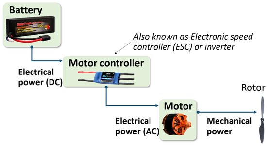
Figure 1.
An electric powertrain and its constituent components.
Practitioners will appreciate the validated powertrain models for SUAS powertrain analysis. The models rely on physics-based governing equations and physically meaningful parameters that a user can populate from an SUAS component datasheet. A user does not need to characterize any component empirically in order to model the component. This allows a user to quickly evaluate different commercial-off-the-shelf (COTS) motor, controller, and battery configurations under arbitrary loads without conducting time-consuming and costly experiments. Aerospace researchers will appreciate the novel propeller torque and rotational speed flight data. The data can validate other models for electric powertrains, rotor aerodynamics, and vehicle flight dynamics.
We contribute to the state of the art via novel analytical models, novel experimental methods, and novel experimental data. The rest of the paper further details each novel contribution.
Novel analytical models account for harmonic losses inside the motor and motor controller that similar studies have ignored [2]. Harmonic losses are induced when the motor-controller throttle setting is less than 100%. Small UASs tend to reach 100% throttle only during short maneuvring bursts, so harmonic losses are present during a majority of a vehicle’s flight and can significantly reduce powertrain efficiency [3] and thereby vehicle flight performance. Our harmonic-aware efficiency models enable practitioners to predict powertrain efficiency more accurately.
A novel wind-tunnel stand measured motor and controller efficiencies separately using a three-phase power analyzer. Other studies measured the combined motor–controller efficiency to reduce experimental complexity [4]. We present novel experimental measurements of the distinct motor and controller efficiencies for different motor–controller combinations under parametric loads. The separate efficiency data permit researchers to evaluate other powertrain models for the motor and/or controller.
A novel data acquisition system aboard a quadcopter directly measured the torque of one propeller during flight. Other studies estimated propeller torque using the controller’s DC current [5], but motor torque is proportional to motor current—not controller current. Therefore, we present novel experimental data of a quadcopter propeller’s torque collected during flight. Again, researchers can use the novel data to validate other electric powertrain or aerodynamic models.
Finally, we present a novel end-to-end validation of the models using the flight data. Given the upstream propeller torque and rotational speed, our integrated powertrain model predicts the battery’s voltage within 5% of measured values throughout a 5+ min mission. Other approaches rely on throttle and current lookup tables collected on the ground for specific propeller, motor, controller, and battery combinations. Our approach calculates the throttle and current on-demand from the upstream torque and rotational speed for an arbitrary motor, controller, and battery. The abstract torque and rotational speed can come from any type of propulsor, such as a propeller or a flapping wing, which can help researchers develop novel SUAS platforms, like robotic birds.
1.1. Motivation
An experimental optimization study demonstrated that current small UAS electric powertrains are sub-optimal [6]. Systematic testing of over 500 propeller, motor, and battery combinations yielded a 45-gram quadcopter with almost double the electrical power loading of a comparable commercial system. The optimized vehicle could hover for 31 min, which is an unprecedented flight time for a hover-capable aircraft at this scale.
Achieving such powertrain enhancements with analytical models rather than parametric experiments can help engineers at all stages of SUAS design. Rather than integrate components physically into an expensive test stand or flight vehicle, an engineer can simply plug its salient specifications from online datasheets into a virtual powertrain model and evaluate the component under expected loads or a simulated mission.
The models can help early-stage vehicle designers searching for the optimal powertrain configuration from a local library of parts. The designers can use the models to simulate each configuration’s entire mission performance and select the option that best achieves customer requirements. This step can be useful after the designer has identified a number of commercial parts that roughly meet size or mass constraints.
Alternatively, the models can also help late-stage systems engineers trying to improve an existing vehicle’s performance. For example, shrinking a quadcopter’s motors reduces overall vehicle weight and, thereby, the hover loads on the motor. However, smaller motors operate less efficiently and can draw more current from the battery [7]. Systems engineers can use the models to evaluate whether changing parts can improve flight performance.
1.2. Challenges
A user should be able to parameterize the models from hobbyist datasheets. Small UAS parts are often sourced from the hobbyist community, which provides minimal documentation for components. For example, documentation for a 5 kW SUAS motor only specifies the motor’s torque constant (), winding equivalent resistance (), and a static measure of no-load current () at an unspecified rotational speed [8]. On the other hand, documentation for a 50 kW motor suitable for manned aircraft specifies the aforementioned constants as well as the motor’s DQ-axes inductances (, ), rotational moment of inertia (J), and dynamic measure of no-load power across a range of rotational speeds () [9]. An SUAS motor model should expect that a user only knows a motor’s , , and .
Lackluster hobbyist documentation necessitates in-house experiments to validate models for different components. Some manufacturers tabulate data for thrust, rotational speed, and DC current for different propeller, motor, and controller combinations [8]. However, the manufacturers do not measure torque and efficiency, which are more salient to validating powertrain models. The manufacturers also do not list the specifications of the controller or power source used to conduct the tests.
Last but not least, the models should exclude the propulsor. That is, the most upstream input to the powertrain model should be mechanical torque and rotational speed—not the thrust of a traditional propuslor, like a propeller. Researchers are using battery electric powertrains to explore novel propulsion systems like cycloidal rotors [10]. Developing a propulsor-agnostic powertrain can also help those researchers. Traditional SUAS designers can integrate a propeller model from established aerospace literature, such as momentum theory or blade-element momentum theory [11].
1.3. Literature Review
Table 1 summarizes existing modeling solutions and highlights where our proposed models fit. The table is contextualized with respect to the motor since it is the most visibly active part of an electric powertrain.

Table 1.
A comparison of motor modeling and software tools.
On one extreme, there exist constant or ideal efficiency assumptions that are suitable only for the very initial sizing stages of aircraft design. Assuming some constant efficiency for the entire powertrain, such as , an aircraft designer can roughly estimate the battery energy required for a notional mission. The designer can then combine this assumption with first-order models like momentum theory to estimate the required battery mass for a notional mission. Powertrain sizing codes, like HYDRA, SUAVE, and NDARC, use this approach to populate the very first conceptual design [12,13,14]. This approach can only tell a designer that losses increase as demanded power increases.
On another extreme, there are detailed design tools like Motor-CAD or ANSYS Electronics suitable for the motor designers. These tools use detailed data to obtain rich information about motor losses at a single operating point. The inputs include the motor’s detailed geometry, such as lamination thickness, as well as constituent material properties and the fluid properties of the surrounding environment. These tools are useful to design novel high specific-torque motor topologies for electric aviation [15], but the tools are grossly inappropriate for aerospace users.
One tier below the motor design tools are software suites like Simulink, which are suitable for controls engineers developing a control system for a well-characterized motor. These dynamic modeling tools rely on a number of specifications—such as motor DQ axis inductances, moments of inertia, viscous damping, and a mapping of motor losses—to predict a motor’s transient dynamics [16]. At first glance, these tools may also seem appropriate for estimating powertrain losses; however, these tools provide too much detail at too high a cost. A vehicle designer or systems engineer is more interested in the steady-state or quasi-steady-state response of a motor. Moreover, SUAS motor manufacturers do not provide all the necessary data to parameterize these types of models. For example, viscous damping, inertia, and loss maps require careful testing on a dynamometer. Most hobbyists do not care for this info, so manufacturers do not test and publish these specifications. These tools are useful for modeling the coupled dynamics of a propeller and motor once the user has selected, acquired, and characterized a motor.
We propose an “in-between” approach that provides more nuance than constant efficiency assumptions without encumbering the user with the need to characterize the motor empirically vis-à-vis dynamic modeling tools. Our models use parameters readily published in SUAS specsheets—such as , , and for the motor—to predict steady-state losses. Our models capture how losses vary as torque, rotational speed, DC voltage, and the motor design vary. The lower-fidelity constant efficiency assumption simply assumes losses increase in proportion to output power. The open-source nature of our models also liberates users from having to use proprietary software like Simulink. Finally, our models’ most up-stream model inputs are torque and rotational speed, not propeller thrust, so a user can apply the model to a propeller or a flapping wing.
Other SUAS design tools in the literature require the user to pre-characterize each powertrain configuration. For example, a mission-based parts optimizer tool picks the best propeller, motor, and battery combination for a user-specified mission [4]. However, the user must provide test data for each propeller, motor, and battery in a local parts library. Users cannot evaluate a component’s efficiency using datasheet constants like the motor torque constant or battery capacity. Another mission-based optimizer tool numerically solves for a SUAS’ minimal-weight geometry. However, the tool assumes the user has already chosen the powertrain configuration and characterized the powertrain’s throttle-current response.
Powertrain-focused design tools still fall into the same pre-characterization trap. An engineer cannot parameterize models developed by Thurlbeck and Dehesa with only common motor specifications , , and . Thurlbeck had to measure the inductances required to populate their model [17], and Dehesa had to conduct parameter identification to populate the inductance and inertia terms in their model [18]. Effectively, the powertrain analysis models developed in these studies are closer to the dynamic models found in Simulink. As such, these models in the literature are impractical for vehicle designers and systems engineers who seek nuanced efficiency analysis without having to characterize each component.
Powertrain models developed by Gong almost achieve the desired fidelity and workload balance [2]. These models are parameterized from readily available datasheet specifications. However, the models are tuned and validated to a single motor and controller. Moreover, the models do not account for harmonic losses, which can drastically reduce the efficiency of the motor and controller. Additionally, the controller model is purely derived from empirical regression. This is understandable since SUAS motor controllers come with practically zero documentation. However, the authors did not attempt to derive a physics-based model that could be parameterized from a well-documented controller in the future.
Separately, the literature does not describe how to measure a small UAS’s powertrain dynamics in flight. Gong et al. described an in-flight thrust measurement system for a fixed-wing UAS, but they did not describe the electronics used to digitize and record this data [5]. Other researchers calibrated a vehicle’s thrust vs. motor throttle curve on the ground and estimated thrust from the applied throttle in flight ([19]). However, this approach only estimates dynamic flight loads from static ground tests, which is inaccurate. Larger vehicles measure the flight loads directly using strain-based sensors and digitize and record the data with onboard data acquisition systems [20]. Such data-acquisition equipment is too large and heavy for electric small UASs.
1.4. Outline
In the methodology section, we outline the hybrid modeling and experimental approach we undertook to develop and validate the proposed efficiency models. We also detail the novel experimental test setups we built to generate validation data for the models. In the subsequent Models and Results section, we discuss each component efficiency model in more detail and validate it against experimental data. We also integrate and validate the combined models against novel flight data. Next, we apply the models in case studies to solve common problems faced by vehicle designers and systems engineers. We conclude with a high-level discussion of our results, limitations, and suggestions for future work.
2. Methodology
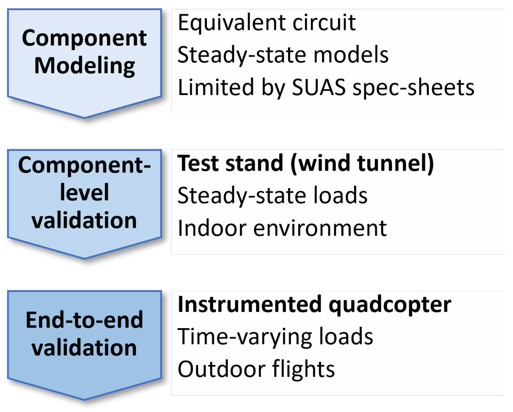
We approached the research problem in an increasingly broad manner, as abstracted in Figure 2.
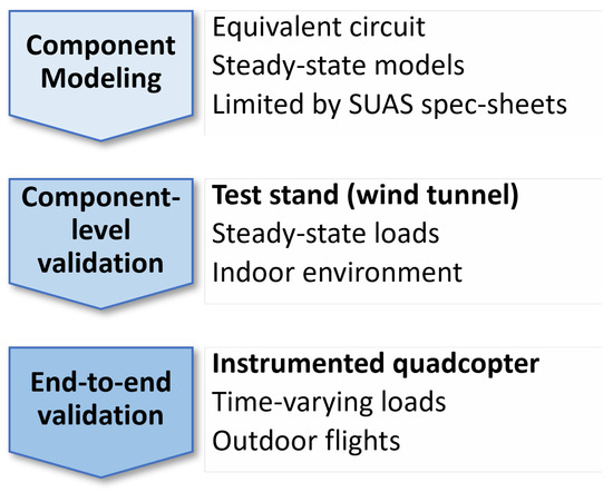
Figure 2.
The study methodology.
The novelty of our approach is in how we maximized our models’ predictive fidelity from the limited information provided by SUAS component datasheets. First, we explored fundamental electrical literature, such as textbooks, to understand the operating principles and losses of each powertrain component. The electrical literature uses equivalent circuits to derive efficiency models of various fidelity for each component. However, the challenge was to adapt the models such that a user could populate them using SUAS component datasheets while still capturing the nuances of each component’s efficiency. Section 3.1.2, Section 3.2.2 and Section 3.3.2 detail the tradeoffs we made for each component model to achieve the desired balance.
Next, we validated each component model against novel experimental data from a custom test stand. The stand, detailed shortly, was used to test each component under constant loads in a controlled environment. The novelty of the experimental test stand data stems from the separate measurements of motor efficiency and controller efficiency. Other studies measured the combined motor–controller efficiency [4] to save time and resources. This stand’s mechanical modularity allowed the testing of a variety of propeller, motor, and controller combinations. The modularity also enabled testing inside a wind tunnel, which allowed parametric load cases at different freestream velocities.
Finally, we validated the combined component models as an integrated powertrain model against novel experimental data from a specially instrumented quadcopter. The quadcopter, detailed later, was used to test the combined components under realy dynamic flight loads. The novelty of this approach is two-fold. First, the custom instrumentation and data itself are novel. The literature does not describe how to directly measure torque on a flying SUAS, and therefore, the literature does not contain flight data for SUAS torque. Second, the integrated model calculates instantaneous battery voltage from the time-varying propeller torque and rotational speed. Other approaches use pre-characterized look-up tables of throttle and current to estimate voltage [19].
2.1. Test Stand
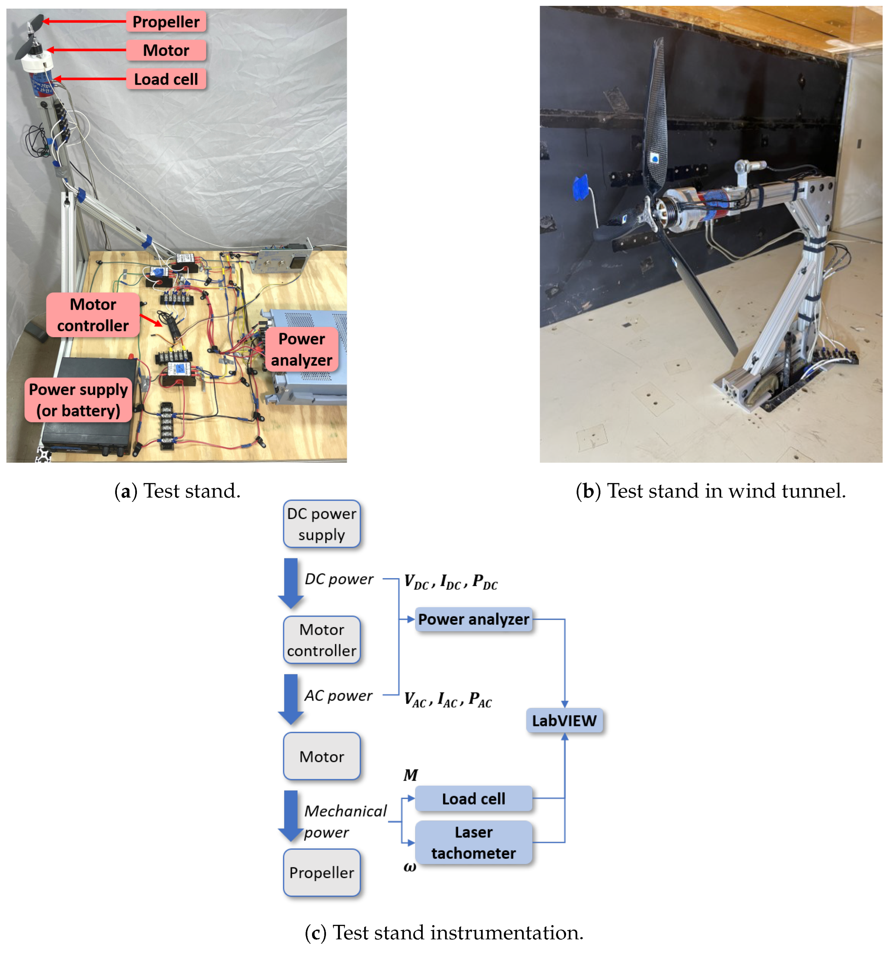
The test stand pictured in Figure 3 provided steady-state experimental efficiency data for each component. The stand accepted a variety of propeller, motor, motor controller, and battery combinations. The stand could be oriented vertically or horizontally, as seen in Figure 3a and Figure 3b, respectively. We conducted our tests in the horizontal orientation inside a wind tunnel, as shown in Figure 3b.

Figure 3.
Test stand setup.
The block diagram in Figure 3c shows the test stand’s complete instrumentation data flow. A torque sensor in line with the motor measured torque (M), and a laser tachometer measured rotational speed (). The product of these readings yielded the motor’s output power (, Equation (1)). An external pitot tube not visible in the images measured freestream velocity inside the wind tunnel.
The test stand instrumentation included a three-element power analyzer to measure electric power. Two elements measured electric power entering the motor (), and the third element measured electric power entering the controller (). Thus, the test stand instrumentation (Figure 3b) separately measured motor efficiency (, Equation (2)), and controller efficiency (, Equation (3)). Table A1 and Table A2 list the devices tested on the stand.
A three-element power analyzer (Yokogawa WT333E) was necessary because brushless DC motors macroscopically mimic multi-phase AC motors. At any instant in time, a single phase of current travels through a BLDC motor. However, the motor controller constantly re-routes this current along two of three wires (phases) of the motor. Thus, accurately measuring a BLDC motor’s input power requires at least a two-phase power analyzer (Blondel’s theorem [21]).
2.2. Instrumented Quadcopter
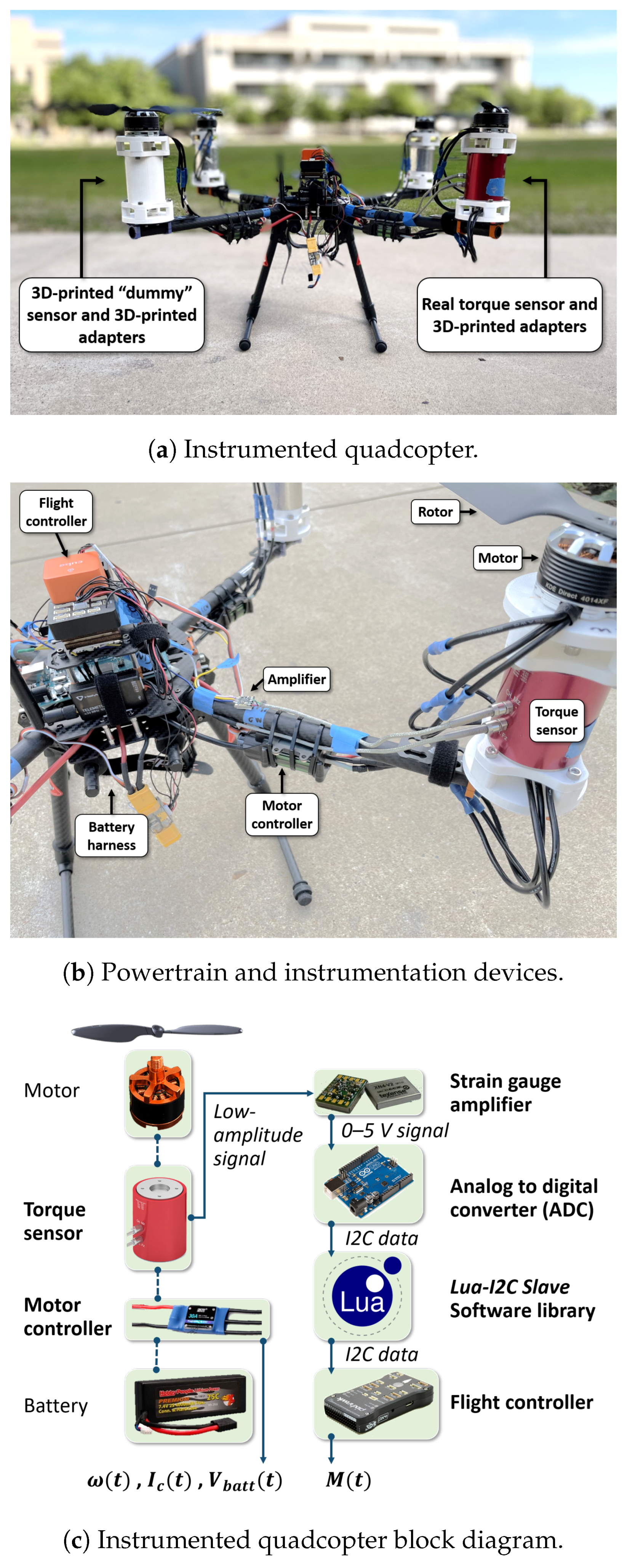
The specially instrumented quadcopter (Figure 4) provided flight-data to validate the powertrain model under dynamic loads. The onboard data acquisition system measured torque and rotational speed for the forward-left propeller-motor as well as the overall battery voltage. Reference [22] discusses the instrumented quadcopter in more detail.

Figure 4.
Instrumented quadcopter system.
The block diagram in Figure 4c shows the vehicle instrumentation’s data flow. The data flow consisted of two data streams: a data-logging system built into the motor controller and the novel external torque measurement system. The built-in system used the data-logging feature of the motor controller to record rotational speed and battery voltage directly onto the motor controller’s memory.
The novel torque measurement data stream used commercial hardware and open-source software to measure and record torque onto the flight controller’s memory card. The software can accommodate additional sensors, such as thrust and torque cells for multiple propeller arms. The data flow consisted of the following:
- Torque sensor (Futek MBA500), which measures torque up to 5.6 N·m (50 lb·in).
- Strain-gauge amplifier (Texense XN4-v2), which excites the torque sensor and amplifies and offsets the resulting output voltage into a 0–5 V analog signal.
- Analog-to-digital converter (ADC) (Arduino Mega), which digitizes the torque signal. Commercial flight controllers, like the Cube Orange, do not have 0–5 V analog inputs.
- Software bridge (I2C Slave library), which transfers the digitized torque voltage from the Arduino to the flight controller via an I2C bus.
- Flight controller (CubePilot Cube Orange), which stores the torque voltage datastream onto a memory card.
The vehicle itself was a 3.7 kg (8.2 lb) quadcopter with an estimated thrust-to-weight ratio of 3.2 at full throttle. The footprint was 65.0 cm (25.6 in). The rotors were two-bladed propellers with a diameter of 38.1 cm (15 in) and a pitch of 5.5 degrees. A KDE Direct 4014XF-380 motor powered each propeller, and a Castle Phoenix Edge 60 electronic speed controller (ESC) controlled each motor. A single 6 A·h, 6S (25.2 V peak) battery supplied power to all four motor systems. The vehicle had a number of custom 3D-printed dummy sensors and mechanical adapters. Each dummy sensor had the same volume and nearly the same mass as the real sensor to balance the vehicle inertia.
3. Models and Results
We present each component efficiency model and validate its predictions against experimental measurements from the test stand. Each model has two sets of inputs: (1) external settings, like the applied torque, and (2) datasheet specifications, like winding resistance.
Next, we combine the component models into an integrated powertrain model and validate its predictions against experimental flight data from the instrumented quadcopter. The inputs are (1) the externally applied propeller torque and rotational speed time histories and (2) the datasheet specifications of the constituent components.
All the models are size-agnostic because the physics-based internal specifications inherently scale with size.
3.1. Motor Model
A motor has three sources of inefficiency: resistive losses, which grow with torque; iron losses, which grow with rotational speed; and harmonic losses, which stem from voltage modulation [7]. Motor resistive losses are analogous to an aircraft’s induced drag. Resistive losses are a by-product of generating torque just as induced drag is a by-product of generating lift. Conversely, iron losses—also known as no-load losses—are analogous to an aircraft’s parasitic drag. Iron losses increase with rotational speed just as parasitic drag increases with forward velocity. Harmonic losses occur when waveform harmonics at partial throttle (throttle < 100%) generate heat without contributing to useful work in the motor or the motor controller.
Equation (4) is the salient equation of the motor efficiency model, which captures the three main losses. The user must supply the following:
- Three external parameters—applied torque (M), rotational speed (), and DC voltage (). A user populates these from the expected load and the system bus voltage.
- Three internal parameters—torque constant (), equivalent winding resistance (), and no-load current (). All these parameters are published in SUAS motor datasheets.
The output power term () is a product of the applied torque and rotational speed. The resistive losses () are the product of the ideal current draw () and the equivalent resistance of the motor’s winding. The iron losses () are the product of the torque constant, rotational speed, and no-load current. The duty ratio () amplifies resistive and iron losses when to model harmonic distortion from modulating voltage () at partial throttle settings. A 10% penalty to the denominator’s output power term captures high-order iron losses, which we detail in the discussion. The motor’s true current draw () is a function of the motor’s input power, DC voltage, and duty ratio ().
3.1.1. Validation
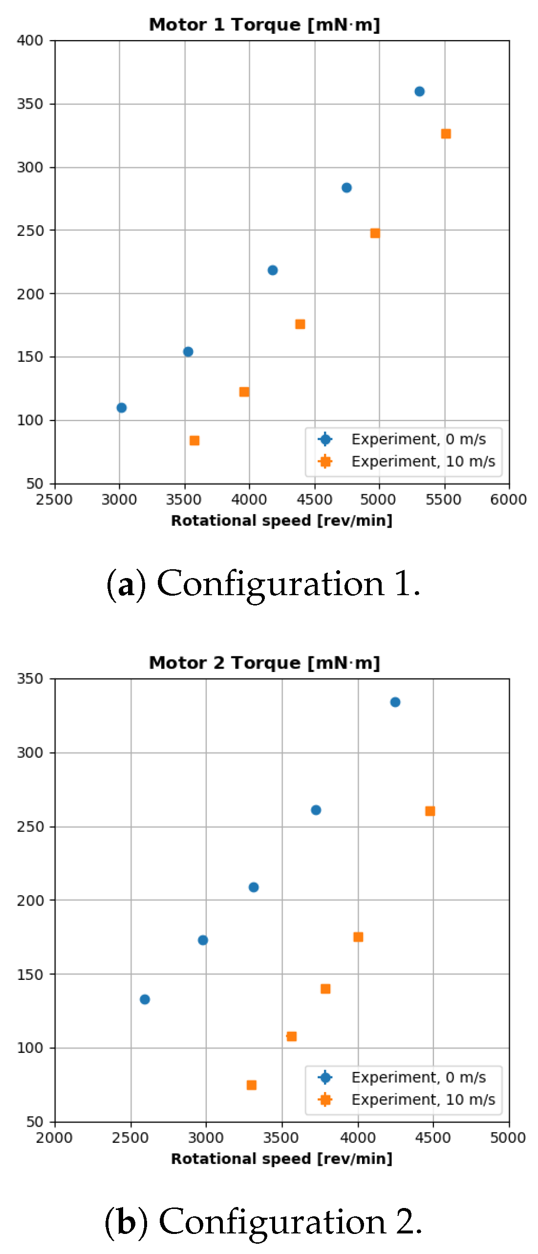
Figure 5 plots the mechanical load profile of four different brushless DC motors and motor controllers on the test stand. A fixed-pitch propeller of varying diameter provided the mechanical load at freestream velocities of 0 m/s and 10 m/s. For a constant rotational speed, the motor torque decreased when freestream airflow was present because the axial flow would reduce the propeller blades’ angle of attack and, thereby, reduce the torque load on the motor. This experimental torque and rotational speed data were fed into the motor efficiency model (Equation (4)). Table A1 in Appendix A contains the specifications of the tested components.
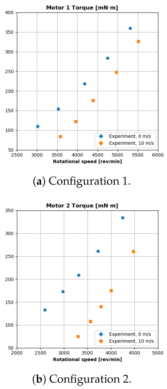
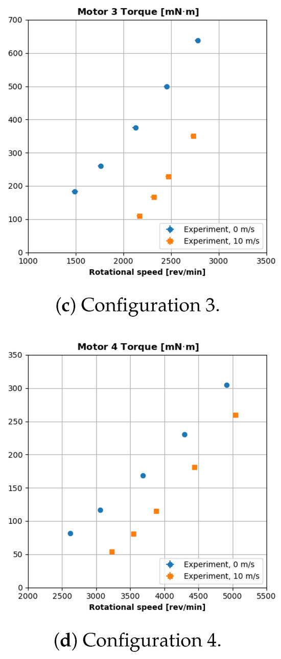
Figure 5.
Mechanical load profiles for different motor–controller configurations.
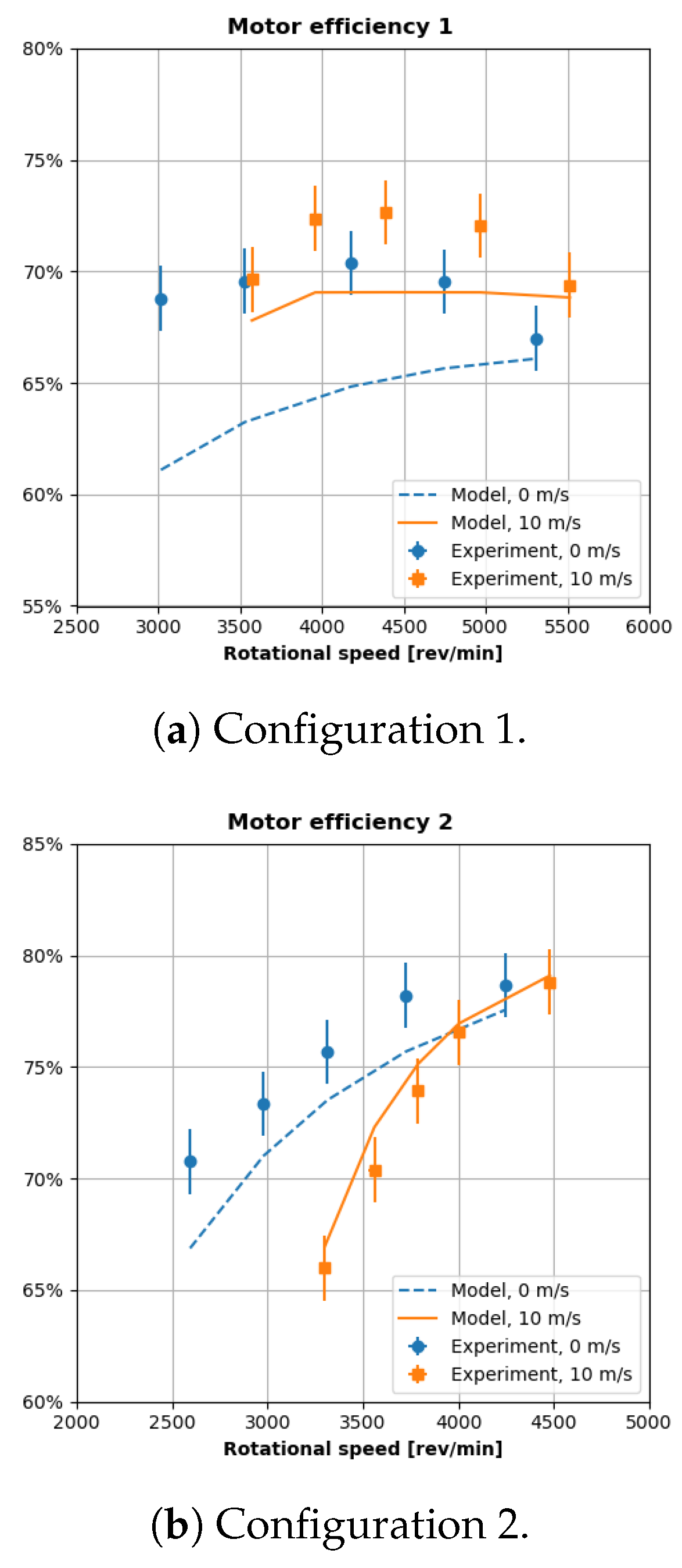
Figure 6 plots the corresponding motor efficiency profiles for the tests in Figure 5. Each sub-figure in Figure 6 plots the experimental measurements and our motor model predictions for each load profile (0 and 10 m/s).
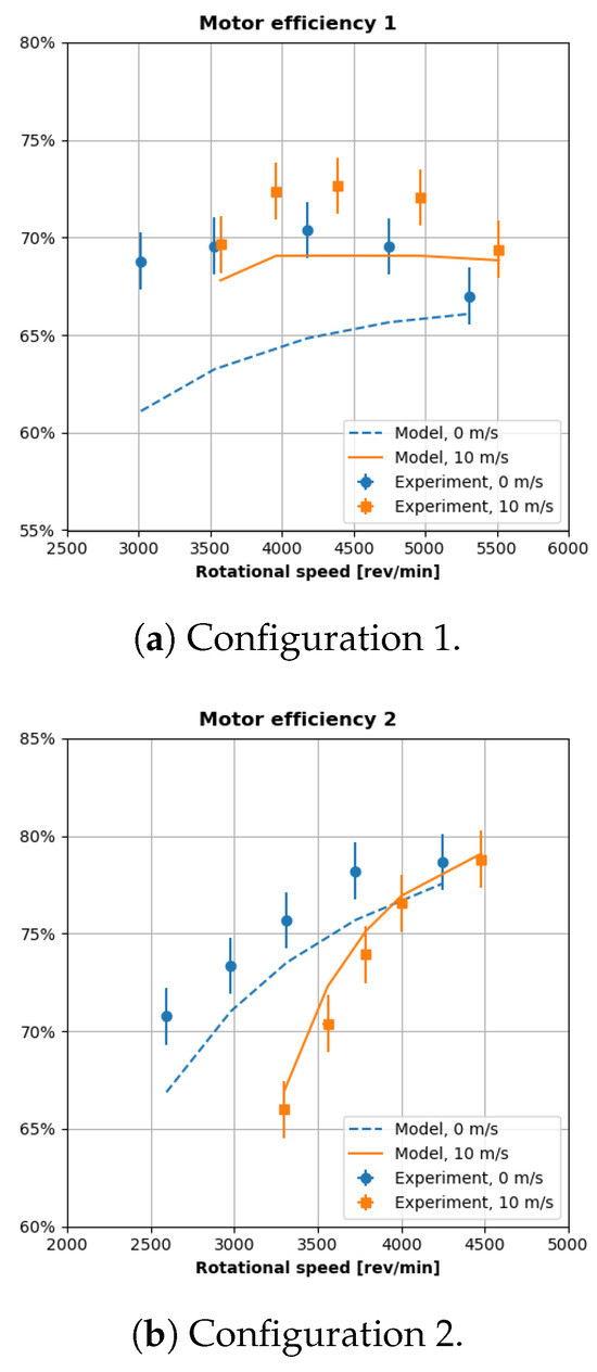
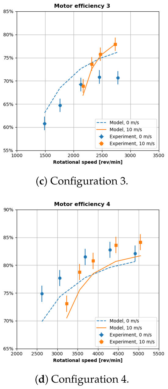
Figure 6.
Motor efficiency profiles for different motor–controller configurations.
The experimental measurements exhibit similar trends to data collected by Gong [2]. The motor efficiency is markedly less than the popular assumption of 90%, and the efficiency tends to increase as rotational speed decreases. Some of our experimental measurements captured peaks and subsequent drop-offs in motor efficiency, such as the peak that occurs for the 10 m/s case in Figure 6a. However, Gong’s experimental results did not capture any peaks in efficiency. The presence or lack of a peak efficiency value is merely a coincidence in the different load profiles used to test the motors and does not reflect a deficiency in either study.
Our model precisely captures changes in the motor’s efficiency profile. For example, the minimum measured efficiency in Figure 6b decreases from 70% to 65% as the wind tunnel flow increases from 0 to 10 m/s. The maximum measured efficiency does not change between the two cases. The predicted efficiency curves roughly match these changes. The minimum predicted efficiency decreases from 68% to 65% as the wind tunnel velocity increases from 0 to 10 m/s, and the predicted maximum efficiency does not change.
The motor model predicts efficiency accurately within 10% of measured values. The worst-case predictions are in Figure 6a. The model under-predicts motor efficiency by about seven percentage points at 3000 rev/min, 0 m/s. This absolute difference corresponds to a relative difference of about 10% with respect to the measured motor efficiency (70%).
3.1.2. Discussion
Our approach sacrifices some fidelity to ensure engineers can use the model without experimental pre-characterization. In Figure 6a, the 0 and 10 m/s experimental efficiency curves peak around 4200 and 4400 rev/min, respectively, before gradually decreasing. However, our model predictions merely plateau and do not decrease like the experimental profiles. This is a limitation of relying on the constant to model no-load losses. Hobby manufacturers provide as a static snapshot of no-load losses at an unspecified rotational speed. However, the electrical literature shows that no-load losses vary with and [23]. Gong measured the change in as a function of for their test motor and incorporated this information into their no-load loss term [2]. However, this approach requires a user to experimentally characterize each motor they wish to model. We pursued a less accurate but more general solution by applying a 10% penalty to the denominator’s output power term to reclaim some of the higher-order iron losses, as recommended in [24]. Similarly, the electrical literature uses more complex Fourier methods to calculate non-linear harmonic losses [25]. We approximate harmonic losses with the duty-ratio amplification factor since modulating voltage is a strong function of duty ratio (throttle).
Nevertheless, our motor model improves on the existing literature. The aerospace literature often assumes a constant and ideal 90% efficiency for the combined motor and controller [12] or requires that a user provide the efficiency data for a particular powertrain. Our model can predict a motor’s changing efficiency within 10% of measured values using high-level motor specifications. Even in the worst case, Figure 6a, our model only under-predicts efficiency by seven percentage points (63% vs. 70% at 0 m/s) or about 10% of the actual efficiency (70%). In contrast, the error in the popular 90% efficiency assumption (20 percentage points) is almost 30% of the experimental efficiency!
The improvements in efficiency prediction have significant implications at the vehicle level. Using the previous set of numbers, a vehicle designed with our code would carry a 10% oversized battery and still likely achieve its desired mission. However, a vehicle designed with the constant efficiency assumption would carry a 30% undersized battery and more likely would not achieve its mission.
An SUAS conceptual designer can use our motor model as a sanity check within the first few design steps. First, a designer can size a hypothetical motor using sizing codes like SUAVE [13] or NDARC [26]. Next, the designer can find commercial motors that best match the ideal size requirements. At this point, the designer can populate our model with the salient datasheet specs and evaluate the candidate motors under expected loads without running any characterization experiments. The user can then select the most efficient motor and size the battery to a more realistic powertrain efficiency figure.
Our motor model is also applicable to newer, high-specific torque motors, like axial-flux motors. Brushed DC motors, brushless DC motors, and permanent magnet synchronous machines (PMSMs) are fundamentally the same type of motor, so the model can predict efficiency for all three aforementioned motor designs. Manufacturers can build these three motors in axial- or radial-flux topologies, yet this difference only affects the strength of the magnetic interactions inside the motor (the value of )—not the operating principles of the motor. Therefore, the motor model is also flux-agnostic. The motor model does not work for induction or reluctance motors, which operate on different principles.
3.2. Controller Model
A controller has four sources of inefficiency: resistive losses associated with current, switching losses associated with multiple parameters, harmonic losses, and standby power losses [25]. The controller’s resistive losses are most closely related to the mechanical load: higher torque generally increases controller resistive losses. The controller’s switching losses are more related to system settings, such as the selected DC bus voltage [27]. Just like in the motor, harmonic losses also bleed in from modulating powertrain throttle. The standby losses stem from powering the controller’s various internal circuits.
Equation (5) is the salient equation of the controller efficiency model. The user must supply the following:
- Three external parameters—motor power draw (), motor current draw (), and available voltage (). A user can populate these parameters using the predictions of the motor model.
- Four internal parameters—switch resistance (), pulse-width modulation frequency (), switching delay (), and standby power ().
We recommend = 1 m, = 200 ns, = 12 kHz, and = 0.5 W. Manufacturers do not produce SUAS controllers in as many varieties as motors, and the controllers rarely come with any documentation. One controller manufacturer, Jeti, publishes 1 m for some of its controllers [28]. A datasheet for an electrical switch similar to those found in SUAS motor controllers suggests 200 ns [29]. The default value for most controllers’ 12 kHz [28]; however, users can sometimes adjust this value by re-programming the controller’s firmware. Our tests indicated 0.5 W.
Users can supply our models with more accurate parameter values in the future. SUAS parts manufacturers should provide more rigorous documentation to meet certification demands for electric aviation.
The controller’s resistive losses () are the product of the motor’s input current and the controller’s switch resistance. The controller’s switching losses () are the product of the controller’s pulse-width modulation frequency, the switching delay, the motor’s input current, and the DC voltage. The duty ratio again amplifies resistive and switching losses to model harmonic losses. The controller’s standby power models the power drain by the controller’s secondary circuits. The controller’s input current () is a function of the controller’s input power and the DC voltage ().
3.2.1. Validation
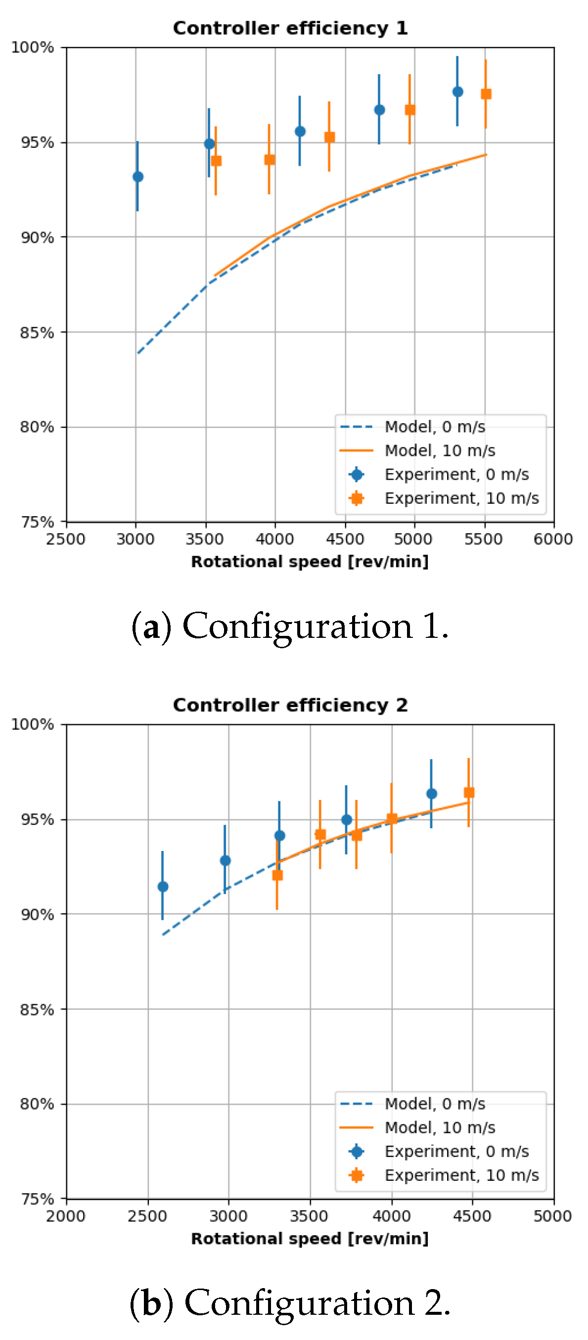
Figure 7 plots the corresponding controller efficiency profiles for the experiments conducted in Figure 5 and Figure 6. Each sub-figure in Figure 7 plots the experimental measurements and our controller model predictions for the different load profiles (0 and 10 m/s).
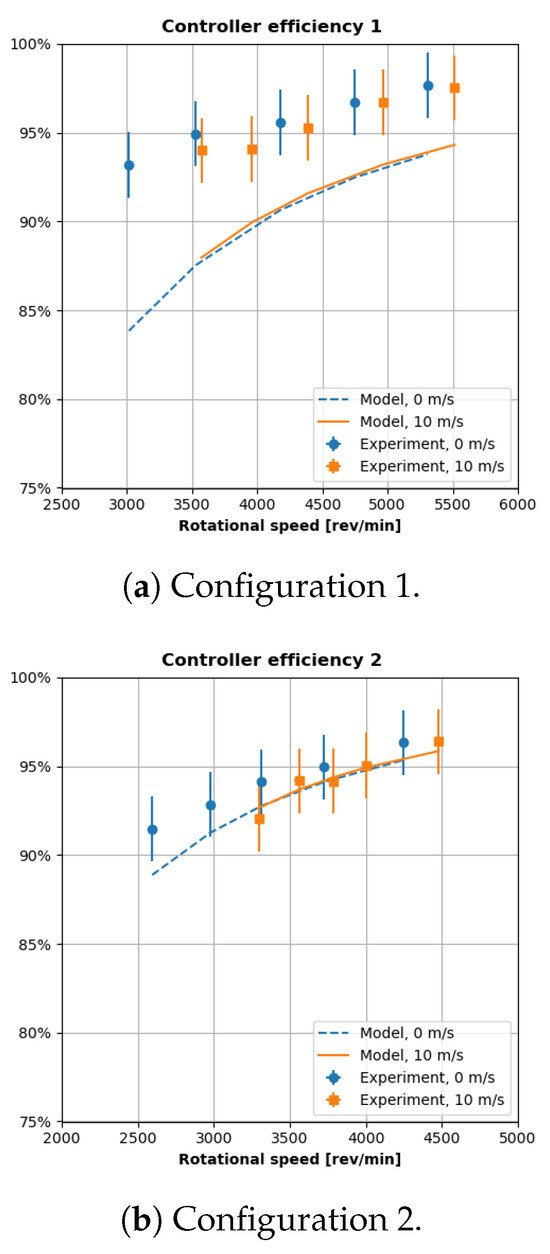

Figure 7.
Controller efficiency profiles for different motor–controller configurations.
Like motor efficiency, our controller efficiency measurements are similar to measurements by Gong. Moreover, the popular assumption of 90% efficiency is valid for the controller because the measured efficiency exceeds 90% in almost every case. Moreover, the measured controller efficiency does not experience a peak plus roll-off in any case. The controller efficiency increases with rotational speed in all cases.
In terms of accuracy, our controller model generally over-predicts losses and under-predicts efficiency for the 0 m/s profiles. In the worst case (Figure 7a), our model under-predicts controller efficiency by 10 percentage points (85% vs. 95% efficiency at 1500 rev/min). This absolute difference corresponds to a relative difference of 10%. Our model is generally more accurate for the 10 m/s profiles.
In terms of precision, our controller model matches the experimental trends in all cases despite the fact that we parameterized the model with values from similar devices—not the unpublished specifications of the device under test.
3.2.2. Discussion
Our controller model sacrifices some accuracy for robustness. Thurlbeck developed a high-fidelity physics-based controller model. The model can work for any controller, but it requires detailed information about the controller’s switches, such as gate driver voltage [17]. Unfortunately, almost all SUAS motor controllers come without any datasheets. Gong, on the other hand, developed a purely empirical regression model tuned for a specific controller [2]. We pursued a middle ground. We developed a physics-based model with fewer inputs, and we recommend reasonable values for these inputs based on what limited data are available for controllers and their switches. Unlike Gong’s model, our approach is immediately usable for any controller—not just the controller in their study. Moreover, our model, like Thurlbeck’s model, can be easily parameterized with more accurate specifications once rigorous controller datasheets are published.
Again, our model improves on the existing literature. The aerospace literature assumes a constant efficiency for the combined motor and controller [12], or some literature requires that a user provide the efficiency data for a particular powertrain. For the first time, the motor controller model can predict the changing efficiency of a controller using a few high-level specifications. The user does not have to experimentally develop an empirical regression for each controller like in the research by Gong [2].
At the vehicle design level, our model’s precision can improve how concept designers conduct tradeoff analysis for different operating conditions. The experimental results show that a controller’s efficiency is usually greater than or equal to 90%, so users can assume an ideal and constant 90% controller efficiency. However, our model can provide further insight into how that efficiency may change for different operating conditions. For example, assuming a controller efficiency of 90% may suffice to analyze the powertrain of a large and lumbering cargo SUAS with fairly constant cruise conditions. However, our model is more appropriate for analyzing the powertrain of a small and nimble surveillance SUAS, which experiences large swings in propeller torque and speed.
The controller model works best for brushless DC motor controllers, which use square-wave commutation. Users can apply the trends to permanent-magnet synchronous motor controllers, which use sinusoidal commutation (field-oriented control). Both types of controllers employ the same hardware to control nearly identical motors.
3.3. Battery Model
Batteries have multiple losses, but most of these losses occur at timescales far slower or faster than the mechanical timescale of an SUAS mission. For example, select transient losses occur in microseconds, while self-discharge losses occur over the course of months [30].
Equation (6) only captures the series resistance loss that occurs at the mechanical timescale of a flying vehicle. The user only needs to provide the external current draw (), the rated internal capacity (), the number of cells in series (), and the internal cell resistance (). All of these parameters are available in SUAS battery datasheets.
The first term represents the ideal voltage that cells inside the battery generate at a particular state of charge (). The second term represents the internal losses of the battery as the product of the total current and the battery’s internal resistance. Reference [31] defines as a non-linear function of and for lithium-based chemistries. The total number of cells in series inside the battery () scales both terms.
3.3.1. Validation
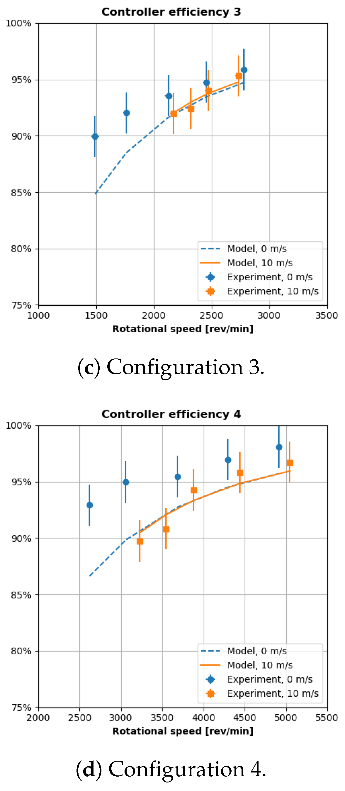
Figure 8 plots the measured and predicted battery voltages for three batteries. In each sub-figure, the x-axis is the relative discharged capacity (depth of discharge or DOD), and the y-axis is the per-cell voltage (total battery voltage per number of cells in series).
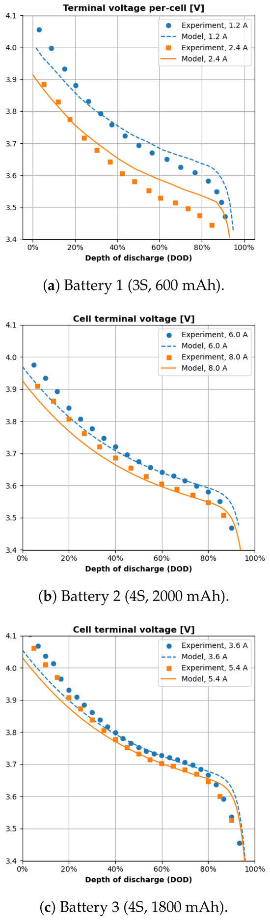
Figure 8.
Battery model validation for different batteries.
Each battery was discharged at two different discharge rates. Battery 1, a 0.6 A·h unit, was discharged at 1.2 A and 2.4 A, which correspond to double (1.2/0.6) and quadruple (2.4/0.6) its rated output current. Battery 2, a 2 A·h unit, was discharged at 6 A and 8 A, which correspond to triple and quadruple its rated current. Battery 3, a 1.8 A·h unit, was discharged at double and triple its rated current. Table A2 in Appendix A contains the specifications of the tested batteries.
The experimental measurements reflect the trends in the literature. As the discharge rate increases, more battery energy is wasted across its series internal resistance, which reduces the voltage available to the load.
The battery model predicts voltage within 5% of experimental values throughout the test domain for all batteries and all test cases.
3.3.2. Discussion
Compared to the electrical literature, our battery model is easier to populate. Our model requires two battery specifications—battery capacity () and internal resistance ()—both of which a user can obtain from reputable battery datasheets. The popular shepherd model requires three more constants that not all datasheets provide [32]. A user can directly provide the current time history () or estimate this input using our proposed motor and controller models. A user can even model other battery chemistries if they populate the appropriate function for the desired chemistries.
Moreover, our battery model only simulates losses that are relevant to aircraft design timescales. The electrical literature describes methods that characterize battery discharge in higher fidelity [30], but these discharge modes occur at timescales that are much shorter or much longer than an aircraft mission. As such, our model does not waste time and resources to simulate irrelevant losses.
At the vehicle design level, our battery model enables a user to evaluate a battery’s effective energy density for each mission. Initially, an engineer may size a concept vehicle’s battery, assuming constant energy density. Then, the engineer may identify candidate commercial batteries that roughly satisfy the desired size and mass constraints. Next, the engineer can evaluate how each battery performs under the expected mission loads using our model and the candidate batteries’ specifications. If a candidate battery depletes before the end of the mission, then that battery is undersized. If a candidate battery has excess voltage at the end of the mission, then that battery may be too large. Unlike the constant-energy density assumption, our approach captures how a battery wastes load-dependent portions of its own energy across its internal series resistance.
3.4. Integrated Powertrain Model
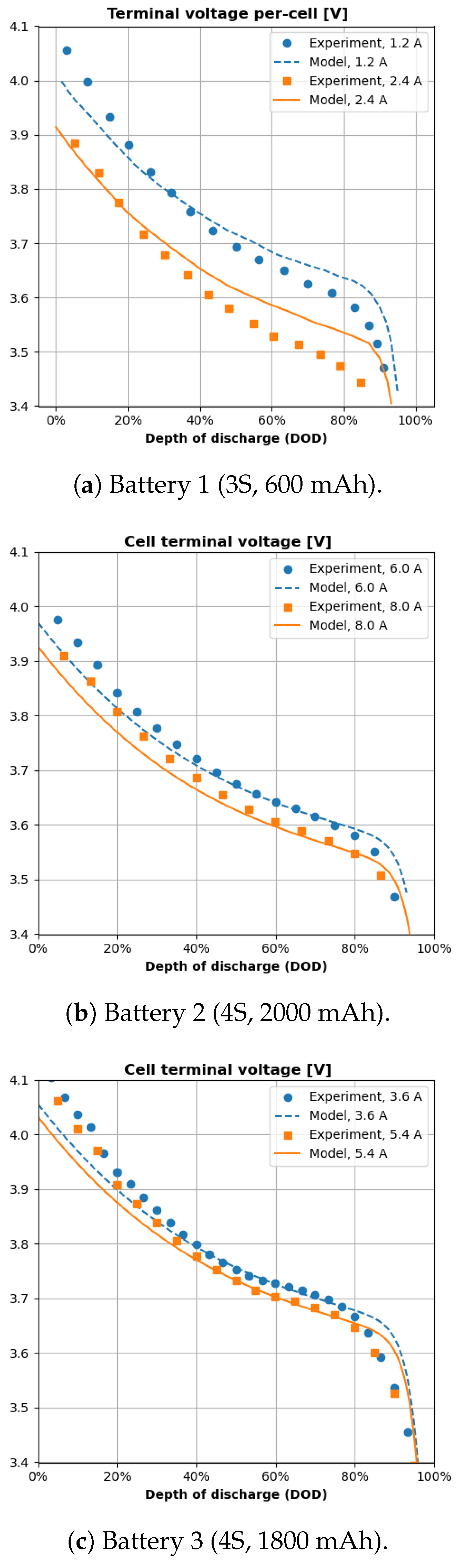
Figure 9 details how the component efficiency models are integrated into a quadcopter powertrain model. The most upstream model inputs are the vehicle’s propeller torque and rotational speed time histories. Each component model is parameterized with salient datasheet specifications, like torque constant, switching frequency, and the rated battery capacity.
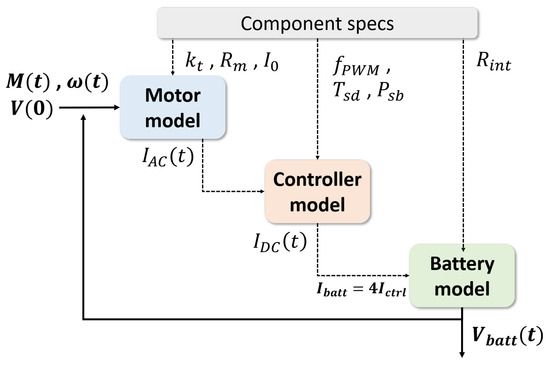
Figure 9.
Implementation of the powertrain models.
First, our model reads the initial battery voltage (), torque (), and rotational speed () data points. The motor model predicts the motor’s losses and the motor’s total power draw. Next, the controller model predicts the downstream controller losses and the controller’s total current draw. The integrated model assumes that all four controllers (propellers) draw the same amount of power from the battery. Then, the battery model applies the combined load from all controllers to the battery and predicts the new battery voltage, which starts the next iteration. The simulation steps forward in time until the battery reaches a 20% state of charge or a cutoff voltage of 3.3 V per cell.
3.4.1. Validation
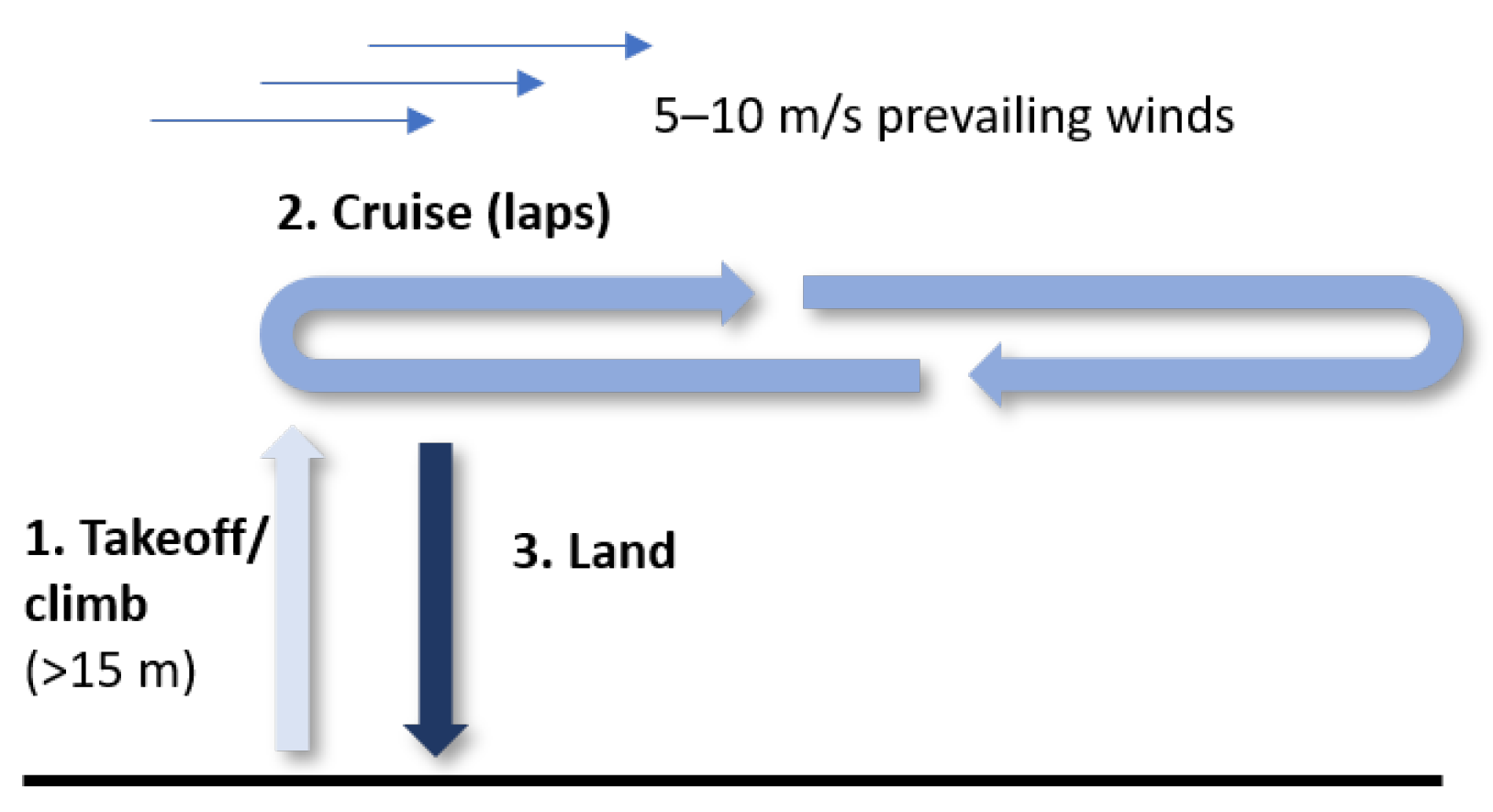
Figure 10 shows the flight plan for the instrumented quadcopter’s outdoor flight. The vehicle took off, climbed to roughly 15 m (50 ft.), and began flying 100 m (328 ft.) laps. The prevailing winds exceeded 5 m/s (10 kts), and the vehicle flew with the wind for half the lap and against the wind for the other lap half. The vehicle flew for almost 6 min before the pilot noticed sluggish performance that indicated a near-depleted battery.

Figure 10.
Flight plan of the instrumented quadcopter.
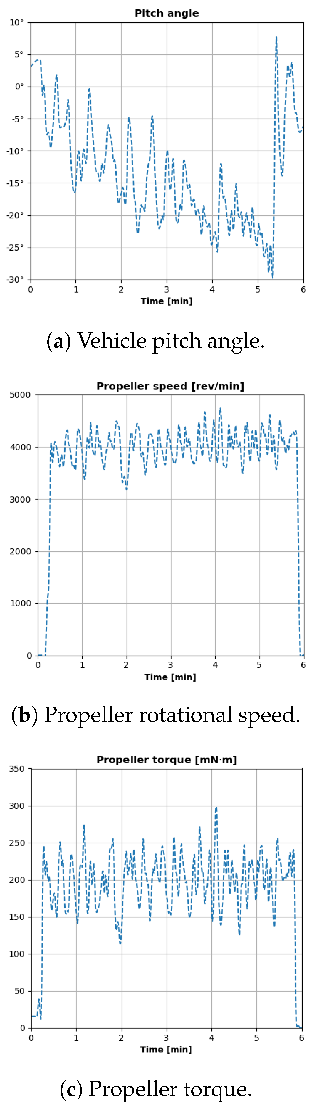
Figure 11 plots select flight data collected by the instrumented quadcopter. Figure 11a plots the vehicle’s pitch angle. The pitch angle is almost always negative because the quadcopter was flying forward with its nose pitched down. Figure 11b,c plot the rotational speed and torque, respectively, of the quadcopter’s forward-left propeller. All of these parameters oscillated as the vehicle flew against and with the wind. The torque data exhibit similar trends as the speed data since torque is proportional to rotational speed.
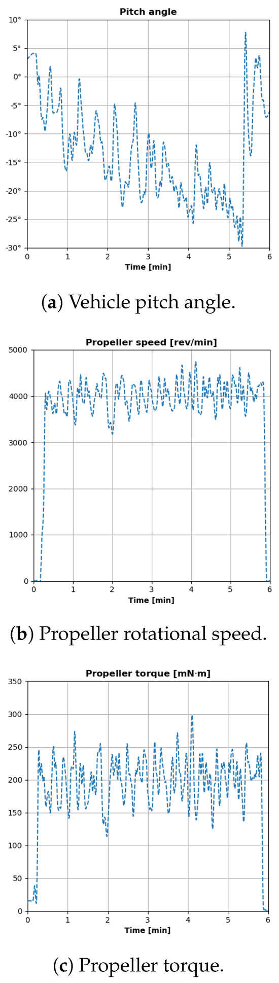
Figure 11.
In-flight quadcopter data.
Figure 12 plots the battery voltage measurements from the flight. The battery voltage experienced a stepped decrease in the beginning as the vehicle took off and climbed. This sharp drop stemmed from the four quadcopter arms simultaneously pulling a large amount of current across the battery. The voltage then decreased more slowly as the vehicle entered cruise. The voltage experienced periodic oscillations like the other flight measurements in Figure 11 as the vehicle flew windward (against the wind) and leeward (with the wind).
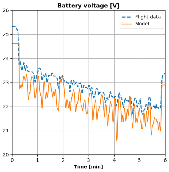
Figure 12.
Battery flight data vs. model predictions.
Figure 12 also plots the integrated powertrain model’s voltage prediction. The combined motor, controller, and battery models predict the vehicle’s voltage time history within 5% of in-flight measurements throughout the entire mission. We hypothesize the predicted voltage oscillated more dramatically than the measured voltage because of instrumentation limitations. The model only has mechanical data for a single propeller, so it assumes all four propellers experience uniform loading. In reality, each propeller experienced slightly different loads, and the loading variations across all propellers probably dampened some of the total current demand on the battery.
3.4.2. Discussion
Our component models’ fidelity is sufficient for power and efficiency analysis by vehicle designers and test engineers. Our combined models predicted battery voltage accurately in a dynamic outdoor flight despite the limited input parameters. The accuracy is even more remarkable since the integrated model must contend with two types of error propagation: propagation “down” the powertrain from the motor to the battery and cumulative propagation “through” the simulation time history.
At the aircraft design level, our models enable engineers to virtually optimize the entire powertrain for a given mission. Now, a user can analyze different powertrain configurations from end to end (propulsor torque to battery voltage) using commonly published component specifications rather than using experimental data like other literature studies [6]. This is extremely valuable once a user has identified a number of candidate parts that meet initial sizing requirements. The user can also conduct trade studies for different voltage settings or vehicle configurations (e.g., quad- vs. hexa-copter) and examine the impact on every mission phase. Our models offer more nuance than constant efficiency assumptions without encumbering the user with as many input requirements as proprietary Simulink or AMESim models.
4. Case Studies
We showcase how our validated efficiency models can deliver unique insights at the vehicle design level. Three independent and hypothetical cases are inspired by real scenarios. The first case shows how the models can inform decisions for an existing vehicle, not just a paper concept. In the second case, the models reveal nuances about voltage and efficiency that conventional wisdom does not capture. The third case shows how the powertrain models can even inform decisions about other vehicle aspects, like aural signature.
4.1. Case 1: Reducing Vehicle Weight
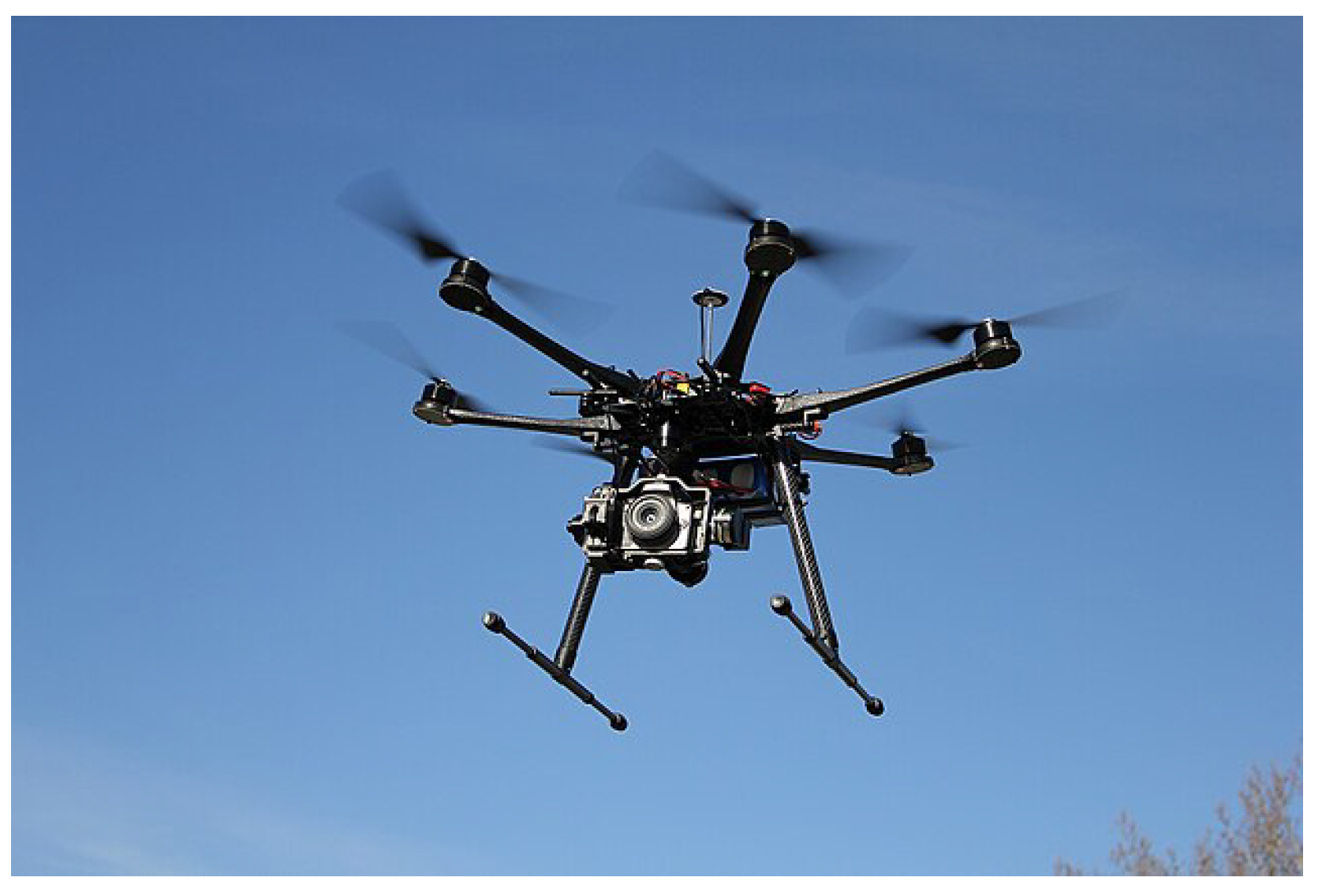
A systems engineer has been tasked with reducing the gross weight of an existing heavy-lift hexacopter (example in Figure 13) to increase its endurance. The engineer suspects that the original motors were oversized, so installing smaller motors can reduce the gross weight. However, the engineer is concerned the smaller motors may instead draw more current from the battery since efficiency decreases with size [7]. The engineer wants to evaluate the new motors without having to buy and test them.
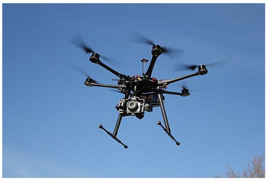
Figure 13.
Notional hexacopter for Case 1 (photo by A. Glinz, Wikimedia).
Table 2 lists the salient information known by the engineer for the oversized motors configuration (Configuration 1) and the proposed lighter motor configuration (Configuration 2). Except for the motors, everything in the two configurations is the same, including the propellers, motor controllers, and the main battery. The engineer calculates the new hover torque and rotational speed from in-house propeller data. The only unknown is the DC current for the new configuration.
Table 2.
Salient hexacopter information.
We can quickly solve this problem using our validated models. First, we solve for the motor’s efficiency using Equation (4). We populate the expression using the expected loads and motor specifications listed in Table 2. We then propagate the predicted motor values into our controller model and calculate the controller’s DC current draw. We parameterize the controller using the values recommended in Section 3.2. We ultimately obtain a DC current of 5.6 A for the second, lighter configuration.
The smaller DC current for the second configuration confirms that installing smaller motors will, in fact, increase vehicle endurance. The smaller current will not only draw less power from the battery but will also generate fewer losses across the battery’s internal series resistance and, thereby, increase the battery’s effective energy density. Now, the systems engineer can confidently swap motors.
A user cannot attain such insights using other approaches in the literature. The constant efficiency assumption does not distinguish between different motors. Powertrain models developed by Gong [2] and Thurlbeck [17], as well as high-fidelity modules in Simulink, require experimental tuning of the new motor, which defeats the purpose of using a model to predict performance in lieu of experimental testing.
4.2. Case 2: Increasing Overall Efficiency
For basic circuit elements, like a resistor, increasing the applied voltage reduces resistive losses ( or ). However, the same principle does not always apply to a more advanced circuit, like an electric powertrain. Sometimes, increasing the applied voltage can actually increase losses and reduce overall efficiency.
Figure 14 shows two efficiency contours of a brushless DC motor with = 29 mN·m/A, = 44 m, and = 0.7 A. Equation (4) is used to calculate the motor’s efficiency for each torque–speed point in each plot window.
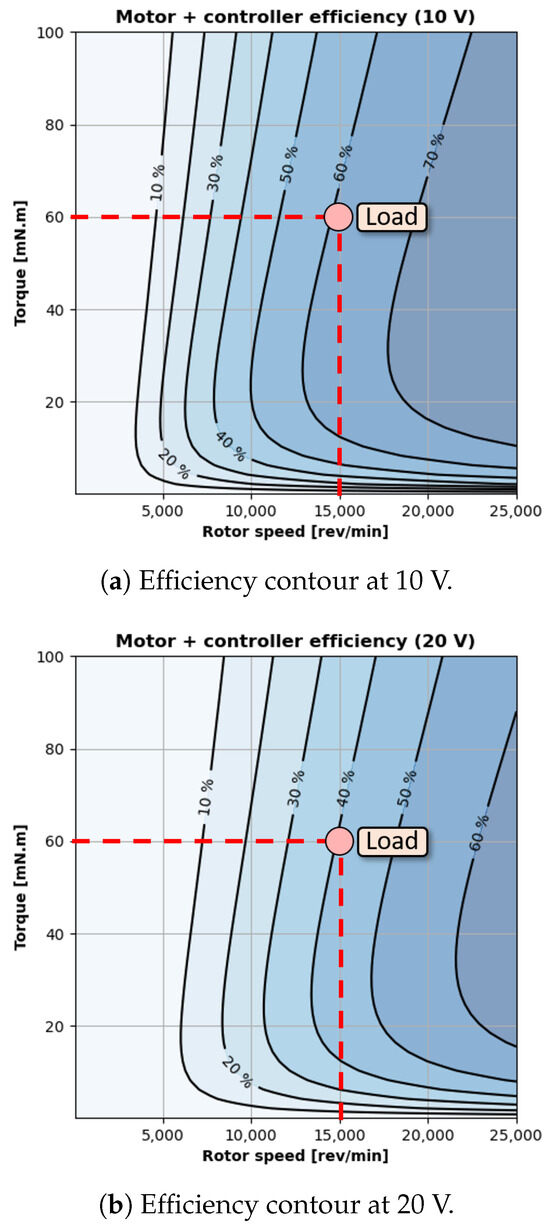
Figure 14.
Increasing voltage can decrease efficiency.
Figure 14a predicts the efficiency contour with a supply voltage of 10 V. The efficiency generally increases with torque and rotational speed, and the efficiency exceeds 70% within the plot window. The plot also overlays a hypothetical load point at 15,000 rev/min and 60 mN·m. This hypothetical load can be a quadcopter’s rotor in hover or a fixed-wing drone’s propeller in cruise. The motor drive system operates at approximately 60% efficiency at this point.
Figure 14b predicts the efficiency contour of the same motor with double the supply voltage (20 V). Again, the efficiency generally increases with torque and rotational speed. However, the peak efficiency is now less than 70%. Increasing the supply voltage has decreased the overall efficiency because the upstream controller must modulate the voltage and current waveforms to achieve the same torque and rotational speed given a higher supply voltage. Consequently, the motor experiences higher harmonic losses and a reduction in efficiency. The motor’s efficiency has decreased to 40% at the hypothetical load point.
These results are insightful in the initial design stages when an aircraft designer is conducting trade sweeps for system parameters like bus voltage. Our model predictions show that aircraft designers cannot apply basic circuit principles, like higher voltage lowers losses, to electric powertrains. Higher voltage can reduce losses in cables, but higher voltages can also increase harmonic losses inside the motor and controller. Again, a user cannot achieve these results using other approaches outlined in the literature. The constant efficiency assumption does not distinguish between the old and new voltage settings. Powertrain models developed by Gong and Thurlbeck and high-fidelity modules in Simulink require experimental tuning for parameters like the no-load loss map [16].
4.3. Case 3: Voltage vs. Range
A conceptual designer has been tasked with quieting an off-the-shelf electric fixed-wing SUAS like the Raven pictured in Figure 15. The designer knows that reducing propeller speed can reduce noise [33], but the designer is curious how that affects the vehicle’s overall range. The designer is particularly curious if he or she should change other settings, such as bus voltage, to maintain the vehicle’s current flight metrics, like range.
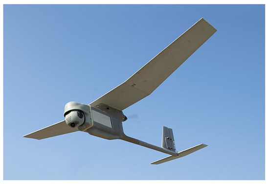
Figure 15.
Example fixed-wing SUAS (photo by A. Pena, US Air Force).
Equation (7) predicts range for an all-electric aircraft [34] as a function of the battery energy density (E), gravitational acceleration (g), total powertrain efficiency (), vehicle lift-to-drag ratio (), and the battery mass fraction (). As an example, we populate all the terms except the total efficiency with conservative static estimates for an SUAS like the Raven. We set E = 170 Wh/kg, g = 9.81 m/s, = 5, and = 0.3. Documentation for the military Raven SUAS is sparse, and the particular values we select are not as important as the modeling capabilities.
Our motor and controller models enable us to predict for different propeller speeds. The required inputs are propeller speed, propeller torque, system voltage, and the component specifications of the motor and controller. We prescribe a propeller speed range of 1000–3000 rev/min. We assume a constant mechanical power of 200 W, so the corresponding torque range is 1.9–0.7 N·m for the prescribed speed points. We also prescribe a voltage range of 12–24 V since voltage and rotational speed are closely linked in a motor [7]. We prescribe the specifications of the second motor in Table A1 and the controller specifications recommended in Section 3. Again, documentation for the Raven is sparse, and the particular values we assign for the model parameters are not as important as the high-level trends and insights that the models can deliver.
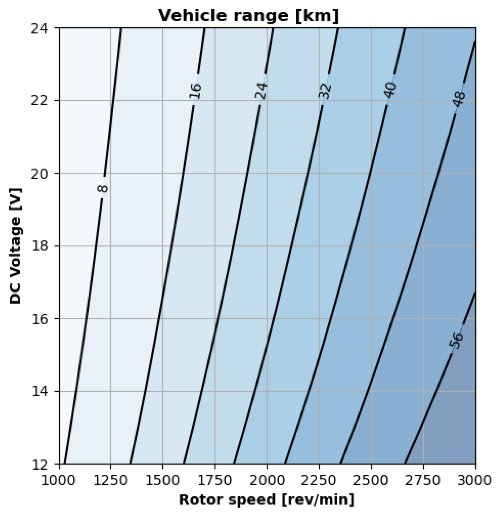
Figure 16 plots the range predicted using Equation (7) in combination with our integrated motor–controller model. The plot window is bounded by the prescribed voltage and propeller speed ranges. The contour lines mark the predicted range. At constant voltage, decreasing propeller speed decreases the overall range because of the same dynamics seen in the previous case study: harmonic losses. The motor controller must increasingly modulate (inhibit) the system voltage to achieve a lower propeller speed. The modulation introduces noise into the waveforms between the motor and controller, which generate heat and decrease overall efficiency. However, decreasing voltage alongside propeller speed can maintain the vehicle’s range. Directly decreasing the system voltage, such as with a different battery configuration, relieves the controller of the modulation burden.
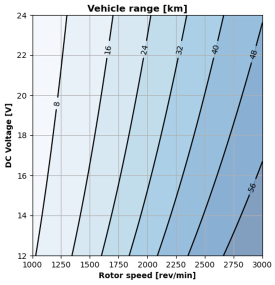
Figure 16.
Aircraft range predicted using motor and controller models.
These results are valuable because they shed light on the coupling between different sub-systems with minimal user input. Reducing propeller speed to reduce vehicle noise can also reduce the vehicle range if commensurate changes are not made to the vehicle’s bus voltage. A conceptual designer cannot attain such information as easily with other tools. The constant efficiency assumption does not inherently capture how changing propeller speed at constant mechanical power affects overall efficiency. The methods in the literature developed by Thurlbeck [17] and Gong [2] and the pre-built modules in proprietary tools like Simulink [16] require the designer to obtain certain model inputs experimentally, like the no-load current curve or the motor inductances, to populate the particular motor and controller models.
5. Discussion
5.1. Experimental Data
The experimental results show that a small electric UAS’s powertrain efficiency is far below the popular assumption of 90% efficiency. For example, the motor efficiency alone dips as low as 60% in Figure 6c. Assuming a 90% efficiency for the controller is reasonable, though not always true. The motor controller, which consists of solid-state electronics with no moving parts, dips below 90% efficiency in Figure 7d.
The experimental results motivate the need for aircraft designers to account for powertrain losses early in the design stage. Electrical power requirements increase by 40% as calculations shift from an ideal 90% powertrain efficiency to more realistic values between 60%–70% efficiency. The increased power requirement then significantly affects other parameters like battery size and aircraft weight.
The experimental results can also help aerospace researchers validate other electric powertrain or aerodynamics models. Researchers and practitioners can use the proposed instrumentation to capture other in-flight phenomena. For example, an instrumentation system with six-axis force sensors for each rotor can capture all six forces & moments to validate rotor aerodynamics models.
5.2. Analytical Models
Our models push the boundary without encumbering the user with esoteric input requirements. The motor, controller, and battery models can predict the respective components’ losses using a few readily available parameters listed in Section 3. The battery model, for example, works with even fewer inputs than the popular shepherd model [32].
Now, aircraft designers can simulate different powertrain configurations over the course of an entire mission. The proposed integrated model can predict a quadcopter’s mission performance in seconds. Winslow et al. had to experimentally test for this data over minutes and hours [6]. Moreover, the user does not need empirical data to initialize the models. The user only needs (1) component specifications easily found in datasheets and (2) high-level parameters like torque and rotational speed, which the user can derive from a vehicle dynamics module.
The results of the integrated powertrain validation suggest our models are better than higher-fidelity tools like Simulink or AMESim for power and efficiency analysis by vehicle designers. The latter tools require inputs like motor inductance and rotor inertia to predict the transient response of a motor with micro-second precision. Unfortunately, SUAS motor manufacturers do not publish these parameters, so a user must empirically measure these specifications for every motor they wish to evaluate. Our integrated models accurately predicted a battery’s dynamic discharge versus time within 5% of experimental values despite assuming instant motor response and steady-state losses. Moreover, our model used parameters that are published in SUAS motor datasheets.
5.3. Case Studies
The case studies encourage aerospace engineers to use the proposed models in all stages of aircraft development.
The weight reduction scenario in Case 1 shows how the models can help identify positive tradeoffs even for existing vehicles. Rather than physically swap motors to test performance, an engineer can analytically predict the current draw for different configurations using specifications commonly published for SUASs. Other models in the literature still require the user to characterize each motor experimentally to populate select inputs [2,16,17].
In Case 2, the models dynamically generate efficiency contours that show how only increasing the DC voltage can increase losses contrary to popular belief. Established motor design tools can also generate the requisite efficiency contours [35], but these methods are too complicated and computationally burdensome for aircraft designers.
The range analysis in Case 3 shows how the models can help predict ripple effects between aircraft systems in early design. Decreasing the nominal propeller speed can reduce acoustic signature, but aircraft designers should also adjust the nominal powertrain voltage in order to maintain the desired aircraft range.
5.4. Future Work
Peers may build upon this work by validating the component models for larger electric powertrains rated for manned vehicles (powertrains rated for tens of kilowatts). At small scales, aerospace researchers may expand the instrumentation of our quadcopter to measure the torque and rotational speed of all four propeller arms. Obtaining the torque for all four motors can improve the downstream battery voltage predictions. Instrumenting all four rotors with six-degree-of-freedom force sensors can also generate novel flight data for aerospace researchers to validate aerodynamic models.
6. Conclusions
Novel efficiency models were developed for the motor, motor controller, and battery found in small unmanned aerial systems. Novel efficiency data from a test stand validated the individual models. Novel torque data and battery data from a flying quadcopter validated the combined models. The integrated models predicted the quadcopter’s voltage discharge within 5% of experimental flight data for a 5+ min outdoor flight. Case studies showed how the models can inform vehicle-level design for a conceptual or existing small UAS. Practitioners can use the novel powertrain models to reduce development costs and timelines. Researchers can use the novel experimental data to validate other electric powertrain or aerodynamic models.
Author Contributions
Conceptualization, F.S. and M.B.; methodology, F.S.; software, F.S.; validation, F.S.; formal analysis, F.S. and M.B.; investigation, F.S.; resources, M.B.; data curation, F.S.; writing—original draft preparation, F.S.; writing—review and editing, M.B.; visualization, F.S. and M.B.; supervision, M.B.; project administration, M.B.; funding acquisition, M.B. All authors have read and agreed to the published version of the manuscript.
Funding
This research was sponsored by the Army Research Laboratory and was accomplished under Cooperative Agreement Number W911NF2020208. The views and conclusions contained in this document are those of the authors and should not be interpreted as representing the official policies, either expressed or implied, of the Army Research Laboratory or the U.S. Government. The U.S. Government is authorized to reproduce and distribute reprints for Government purposes notwithstanding any copyright notation herein.
Data Availability Statement
The data presented in this study are available in the article.
Acknowledgments
The authors thank Nathan Beals, Eric Spero, Matthew Johnson, and Dino Mitsingas for their support at Army Research Laboratory. The authors thank Nima Ershad and Matthew Gardner for their invaluable explanations and insights. The authors thank Dalton Chancellor and Tristan White for helping build the hover stand. The authors thank David Coleman, Noah Vanous, and Ian Voland for their help with the instrumented quadcopter. The authors also thank Noah for helping proofread earlier manuscript drafts.
Conflicts of Interest
The authors declare no conflict of interest.
Appendix A
Table A1 lists the motors tested on the test stand along with salient specifications for the motor model. All motors were paired with a Castle Creations HV Edge 60 A motor controller (also known as an electronic speed controller or ESC). All motors were sourced from KDE Direct. The tabulated model numbers omit the common “KDE” prefix for clarity.
Table A1.
Motors tested on test stand.
Table A1.
Motors tested on test stand.
| Model No. | Propeller Diameter | No. Blades | ||||
|---|---|---|---|---|---|---|
| (mN·m/A) | (A) | (m) | (in) | (cm) | (-) | |
| 2814XF-515 | 18.5 | 0.3 | 130 | 15.5 | 39.3 | 2 |
| 4215XF-465 | 20.5 | 0.7 | 52 | 15.5 | 39.3 | 3 |
| 5215XF-330 | 28.9 | 0.7 | 44 | 21.3 | 54.1 | 3 |
| 4012XF-400 | 23.9 | 0.3 | 78 | 15.5 | 39.3 | 2 |
Table A2 lists the batteries tested on the test stand along with their internal resistance. These were generic hobbyist lithium-polymer batteries sourced from a variety of vendors.
Table A2.
Batteries tested on test stand.
Table A2.
Batteries tested on test stand.
| Battery | Capacity | Series Cells | |
|---|---|---|---|
| (A·h) | (-) | (m) | |
| 1 | 0.6 | 3 | 17 |
| 2 | 2 | 3 | 13 |
| 3 | 1.8 | 3 | 22 |
References
- Nazarudeen, S.B.; Liscouët, J. State-of-the-Art and Directions for the Conceptual Design of Safety-Critical Unmanned and Autonomous Aerial Vehicles. In Proceedings of the 2021 IEEE International Conference on Autonomous Systems (ICAS), Montreal, QC, Canada, 11–13 August 2021; pp. 1–5. [Google Scholar] [CrossRef]
- Gong, A.; MacNeill, R.; Verstraete, D. Performance Testing and Modeling of a Brushless DC Motor, Electronic Speed Controller and Propeller for a Small UAV Application. In Proceedings of the 2018 Joint Propulsion Conference, Cincinnati, OH, USA, 9–11 July 2018. [Google Scholar] [CrossRef]
- Saemi, F.; Benedict, M.; Beals, N. Semi-Empirical Modeling of Group 1 UAS Electric Powertrains. In Proceedings of the Vertical Flight Society 75nd Annual Forum and Technology Display, Philadelphia, PA, USA, 13–16 May 2019. [Google Scholar] [CrossRef]
- Cheng, A.; Fisher, Z.; Gautier, R.; Cooksey, K.; Beals, N.; Mavris, D. A Model-Based Approach to the Automated Design of Micro-Autonomous Multirotor Vehicle Systems. In Proceedings of the American Helicopter Society 72nd Annual Forum and Technology Display, Palm Beach, FL, USA, 17–19 May 2016. [Google Scholar]
- Gong, A.; Maunder, H.; Verstraete, D. Development of an in-flight thrust measurement system for UAVs. In Proceedings of the 53rd AIAA/SAE/ASEE Joint Propulsion Conference, Atlanta, GA, USA, 10–12 July 2017; p. 5092. [Google Scholar] [CrossRef]
- Winslow, J.; Benedict, M.; Hrishikeshavan, V.; Chopra, I. Design, development, and flight testing of a high endurance micro quadrotor helicopter. Int. J. Micro Air Veh. 2016, 8, 155–169. [Google Scholar] [CrossRef]
- Hanselman, D.C. Brushless Permanent Magnet Motor Design; The Writers’ Collective: Cranston, RI, USA, 2003. [Google Scholar]
- KDE 10218XF-105 Technical Specifications. Available online: https://bit.ly/412Ggjw (accessed on 15 November 2023).
- EMRAX 188 Technical Data. Available online: https://bit.ly/3uxXMjh (accessed on 15 November 2023).
- Runco, C.; Benedict, M. Flight dynamics model identification of a meso-scale twin-cyclocopter in hover. Int. J. Micro Air Veh. 2023, 15, 17568293231206943. [Google Scholar] [CrossRef]
- Leishman, G.J. Principles of Helicopter Aerodynamics with CD Extra; Cambridge University Press: Cambridge, UK, 2006. [Google Scholar]
- Sridharan, A.; Govindarajan, B.; Chopra, I. A scalability study of the multirotor biplane tailsitter using conceptual sizing. J. Am. Helicopter Soc. 2020, 65, 1–18. [Google Scholar] [CrossRef]
- Vegh, J.M.; Botero, E.; Clark, M.; Smart, J.; Alonso, J.J. Current capabilities and challenges of NDARC and SUAVE for eVTOL aircraft design and analysis. In Proceedings of the 2019 AIAA/IEEE Electric Aircraft Technologies Symposium (EATS), Indianapolis, IN, USA, 22–24 August 2019; pp. 1–19. [Google Scholar] [CrossRef]
- Johnson, W. NDARC-NASA Design and Analysis of Rotorcraft. In Proceedings of the American Helicopter Society Aeromechanics Specialists’ Conference, San Francisco, CA, USA, 22–24 January 2015; Available online: https://ntrs.nasa.gov/citations/20110002948 (accessed on 7 July 2023).
- Rahman, S.; Hasanpour, S.; Khan, I.; Toliyat, H.A.; Hussain, H.A. Power Dense High-Speed Motor-Generator System for Powering Futuristic Unmanned Aircraft System (UAS). In Proceedings of the IECON 2022–48th Annual Conference of the IEEE Industrial Electronics Society, Brussels, Belgium, 17–20 October 2022; pp. 1–6. [Google Scholar] [CrossRef]
- Three-Winding Brushless DC Motor with Trapezoidal Flux Distribution. Available online: https://bit.ly/47SkmSa (accessed on 15 November 2023).
- Thurlbeck, A.P.; Cao, Y. Analysis and Modeling of UAV Power System Architectures. In Proceedings of the 2019 IEEE Transportation Electrification Conference and Expo (ITEC), Detroit, MI, USA, 19–21 June 2019; pp. 1–8. [Google Scholar] [CrossRef]
- Dehesa, D.; Menon, S.; Brown, S.; Hagen, C. Dynamic Analysis of a Series Hybrid–Electric Powertrain for an Unmanned Aerial Vehicle. J. Propuls. Power 2022, 38, 84–96. [Google Scholar] [CrossRef]
- Du, T.; Schulz, A.; Zhu, B.; Bickel, B.; Matusik, W. Computational Multicopter Design. ACM Trans. Graph. 2016, 35, 1–10. [Google Scholar] [CrossRef]
- Fletcher, J.W. Identification of UH-60 Stability Derivative Models in Hover from Flight Test Data. J. Am. Helicopter Soc. 1995, 40, 32–46. [Google Scholar] [CrossRef]
- Knowlton, A.E. Electric Power Metering: A Textbook of Practical Fundamentals; McGraw-Hill Book Company, Incorporated: New York, NY, USA, 1934. [Google Scholar]
- Saemi, F.; Dunston, O.; Benedict, M.; Mitsingas, C. In-flight Measurements and Validation of Electric Powertrain Models. In Proceedings of the Vertical Flight Society 79th Annual Forum and Technology Display, West Palm Beach, FL, USA, 16–18 May 2023. [Google Scholar]
- Mohan, N. Electric Machines and Drives: A First Course; Wiley: Hoboken, NJ, USA, 2012. [Google Scholar]
- Toliyat, H.A.; Kliman, G.B. Handbook of Electric Motors; CRC Press: Boca Raton, FL, USA, 2018. [Google Scholar] [CrossRef]
- Hart, D.W. Power Electronics; Tata McGraw-Hill Education: New York, NY, USA, 2011. [Google Scholar]
- Johnson, W.; Silva, C.; Solis, E. Concept vehicles for VTOL air taxi operations. In Proceedings of the AHS Specialists Conference on Aeromechanics Design for Transformative Vertical Flight, San Francisco, CA, USA, 16–18 January 2018; p. ARC-E-DAATN50731. Available online: https://ntrs.nasa.gov/citations/20180003381 (accessed on 7 July 2023).
- Hughes, A.; Drury, W. Electric Motors and Drives: Fundamentals, Types and Applications; Elsevier Ltd.: Newnes, NSW, Australia, 2013. [Google Scholar] [CrossRef]
- JETI MEZON EVO 85 OPTO. Available online: https://bit.ly/48aY7aD (accessed on 7 July 2023).
- Fairchild Semiconductors. 60 V LOGIC N-Channel MOSFET FQP30N06L Rev. A1. Available online: https://bit.ly/3usvhDC (accessed on 7 July 2023).
- Abu-Sharkh, S.; Doerffel, D. Rapid test and non-linear model characterisation of solid-state lithium-ion batteries. J. Power Sources 2004, 130, 266–274. [Google Scholar] [CrossRef]
- Chen, M.; Rincon-Mora, G. Accurate Electrical Battery Model Capable of Predicting Runtime and I–V Performance. IEEE Trans. Energy Convers. 2006, 21, 504–511. [Google Scholar] [CrossRef]
- Shepherd, C.M. Design of primary and secondary cells: II. An equation describing battery discharge. J. Electrochem. Soc. 1965, 112, 657. [Google Scholar] [CrossRef]
- Coleman, D.; Halder, A.; Saemi, F.; Runco, C.; Denton, H.; Lee, B.; Subramanian, V.; Greenwood, E.; Lakshminaryan, V.; Benedict, M. Development of “Aria” a Compact, Quiet Personal Electric Helicopter. J. Am. Helicopter Soc. 2023, 68, 42011–42024. [Google Scholar] [CrossRef]
- Hepperle, M. Electric Flight-Potential and Limitations. Available online: https://bit.ly/3usxDSY (accessed on 1 June 2023).
- Motor Design Limited. MotorCAD v14.1; Motor Design Limited: Wrexham, UK, 2021. [Google Scholar]


Disclaimer/Publisher’s Note: The statements, opinions and data contained in all publications are solely those of the individual author(s) and contributor(s) and not of MDPI and/or the editor(s). MDPI and/or the editor(s) disclaim responsibility for any injury to people or property resulting from any ideas, methods, instructions or products referred to in the content. |
© 2023 by the authors. Licensee MDPI, Basel, Switzerland. This article is an open access article distributed under the terms and conditions of the Creative Commons Attribution (CC BY) license (https://creativecommons.org/licenses/by/4.0/).