Abstract
The problem of maximizing the range of a propeller-driven aircraft in a level flight cruise is analyzed within the framework of optimal control. The specific fuel consumption and propeller efficiency of its propulsive system are characterized by functions of the velocity and engine power (full model), in contrast to previous works, where they were considered to be constant. To conduct the study, a notional Piper Cherokee PA-28 is selected as representative of light aircraft, defining both the airplane and mission features. Two simplified models are also derived: the Von Mises model, with constant specific fuel consumption and propeller efficiency, and the Parget and Ardema model, defined by constant specific fuel consumption and propeller efficiency depending on the velocity. The problem is solved numerically by means of a direct transcription method. Since the optimal problems of the Von Mises and Parget and Ardema models are singular, it is necessary to incorporate a regularization term. Such a numerical algorithm is validated against the analytical solution given by the Breguet formulation. In this context, the velocity and mass (state variables), the power throttle (control), and the best range are determined. The full model provides a maximum range of 1492 km. The differences between the Von Mises and Parget and Ardema models are about 24 km and 1 km, respectively. A non-optimal steady cruise is also analyzed, providing a significant reduction in the flight time, with a decrease of about 2% of the range. The evolution of the state variables and control in the steady cruise, however, separates from the full model. On the other hand, the Parget and Ardema model almost reproduces the full model results, leading to a clear image of the physics involved: the best range comes from maximizing the product of the propeller and aerodynamic efficiencies with respect to the velocity, which determines the optimal arc.
1. Introduction
Range is a key parameter in both the design and operation of an aircraft. The determination of the maximum, or best, range for a given amount of fuel is a problem that goes back to the early studies of flight mechanics in the first decades of the 20th century.
In many monographs (e.g., Miele [1], chapter 9; Hale [2], chapter 6; or Anderson [3], chapter 5), the procedure used to derive the maximum range of an aircraft belongs to the integral performance problems of flight mechanics (e.g., Miele [1], chapter 8). Another more general approach is based on formulating the maximum range as an optimal control problem. The reader can find a review of the first contributions in Bryson [4], as well as some subsequent representative research by Saucier et al. [5]. The main advantages of this framework are that it provides a greater generality and allows us to introduce different restrictions related to the aircfraft, the flight envelope, and the function to be optimized.
Logically, the price to be paid is that the derivation of the solution of the problem is much more involved. However, one of the reasons for the success of this formulation was the availability of powerful numerical methods of solution and computers at the end of the 1980s (e.g., Hargraves and Paris [6]). The main idea is to transform the original problem into a parameter optimization one (Morante et al. [7]), i.e., a nonlinear programming problem (NLP). A variety of methods exist in the literature and have been summarized in classical surveys by Betts [8], Rao [9], or Conway [10], or in more novel approaches, such as the theory of functional connections (TFC) (Mai and Mortari [11] and Leake et al. [12]), among others.
With these tools, complete scenarios have been addressed. To cite a few examples, they go from the first studies, such as that of Betts and Cramer [13], who considered the optimization of a commercial aircraft for different mission profiles, to more recent works that incorporate convective weather conditions into the dynamics of the flight (González–Arribas et al. [14]).
Other problems that can be tackled by means of optimal control methods are of a more fundamental nature. However, they provide interesting and sometimes unexpected solutions. An example of this is the case of the chattering, or oscillatory, cruise (e.g., Menon [15]). In a similar way, some situations concerning the maximum range of a cruise at constant altitude lead to singular control problems (e.g., Bell and Jacobson [16]).
Another example is Parget and Ardema [17], who studied the maximum range of an aircraft flying at constant altitude and heading, equipped with a turbojet or turbofan engine. The model of the aircraft was simple and assumed a parabolic drag polar, but the propulsive system incorporated the dependences of the thrust and the specific fuel consumption on the velocity. In contrast, simpler approaches take both as constant.
With such premises, the resulting optimal control is singular, and particular solutions must be employed. Parget and Ardema [17] implemented an indirect method, developing the Hamiltonian of the system and determining the singular arc through the Kelley condition (Kelley et al. [18]).
Later, this study was extended by different works, for example, Rivas and Valenzuela [19] and Franco and Rivas [20], or approached from other perspectives, such as the Green theorem (Ardema and Asuncion [21]).
All these studies considered turbojets, with the exception of Ardema and Asuncion [21], who also addressed other propulsive systems but with simple models and giving very few details, except for the turbojet case. For example, they modeled a reciprocating engine–propeller aircraft by constant specific fuel consumption and propeller efficiency (the ideal airplane by Von Mises [22], chapter XV), providing only the algebraic expression of the maximum range and endurance.
Indeed, those conditions of the propulsive system of reciprocating engine–propeller aircraft are very common in works on performance research (e.g., Cavcar and CavCar [23]), which seldom employ more realistic models, although there are some exceptions, such as Lowry [24], Tulapurkara et al. [25], and Donateo and Totaro [26]. Furthermore, to our knowledge, most of those studies were worked out as integral performance problems.
More recent studies of reciprocating engine–propeller aircraft include the performance analysis of small aircraft considering propeller effects, such as that of Rostami et al. [27]. Other works are more focused on examining new technologies and aerospace platforms, such as characterizing the aerodynamics of unnamed aerial vehicles (UAV) (e.g., Bergmann et al. [28]) or determining the effects of hybrid or electric systems on the performance of light aircraft, for example, Bravo et al. [29].
Here, we aim to extend the problem of the maximum range posed by Parget and Ardema [17] to a reciprocating engine–propeller aircraft. The research is conducted for a notional Piper Cherokee PA-28 as a representative model of a light aircraft.
However, in contrast to other analyses, our characterization of the propulsive system, consisting of the propeller and the piston engine, is more realistic. It takes into account potential dependences on the velocity and the power of both the propeller efficiency and the specific fuel consumption.
Complementary to the former model of the propulsive system, the full model, we develop two simplified models: the classical approach, with a constant specific fuel consumption and propeller efficiency, i.e., the Von Mises model, and another case with constant specific fuel consumption and propeller efficiency depending on the velocity. This last model stems from an analogy with the model considered by Parget and Ardema [17] for turbojets; hence, we call it the Parget and Ardema model, and from now on, it is referred to as the PA model.
As in Parget and Ardema [17], the approach is derived from the optimal control perspective. The complexities in the modeling, however, make it necessary to find a solution by numerical means.
For that purpose, we implement a simple, quick, and reasonably accurate algorithm based on a direct transcription method (e.g., Betts [30]). Nevertheless, the optimal problems corresponding to the Von Mises and PA models are singular, so it is necessary to enhance such an algorithm by adding a regularization term (e.g., Bell and Jacobson [16]).
With these tools, we solve the problem of the maximum cruise range for those three models; that is to say, we determine the evolution of the state variables: velocity and mass, the control variable: power setting, and the best range, also detailing the characteristics of the optimal flights and comparing them with a typical constant speed flight program (steady cruise). This methodology constitutes a new approach that has not been presented in the literature, as it combines a realistic model for the propulsive system, beyond taking both constant specific fuel consumption and propeller efficiency, with a transcription numerical method including a regularization term. It offers a valuable solution to compute optimal flights of light aircraft or other similar platforms, such as some unmanned air vehicles (UAV) (e.g., Zheng et al. [31] or Li et al. [32]).
The structure of the paper is as follows. In Section 2, we provide the equations of motion of the flight and outline the general characteristics of the propulsive system of a reciprocating engine–propeller aircraft. That leads to formulating the maximum cruise range as an optimal control problem with its functional to be optimized, as well as the differential equations and constraints.
Next, in Section 3, we develop the particular model of the propulsive system (full model) for a notional Piper Cherokee PA-28. Additionally, we also construct two simplified characterizations (the Von Mises and PA models). The numerical algorithm employed in the resolution is described in Section 4. After briefly reviewing the main steps of the implementation of a direct transcription method, we complete it by adding a regularization term. That term is necessary to obtain the solutions of singular problems.
In Section 5, we include the results of our research. First, our numerical algorithm is validated with respect to the Breguet analytical solution. After that, we present the results for the three models of the propulsive system and for the constant speed program, detailing the characteristics of the optimal flights. We pay special attention to the comparison between the full and PA models since the PA model is a very good approximation of the full model in the cruise flight and is also easier to analyze. Finally, we draw some conclusions regarding our contribution in Section 6.
2. Cruise Conditions and Propulsion System
The functional to be optimized is the range of an aircraft in cruise flight at constant altitude, also referred to as level flight, e.g., how the airplane must be controlled in such flight conditions to cover the maximum distance for a given amount of fuel.
This situation is the first to be addressed for integral performance problems in classical texts of flight mechanics (e.g., Von Mises [22], chapter XVI). The reason is that it is commonly the dominant phase of the flight; that is why it plays a key role in the conceptual design of an airplane (e.g., Anderson [3], chapter 7).
First, it is necessary to pose the optimal control problem to be discussed. It requires to consider the dynamics of level flight, as well as specifying some features regarding the propulsion system of the aircraft.
2.1. Flight Dynamics
The dynamics of the problem are presented in many studies of flight mechanics (e.g., Miele [1], chapter 4). We employ the formulation given by Pargett and Ardema [17]. Since we are considering a reciprocating engine–propeller aircraft, such equations are best formulated in terms of power instead of thrust (e.g., Anderson [3], chapter 5)
In these expressions, V is the aircraft velocity, i.e., true airspeed, and m is its mass; and are, respectively, the available and the required powers obtained from the thrust T given by the propeller and the drag force D; L is the lift force; is the fuel flow rate; and g the gravitational acceleration, taken as m/s2 from the International Standard Atmosphere (ISA). It is assumed that Equation (1) is compatible with the aerodynamic characteristics of the aircraft, entailing, for example, that the required lift can be reached.
Additionally, a parabolic drag polar defining the relation between the drag and lift forces (e.g., Anderson [3], chapter 2) is considered as follows
with
where is the air density given by the constant cruise altitude, considering ISA conditions; S the reference area of the airplane; the zero-lift drag coefficient and K the induced drag one.
The range is given by
with the flight taking place in the time interval . The state variables V and m, both functions of time t, are subject to the following inequalities (bounds and boundary conditions):
The constrains of the velocity are related to the flight envelope of the aircraft: the minimum is imposed by the stall restrictions, while the maximum is set by the structural limitations (e.g., Ruijgrok [33], chapter 10).
In the case of the mass, it decreases from its initial value in to the final one in , when the amount of fuel has been burned out. It also provides two boundary conditions
with being the mass of the aircraft fully equipped plus the payload, as well as the reserve fuel, if any.
2.2. Propulsion System Characterization
In contrast to a relatively simple jet engine, which is governed by a single control parameter, the thrust, the situation for the combination of the propeller and reciprocating engine is more complex.
The available power introduced in Equation (1) is given by the product of the propeller, or propulsive, efficiency and the power P delivered by the engine, e.g., shaft brake power (e.g., Ruijgrok [33], chapter 6)
The propeller efficiency can be expressed in terms of the dimensionless thrust and power coefficients. Such coefficients are associated, respectively, with the thrust and power generated by the propeller (e.g., Ruijgrok [33], chapter 7 or Torenbeek [34], chapter 6)
where is the number of revolutions of the propeller and its diameter. Both and are mainly functions of the blade angle at 75% of the radial distance, , and the advance ratio J
In terms of these variables, the propeller efficiency can be written as follows
In turn, given the atmospheric conditions, the power of the engine P is a function of the power throttle parameter , the rotational speed of the engine n is measured in revolutions per second, and the fuel–air mixture is (e.g., Lowry [24], chapter 5). Additionally, despite being usually negligible, there is also a dependence on velocity, e.g., ram effect (e.g., Anderson [3], chapter 5). So, initially, one can assume .
The fuel flow rate introduced in Equation (1) is expressed as
where C is the specific fuel consumption, which is the mass of fuel burned per unit of time and engine power. It is important to note that sometimes the specific fuel consumption refers to the weight of fuel (e.g., Ruijgrok [33], chapter 6), not its mass, being equivalent to our .
In a similar way to P, for a given atmosphere, the flow rate can also be viewed as a function of , n, and . Additionally, as derived from the performance charts of different engines, e.g., Lycoming [35], it is extended to V too. That dependence is translated into the specific fuel consumption, which initially could be written in the form .
Control Function
The available controls for this propulsive system, including both the propeller and the engine, depending on whether the blade angle can be controlled or not (e.g., Lowry [24], chapter 5).
For a fixed-pitch propeller, the controls are limited to the power throttle and the mixture control, whereas for variable-pitch propellers of constant speed (e.g., Torenbeek [34], chapter 6), it is also possible to control the propeller rotational speed. Hence, in the most general situation, the combination of a propeller and reciprocating engine has three controls, corresponding to , n, and .
However, within the scope of this research, we will just consider, as in most studies of flight mechanics, the power throttle. In particular, we will assume that the pilot fixes the mixture and the revolutions of the constant speed propeller, which equals those of the engine, i.e., . So, the power required by the propeller is always equal to that provided by the engine (e.g., Ruijgrok [33], chapter 7 or Torenbeek [34], chapter 6), i.e., .
Under such conditions, and . Hence, from Equations (8) and (10), we know that
providing . So, the propulsive efficiency and the available power, Equation (7), are also functions of V and P, i.e., and .
Therefore, with our assumptions, a cruise flight at constant altitude is only controlled by a scalar function, the power throttle . We can define (e.g., Pargett and Ardema [17]) an expression relating it with the engine power of the form
which controls the power generated by the reciprocating engine from a minimum value—it is not relevant for our purposes to fix a particular minimum value for compatible with the level flight conditions, since it will automatically be considered in the optimization process. Hence, the minimum possible value of the power is set to 0—to a maximum , which is a function of V, available at the given atmospheric, rotational speed, and mixture conditions.
In this situation, the power throttle is the control function with
or, misusing language, the engine power could alternatively be referred to as the control with
2.3. Optimal Control Problem for Cruise Maximum Range
Considering former developments, the optimal control problem to obtain the maximum range of an aircraft on the condition of cruise at constant altitude can be formulated as finding the control and the final time to minimize the functional
subject to the differential equations—the practical resolution of the equations benefits from considering dimensionless variables with a proper scaling (e.g., Betts [30], chapter 1), which we will introduce it when numerically solving the problem in Section 4—
with the simple bounds and boundary conditions being
In contrast to mass, there are no boundary conditions for velocity, i.e., their particular values are not fixed in the initial and final times.
Such equations must be supplemented with data specifying the mission (level flight) and aircraft features, including the characteristics of its propulsive system through—according to the notation introduced in Equation (15) the dependence of P on V, which comes from that of —, , and
3. Reciprocating Engine Light Aircraft: Piper Cherokee PA-28 Full and Simplified Models
For the calculations of the maximum cruise range, we have chosen an airplane of the Piper Cherokee family to perform a given level flight. This choice was mainly motivated by it being a good representative of a light aircraft with a propeller and reciprocating engine. The proposed methodology can be extended to other situations in a similar way.
In this context, the numerical solution of the optimization problem requires the characterization of the cruise mission and the reciprocating engine–propeller aircraft under consideration. From the formulation given in Equations (16)–(18), it entails that the following groups of data must be provided:
- Mission parameters (M): These define the requirements of the level flight, such as the altitude, the amount of fuel, the mixture conditions, and the rotational speed. So, it is necessary to specify h, , , and . For the sake of simplicity, we assume that the flight takes place under ISA conditions, which allows us to obtain the pressure, density, and temperature from h (if needed).
- Aircraft and propulsion system constants (AP): These are related to geometry, aerodynamics, structural masses, and the operational limits of both the airframe and the propulsion system. The involved quantities are S, , K, , , , , and .
- Propulsion system performance functional model (PFM): This describes the performance of the reciprocating engine and the propeller by providing the functions , , and .
Next, we present the data and functional models corresponding to a notional Piper Cherokee PA-28. It is a reasonably well-documented single reciprocating-engine aircraft, as shown in Figure 1, which similar to the PA-28-180 model but equipped with the variable-pitch propeller of the PA-28R-180 model.
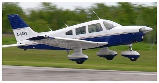
Figure 1.
Three-dimensional view of the Piper Cherokee PA-28 [36].
3.1. Piper Cherokee PA-28 and Level Flight Conditions
The public information necessary to characterize—although not for arbitrary flight conditions—our propeller-driven notional Piper Cherokee PA-28 was obtained from different sources.
Namely, the features of the aircraft were granted from the Aircraft Owner’s Handbook [37], the FAA type certificate data sheet [38], and McCormick [39]. With respect to the propulsive system, it was modeled through the performance charts given in the Lycoming operator’s manual [35] for the mounted Lycoming O-360-A engine, as well as the ones of the constant speed propeller Hartzell HC-C2YK-1/7666A-O provided by McCormick ([39], chapter 6). Other studies [25,26] have also used these sources to model the propulsive system of a Piper Cherokee PA-28 for a fixed pitch propeller. Its functional dependences are simpler than those considered here for a constant velocity propeller.
From these data and after establishing some common mission parameters for this type of light airplanes, all the values of the first and second groups, that is, the mission parameters (level flight) and the aircraft and propulsion system constants, can be obtained or estimated almost directly. They are all presented in Table 1.

Table 1.
Adopted data set for the Piper Cherokee PA-28 corresponding to the mission parameters (M) and the aircraft and propulsion system constants (AP).
For the third group, propulsion system performance, the situation is more challenging because it is necessary to derive a functional model for , , and from the engine and propeller charts. This task will be discussed in the following subsections, where some simpler functional models for both the engine and the propeller will also be obtained.
3.2. Reciprocating Engine Model
In the case of the O-360-A engine (Lycoming operator’s manual [35], figures 3–17), a chart of the sea level performance for both the engine power and the fuel flow rate as functions of the manifold absolute pressure (MAP), which can be related to the power throttle (for our purposes, the engine power P can be related to MAP by an affine relationship of the form , both in kW), is provided for different revolutions. Additionally, an adjacent plot is employed to correct such values for different altitudes, e.g., a non-turbocharged engine, and deviations from the corresponding ISA temperature. The procedure for determining the values from the charts is explained, for example, in McCormick ([39], chapter 6) and Ruijgrok ([33], chapter 6).
The curves, which include additional information, are constructed for very particular conditions like maximum power mixture. Moreover, since they are obtained from bench testing, they provide no information about the influence of V on P and . However, considering the typical velocities of a light airplane, the ram effect is negligible (e.g., Hale [2], chapter 2, or Anderson [3], chapter 5), so the influence of V on P and can be ignored; hence, this is also the case for C. In such circumstances, under the conditions given in Table 1 for altitude and rotational speed, we can compute directly with a value of kW.
To obtain a functional model for the flow rate, we construct the fitting polynomial in a (linear) least-square sense to all the data in the entire range covered by the chart—the values of the chart (Lycoming operator’s manual [35], figures 3–17), given in terms of P, are kW for the minimum and and kW for the maximum. Such an approach avoids some flaws encountered by numerical optimization if a polynomial interpolation, or extrapolation in some cases, is used (see Betts [30], chapter 6). It is be possible to use higher order polynomials to ensure continuous differentiability, e.g., splines, but they also present some drawbacks like the appearance of spurious oscillations (e.g., Betts [30], chapter 6).
In this way, we fitted the 27 points using a polynomial in P. It turns out to be a quadratic polynomial in P, with a coefficient of determination , of the following form (all the fitting functions presented in this work are constructed to introduce the variables in the SI units except the power, which is always in kW)
The resulting parabola degenerates in an almost straight line, as it is commonly found in this kind of chart (e.g., Lowry [24], chapter 5). From this, the desired functional expression of C is obtained as follows
3.3. Propeller Model
The properties of the constant speed propeller Hartzell HC-C2YK-1/7666A-O are presented by McCormick ([39], chapter 6, figures 6.19 and 6.20) through two charts. In the first one, the propulsive efficiency is represented with respect to the advance ratio J for different values of the blade angle . The second one is similar, but it considers the power coefficient instead of . The way to obtain as a function of and J is detailed, for instance, in McCormick ([39], chapter 6) or Ruijgrok ([33], chapter 7), and uses as a proxy.
In this way, as in the case of the engine, to catch the functional dependence of the function , we derive the fitting polynomial in V and P, linear least squares, to the 142 points considered, resulting in a cubic polynomial of the following form
After that, we repeat the same procedure for the chart of with respect to J, obtaining 174 points of the form , where is the associated value to within the interval and , , …, . From these tabular data, we compute the least square fitting polynomial in V and . It is also a cubic polynomial given by
In this way we obtain the desired expression for through and . The respective data points and the fitting surfaces are plotted in Figure 2.
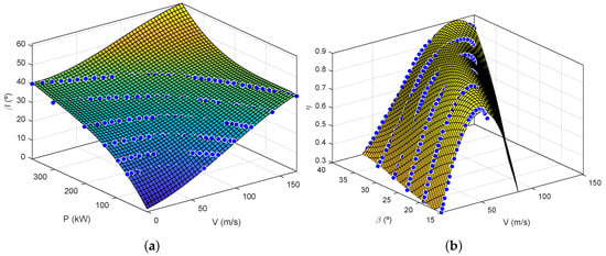
Figure 2.
Surfaces generated with the fitting polynomials (a) for blade angle (third degree in P and V with a coefficient of determination ) and (b) the propulsive efficiency (third degree in and V with coefficient of determination ) derived from the available data points of the constant speed propeller Hartzell HC-C2YK-1/7666A-O [39].
3.4. Simplified Models
The former Equations (20)–(22) define the performance of the propulsion system of our Piper Cherokee PA-28 numerically. The expressions involved, even being of polynomial form, entail a certain degree of complexity, especially for the propulsive efficiency. Hence, it is interesting to introduce other suitable simplified models.
3.4.1. Von Mises Model
The first simplified model considered is referred to as the ideal airplane (e.g., Von Mises [22], chapter XV) and consists of assuming that is independent of velocity for a given mass and altitude. Typically, such a condition is achieved by imposing that both C and are also constant.
This is the common way of dealing analytically with the problem of maximum range in cruise flight (e.g., Von Mises [22], chapter XVI; Miele [1], chapter 9; Hale [2], chapter 6). Along with some other dynamic simplifications, it allows the range problem to be tackled with the ordinary theory of maxima and minima, which leads to the commonly named Breguet range equation (e.g., Von Mises [22], chapter XVI)—for a discussion about to what extent it is appropriate to use the denomination “Breguet equation or formula” see Cavcar [41]).
Under such conditions, the maximum range in a cruise flight at constant altitude for a reciprocating-propeller airplane is given by (e.g., Miele [1], chapter 9)
entailing that the angle of attack must be kept constant during the flight, with a value that provides the maximum aerodynamic efficiency, lift-to-drag ratio, , which for a parabolic polar is given by (e.g., Miele [1], chapter 9, and Equation (3))
To obtain the mentioned constant values of C and for the Von Mises model of the Piper Cherokee PA-28, we start from Equations (20) and (22) of the full model and fix some representative values of the velocity V and the available power . In particular, following Miele ([1], chapter 9), we introduce the following parameters:
The reference velocity is defined by the condition of providing the minimum drag with , where the reference available power is obtained from the reference thrust that equals the minimum drag when .
In Equation (25) the mass enters into the definition of and that, in our case, changes with time in the interval . However, we checked that such variation does not significantly affect our results, since is about of (Table 1). So, an averaged value of is taken as a representative mass of the entire level flight.
Under those conditions, we obtained m/s and kW. Then, substituting these values in Equations (21) and (22) leads the solution of , which allows us to compute through Equation (20).
By doing so, the functional model of the propulsion system (engine plus propeller) for the Von Mises model of the Piper Cherokee PA-28 is characterized by the following constants:
3.4.2. Pargett and Ardema Model
A second simplified model can be constructed by allowing some dependence of and C on the state variables or the control. In the case of the specific fuel consumption given by Equation (20), its dependence with engine power P is quite flat. Hence, it is reasonable to keep it constant, taking the same value as the one used for the Von Mises model.
We could proceed in the same way with the propeller efficiency , so that it is just a function of velocity by taking . However, a more precise procedure that takes into account the variation of P during the level flight will be implemented. In particular, we will follow an analogous methodology to the one applied in Pargett and Ardema [17], where the authors generated a simplified model of the fuel specific consumption, i.e., , of the jet engine by imposing that the thrust matches the drag of the aircraft in terms of speed, a condition representative of level flight (Pargett and Ardema [17]). In this way, the specific fuel consumption is transformed into a function of velocity only, removing the dependence on the thrust throttle, which was the control function of the problem.
In our case, we face a similar situation, but with the propulsive efficiency instead of the specific fuel consumption of the jet engine. Taking this as a reference, we build a new functional model, with subscript PA from Pargett and Ardema, based on the condition that in level flight, the available power matches the required power . It is important to note that, as in Equation (25), it is necessary to define the value of the mass m, which changes with time—Pargett and Ardema [17] did not provide any information about this point. However, its particular value does not influence our results in a noticeable way; hence, we took , as in the case of the Von Mises model.
With this procedure, we derived 174 points of the form . Proceeding in the same way as in former cases, we computed the least square fitting polynomial in V. It resulted in a fifth degree polynomial of the following form:
Thus, the propeller efficiency is given by Equation (27) and the constant value of the specific fuel consumption:
which characterizes the functional model of the propulsion system (engine plus propeller) for the Pargett and Ardema model of the Piper Cherokee PA-28.
4. Numerical Solution Method
According to the results of Section 3, the optimal control problem for the maximum cruise range will be solved for three functional models of the propulsion system of the Piper Cherokee PA-28, having a quite different nature compared to the optimal control problems point of view.
On the one hand, the specific fuel consumption C for the Von Mises and PA models is constant, while the propulsive efficiency does not depend on P. Under these circumstances, the optimal control problems for such models, the simplest ones from a propulsion perspective, are singular, which makes their resolution more cumbersome.
On the other hand, since for the full model both C and are functions of P, the optimal problem turns out to be, in principle, regular.
Keeping in mind these considerations, one of the most versatile methods to obtain a solution for the three cases is to employ a numerical algorithm based on a direct transcription formulation (e.g., Betts [30], chapter 4) but adapted to solve singular problems through a regularization term. It allows us to tackle the singular and regular problems arising from our aircraft models with the same technique and in an almost automatic way.
4.1. Direct Transcription Method
Direct transcription methods, also referred to as collocation methods, transform the optimal control problem into a parameter optimization problem. That is to say, both the state and control functions are discretized into a set of values that stem from evaluating these functions at different times in . Therefore, the original problem is transcribed into a parameter optimization problem (e.g., Hargraves and Paris [6]). Such a parameter problem is generally non-linear and its optimization is subject to different algebraic constrains and bounds in the form of equalities or inequalities, resulting in a nonlinear programming problem (NLP).
So, it is first necessary to divide the time interval into N subintervals, leading to nodes, i.e., mess or grid points. With that aim, the given values are defined as
in such a way that
and the separation between the nodes, , turn out to be
Since the final time is unknown in our problem, is also a variable to be determined.
The evaluation of the state and control functions at each node leads to and parameters, respectively, defined as
So, the parameter matrix, NLP variables, to be obtained through parameter optimization is given by the unknowns
The substitution of Equations (30) and (32) into simple bounds, path constraints, and boundary constrains leads to algebraic inequality constrains of the following form
where to simplify the notation, the simple bounds have been incorporated as additional components of .
In order to discretize both the differential equations that define the dynamics of the system and the functional to be optimized, different schemes can be applied such as trapezoidal, Hermite–Simpson, etc., as described in the literature (e.g., Rao [9]; Conway [10]; Betts [30], chapter 3). In this way, for the first ones, another set of constraints needs to be introduced in addition to Equation (34) for the NLP problem, which can be written in the form of a general inequality constrain as
where represents the so-called N defects (Betts [30], chapter 3), with .
In the case of the functional to be minimized, it also needs to be discretized in a similar way, which turns the original functional into a function of several variables in the parameter matrix , i.e., into the function .
Therefore, summarizing Equations (34) and (35) and , the original optimal control problem has been transcribed into an NLP one formulated as follows
From this point, the numerical solution is computed by solving the resulting NLP (Equation (36)), which is sparse, and assessing the accuracy of the approximation through a mesh-refinement (e.g., Betts [30], chapter 4).
4.2. Regularization Term
The direct application of the former numerical transcription algorithm leads to difficulties in the solution of the control function for singular problems. They manifest in the form of spurious oscillations of the control (e.g., Betts [30], chapter 4, or Schwartz [42], chapter 4).
One way to deal with those difficulties, which is consistent with the formulation of direct methods, is to consider regularization. Basically, it consists of adding a term, , to the functional that eliminates the singularity of the problem, but without affecting the optimal solution (e.g., Bell and Jacobson ([16]; chapter 5).
In particular, we will adopt the form of the regularization term proposed by Schwartz ([42], chapter 4). In contrast to other classical regularizations (e.g., Jacobson et al. [43] or Pager and Rao [44]), such formulation does not exhibit numerical instabilities that appear in the classical approaches when using gradient-based algorithms to solve the NLP (Dadebo et al. [45]). In the work by Schwartz [42], the reader will be able to find the mathematical demonstrations that establish the convergence of that type of regularization.
For the sake of convenience, the notation of Schwartz [42] is adapted to the one employed in this manuscript. Specifically, we will introduce a regularization term, particularized to the case of having just a scalar control function, of the following form
where
The numerical parameter is fixed by the user from a trade off between skipping the singular nature of the problem, larger values of , and not altering its optimal solution, smaller values of . Since, in general, the scaling of states and controls is different, such small or large values are defined in relation to the ratio.
The numerical direct transcription formulation including the regularization term described in the previous paragraphs has been implemented in MATLAB for the trapezoidal and Hermite–Simpson schemes, with mesh-refinement accuracy control [30]. As an NLP solver, we used SNOPT (Gill et al. [46]). Other choices are possible, but sequential quadratic programming (SQP)-based methods have, in general, better performance (e.g., Betts [30], chapter 4).
We validated our algorithm, always with the regularization term included, with a variety of well-known optimal control problems available in the literature. We obtained proper results with reasonable accuracy (always below 1% of relative error) for the performance index, the state variables, and the control.
For example, that was the case obtaining solutions for regular problems, such as the space-shuttle re-entry trajectory by Betts ([30], chapter 6, example 6.1), for singular scenarios such as the Goddard rocket ascent problem (e.g., Betts [30], chapter 4, example 4.9), and also for bang bang problems, such as the Rayleigh one (Silva and Trélat [47], example B).
Additionally, we employed the previously defined Von Mises model to validate our algorithm, discussing it in detail in Section 5.2 once the particular setup of the numerical method necessary to solve this problem has been defined. It is performed comparing the results with those given by the analytical Breguet formulation, showing relative differences below 0.6% in absolute values between the analytical and numerical solutions.
5. Results
In this section, the numerical results that determine the maximum cruise range are presented. First, we outline the particular setup employed and validate the numerical algorithm with the Breguet analytical formulation. After that, we obtain and discuss the solutions of the cruise maximum range for the three functional models of the propulsion system of the Piper Cherokee PA-28 considered in the study: Von Mises, PA, and full models.
5.1. Setup of the Numerical Method
The particular implementation of the former framework to solve the problem of maximum cruise range needs to be described to define the baseline configuration of our numerical method.
First, before applying the numerical direct transcription formulation with the regularization, it is convenient to facilitate proper scaling of the state variables, the control, the time, and the range so that they have a similar order of magnitude in the evolution of the system. As it is well-known, good scaling makes it easier to obtain the solution of the NLP (e.g., Betts [30], chapters 1 and 4). Such transformations allow us to reformulate the optimal control problem in terms of the non-dimensional variables, where the interval becomes . The reference parameters employed to obtain the non-dimensional variables are .
In the case of the initial guess to start the iterations of the NLP, after different trials, we finally employed constant values equal to 1 for the non-dimensional variables at each node, as it was observed that convergence was not problematic.
We also carried out several tests employing both the trapezoidal and Hermite–Simpson schemes for the discretization. All the computations encountered the same difficulty: the unknowns in the first and final nodes, especially the dimensionless velocity, presented large variations. However, we observed that when fixing arbitrary values for the velocity within their bounds for and , those oscillations disappeared. So, we concluded that such situation was due to the lack of boundary conditions for the velocity in our optimal control problem. Hence, for this problem, the absence of those conditions led to several possible NLP solutions for the velocity in the initial and final nodes, compatible with small changes in .
A way to circumvent that difficulty in this particular case was to introduce an additional kinematic constraint that limits the variation of the velocity rate, i.e., (similar to Betts [30], chapter 6, example 6.3). Once that flaw was solved, our results showed that within the accuracy required for our problem, of the order of 1% in relative terms for the performance index, the state variables, and the control, discretization based on the trapezoidal method with a linear interpolant for the control provided satisfactory results. In addition, mesh refinement did not introduce significant enhancement, likely due to the fact that for this problem both the evolution of the state variables and the control are relatively smooth.
In view of these results, and with the aim of implementing the simplest algorithm compatible with our accuracy demands, we fixedm as a basic setup, a trapezoidal discretization with 60 equi-distributed subintervals in , 61 nodes, starting the iteration of the NLP from the value 1 for all the unknowns (we have a total of 184 unknowns). With respect to the regularization term, we fixed the value , while for the velocity kinematic constraint, a non-dimensional was imposed.
5.2. The Von Mises Model: Validation of the Numerical Solution
To validate the algorithm, the results of the Von Mises model—the Von Mises model could be solved as in Pargett and Ardema [17], obtaining an analytical solution, essentially equivalent to that of the Breguet formulation—are compared to the corresponding analytical solution, given by the Breguet formulas. Both approaches differ in the consideration of the inertial terms, which are not included in the Breguet formulation (e.g., Miele [1]), but their contribution to the solution is negligible. Hence, the comparison allows us to determine the validity of our numerical approach.
5.2.1. Results and Discussion
For the analytical solution of Breguet (Anderson [3], chapter 5), in addition to the Equation (23) determining the range, the evolution of the state variables is given by
As shown by Figure 3, where the time evolution of the state variables and the control are displayed, the numerical solution of the problem employing a transcription method with regularization shows very good agreement with the analytical one. In fact, the differences in the range and time of flight are of the order of 19 m and s, leading to relative errors, in absolute value, of about . This is also the case for the evolution of the velocity, mass, and power during the flight displayed in Figure 3 (red curves), which practically overlaps with the analytical results.
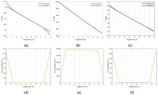
Figure 3.
In the upper panels, we show the time evolution of (a) V, (b) m, and (c) P during the optimal cruise for the Von Mises model: the blue line represents the analytical results, while the red line refers to the numerical ones. In the bottom panels, we display the relative errors of the numerical solution with respect to the analytical solution in percentage terms of (d) V, (e) m, and (f) P.
Larger differences were found for the velocity, and to a lesser extent for the power, at the beginning and the end of the flight. Such a circumstance is likely to be related to the lack of initial and final conditions for the velocity, as we pointed our in the previous section. In contrast, the differences of the mass, with fixed initial and final values, are more pronounced in the middle of the flight.
In any case, the relative differences between numerical and analytical solutions (Figure 3d–f) are very small during the cruise. Even in the worst situations, at the beginning and end of the flight, they are almost below .
The analytical solution is recovered, which proves the validity of the method for solving the optimal control problem under consideration.
5.2.2. Effect of the Regularization Term
The regularization term has a key role in our algorithm since the Von Mises model leads to a singular problem. In Figure 4, we present the time evolution of the power for different values of the regularization term using , respectively.
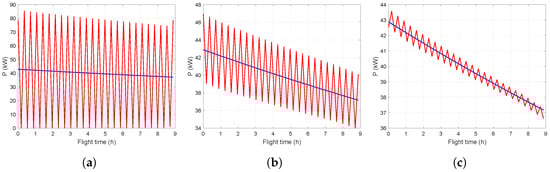
Figure 4.
Evolution of the control P during the optimal cruise flight in the Von Mises model, a singular control problem, for different values of in the regularization term (Equation (37)): (a) , (b) , and (c) .
It can be seen that the direct formulation of the optimal singular control problem with the numerical transcription method (Figure 4a) leads to oscillations in the control, with relative errors in some points of about . Such oscillations are a numerical artifact, not chattering phenomena (e.g., Zelikin & Borisov [48], chapter 1), since the real optimal control determined analytically is smooth, as shown in blue in Figure 4. When introducing a regularization term , the oscillations progressively damp out as the values of are increased (Figure 4b,c) until they are eliminated, as shown in Figure 3c with (basic setup).
Although the inclusion of is essential to describe the right evolution of P, and to a lesser extent of V and m, its effect on minimizing the range must be residual in order not to alter the nature of the optimal problem under consideration. Indeed this is the case, as shown by quite small relative differences with respect to the final optimal values of the range and the flight time, which never exceed .
Therefore, from the comparisons with the analytical solutions for the Von Mises model, we can conclude that our numerical algorithm based on a transcription method with a regularization term works properly to obtain a solution of this kind of optimal problems, singular or not.
5.3. Cruise Maximum Range for the Piper Cherokee PA-28: Comparison of Von Mises, PA, and Full Models
Apart from the Von Mises model, we introduced the full and the PA models in Section 3. So, it is expedient to compare the optimal arcs for such scenarios.
In addition to those models, from which an optimal arc maximizing the cruise range is computed, we also consider in our discussion a non-optimal cruise of constant speed associated to the full model, FullV=cte. That constant speed is larger than the typical best range velocity, which is relatively low, and is determined in the aircraft handbook, where such cruise recommended airspeed is related to the density altitude and the engine rpm under particular conditions. This kind of constant velocity flight program is common for propeller-driven light aircrafts because of the reduction in the time of flight, which is often more important than fuel savings for these platforms (e.g., Hale [2], chapter 6).
As a representative value of the constant velocity, we have taken m/s considering the characteristics of the mission (Table 1) and the information of the Aircraft Owner’s Handbook [37] for our particular airplane. It corresponds roughly to flying at about 60–65% of the maximum available power delivered by the engine.
5.3.1. Results and Discussion
In Table 2, we show the most significant results of the optimal cruise flight for each propulsion system model, as well as the solution of the non-optimal cruise of constant speed Full program. The relative differences in the range and the time of flight are also displayed as a percentage for each case, always compared with the solution of the full model.
Table 2.
Summary of some results for the optimal (O) full, PA, and Von Mises models (M) and for the non-optimal (NO) constant velocity FullV=cte program (P).
If we focus on the range and the flight time for the different propulsion system models, taking the full model as a reference, both the Von Mises and the PA models are reasonable approximations according to the values of Table 2, with the PA model providing a better solution.
In the case of the Von Mises model, the range is reduced to about 24 km, which entails a relative error of 1.5%. The time of flight, in contrast, is increased to about 36 min, with a relative error of 7.1%. In addition, from the intervals of variation shown in Table 2, it can be seen that the evolution of the state variables, the control, and some flight variables maintain the same order of magnitude during the optimal cruise as for the full model, with differences always below 10%. From those figures, the Von Mises model appears as a good compromise between simplicity and moderate accuracy. Indeed, it is highly valued in the conceptual design of an airplane (e.g., Anderson [3], chapter 7) due to the availability of a closed analytical solution, i.e., Breguet equations, which can be obtained thanks to the constant values taken for C and (Equation (26)).
For the PA model, we have a difference in range of about 1 km, an increase of 0.1%, and 7 min variations in the flight time, an increase of 1.3%. In the same way, the evolution of the state variables, the control, and some flight quantities during the optimal cruise are very close to the full model, with differences always below 2.5%. Therefore, the PA model offers a much better approximation for and , as well as a more faithful representation of the time evolution of the flight features during the cruise than the Von Mises model.
The price to be paid is the development of a more complex model to incorporate the dependence of on V. In addition, the resolution of the corresponding optimal problem for the PA model is also more cumbersome than the Von Mises one, if possible, when remaining in the realm of analytical solutions. Nevertheless, that is not an issue with the numerical approach developed in this research, since it provides reliable and fast calculation numerical solutions.
In contrast, if we compare the PA and full models, we find that the performance of in the flight is easier to understand than the original . It can be of help in the design phases of the aircraft. From the point of view of obtaining a solution, there is no difference between using the PA model or the full model, as our numerical approach can tackle indiscriminately regular and singular problems; the solution for the PA model represents a very good approximation to the solution of the Full model, as previously stated.
Another interesting fact of the results displayed in Table 2 refers to the low penalization of using a non-optimal cruise flight as the FullV=cte constant speed program in the range, although the time evolution of the respective functions and quantities in the flight is quite different. In fact, with such program, the range is reduced by 27 km, with a relative difference with respect to the optimal cruise of about 2.0%. In turn, it implies a significant saving of the time of flight, 49 min, which represents a difference of about 9.9%.
Those features are typical in propeller-driven light aircraft, which are designed with a low value of the cruise fuel-weight fraction in order to fly distances of about 1500 km or less (e.g., Hale [2], chapter 6). In particular, for our Piper Cherokee PA-28, we obtain a with the values of Table 1. This is an important difference with respect to the airplanes equipped with turbojets or turbofans. For example, for a Boeing 747-400, we have and the constant speed program entails a reduction in the range of about 10%, according to the results provided by Pargett and Ardema [17].
Another relevant aspect to be considered is the efficiency in the determination of the optimal solution for the different situations considered in the study. Such a question depends on both the implemented algorithm and the particular model.
Regarding the algorithm, transcription methods are quite competitive with respect to other numerical approaches for solving optimal control problems, although there is no all-purpose method as described in Betts [8], Rao [9], and Conway [10]. Within transcription algorithms, one of the most important aspects driving the efficiency is the solver employed to find the solution of the NLP (Equation (36)).
In Lavezzi et al. [49], they presented a comparative analysis between different solvers, evaluating their performance and analyzing different aspects, such as accuracy, convergence rate, or computational time for a wide variety of problems. Their results determined that for constrained problems (Equations (34) and (35)), the NLP solver SNOPT employed by our method provides the best results in terms of CPU times; that is, it proved to be the fastest NLP solver among the alternatives analyzed. This supports the good performance shown by our method in the resolution of the different scenarios presented in the manuscript.
The particular computational time for each model of the propulsive system is discussed below. The CPU tests were executed in a system with the following characteristics: Intel i7-8550U Quad-Core Processor; clock frequency 1.8 GHz; L2 cache size 8 MB; system memory 16 GB DDR4-SDRAM-2400 MHz. The software employed was MATLAB 2022b and SNOPT 7.75. The cases are run a significant number of times so that it is possible to obtain reliable estimations of the computational times. The time necessary to construct a characterization of the propulsive system is not considered, e.g., Equations (20)–(22) for the full model, since it is just performed one time and then it is common for all the different cruise missions that can be analyzed.
In the Breguet formulation, the computing times associated with obtaining the solution are almost zero since it is given by an analytical expression that does not involve cumbersome expressions to be evaluated (Equations (23), (24) and (39)). In particular, characteristic values in the order of s have been obtained.
In the case of Von Mises, determining the solution with the direct transcription method involved reduced computing times of around 7 s. Meanwhile, the FullV=cte constant speed program presented even lower times, with characteristic values of about 4 s.
For its part, the PA and full models imply higher computational times. They both exhibit similar values, in the order of 12 s for the PA, while the full model has associated times of around 11 s.
These differences between full and PA models and the Von Mises one are due to the simpler characterization of the propulsive system in the Von Mises case. Since for this model the specific fuel consumption and the propeller efficiency are constant, the optimization procedure speeds up. In the case of the FullV=cte constant speed program, the computational time is reduced due to the fixed value of the velocity that accelerates the convergence.
5.3.2. PA and Full Models Comparisons
As can be seen in Figure 5, both the propeller efficiency and the specific fuel consumption show very small variations for the PA and full models. Due to the effect of the scale, it might seem that there are large variations of C among the different cases, but the variations are below 0.5%.
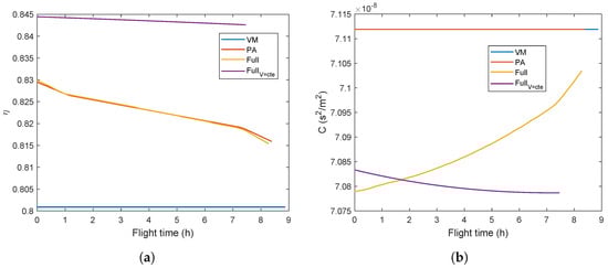
Figure 5.
Evolution of (a) the propeller efficiency and (b) the specific fuel consumption C during the cruise for the Von Mises (blue), PA (red), and full (yellow) models, and the constant speed program FullV=cte (magenta). Since the time of flight (abscissas of the plots) is different for each case, the ending points of each curve are also different.
Therefore, the similarity in and C makes the associated propulsion systems of the PA and full models practically interchangeable, which explains their identical behavior during optimal flight (Table 2). Hence, for the full model, it was also found that the required and available powers were almost the same, and C was approximately constant.
5.3.3. Characteristics of Optimal Flights
Some of the previous results can be analyzed in more detail from the evolution of different features through the optimal cruise flight. Hence, in Figure 6 we present the time variation of the state variables and the control for all the models and programs appearing in Table 2.
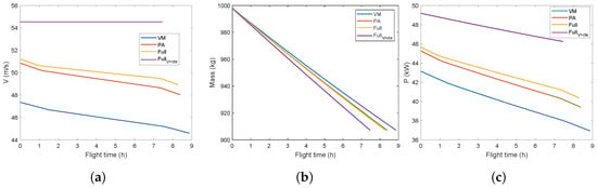
Figure 6.
Evolution of the state variables (a) V, (b) m, and (c) P through the cruise. The cases considered, the color codes, and the observations are the same as those described in the caption of Figure 5.
The variations of the state variables and the control are moderate during the flight, about or below. This is a consequence of the corresponding low value of the cruise fuel-weight fraction of our Piper Cherokee PA-28 (Table 1), as can be also seen in the evolution of m (Figure 6b).
This is particularly the case of the velocity for the three functional models of the propulsive system. Their variations are below 6%, which entails that the respective optimal flights, giving the maximum cruise range, could be substituted by constant speed programs associated to each scenario. Such approach would hardly penalize the maximum distance flown, a common feature for this kind of propeller-driven light aircraft, as discussed when and C are constant in Hale ([2], chapter 6).
As can be observed in Figure 6, the evolution of the state variables and the control shows similar trends for all models. For m, they can be accurately described by straight lines with negative slopes. In the case of V and P, such a description does not fit so well due to the slight bending of the curves at the beginning and the end of the flight. This is related to the lack of boundary conditions for the velocity in the optimal control problem, as it was previously pointed out.
The decrease in velocity with time for the optimal cases is related to flying at an approximately constant angle of attack in the level cruise, where the lift equals the weight. As in the case of the Von Mises model, such a circumstance along with the burning of fuel, i.e., the decrease in mass, implies a reduction in the value of velocity, as well as in power and required power.
This fact is clearly shown in Figure 7a, where we have displayed the evolution of the aerodynamic efficiency. It can be seen that the optimal flights for the different models of the propulsive system are performed with an almost constant aerodynamic efficiency, with its particular value arising from the condition of maximizing the range.
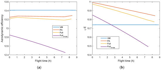
Figure 7.
Evolution of (a) the aerodynamic efficiency E and (b) during the cruise. The considered cases, color codes, and observations are the same as those described in the caption of Figure 5.
Indeed, for the Von Mises model, that condition is fulfilled exactly. In the case of the PA and full models, the aerodynamic efficiency is also practically constant, with variations that do not exceed 0.5%. So, the optimal flights also keep an almost fixed value of the aerodynamic efficiency for the more complex propulsive system models.
However, in contrast to the Von Mises situation, the value of the aerodynamic efficiency is not the maximum , although it is not far from it. This fact is common to the PA and full models, but it is easier understood in terms of the PA model that already incorporates a V dependence in .
Expressing the functional (Equation (16)) in terms of and E, and using m as the independent variable, introducing the available and required powers (Equation (17)), the range is maximum when maximizing
In the classical Breguet equation , and are constant, so Equation (23) is recovered (Anderson [3], chapter 5). For the PA model, C is constant. Moreover, during the cruise we obtain that the required power is approximately equal to the available power, . So, we can write
The former integral takes its largest value when the product is at its maximum for each particular m. That mass carries with it a value of the velocity V, so and E can be viewed alternatively as functions of V instead of m. Thus, one would look for the value of V maximizing , which, in turn, could be used to define the singular arc.
The velocity V that provodes the largest value of E, i.e., the one of the Von Mises model, corresponds to that with the minimum drag force in the cruise flight (e.g., Anderson [3], chapter 5). Such velocity is a bit low, which entails a small value of (Equation (27)). Hence, the resulting velocity that maximizes for the PA and the Full models is larger than the Von Mises speed, as shown in Figure 6. In contrast, the velocity that provides the maximum value of is high and implies that the aerodynamic efficiency is small, as derived, for example, from the case of the the constant speed program in Figure 7a.
Therefore, the instantaneous value of the velocity maximizing results from a balance between obtaining the maximum E and the maximum , compatible with the other conditions of the optimal problem. This explains why in the optimal flight E and are lower than the respective maximum values.
In addition, the maximum slightly decreases as the mass is burnt when depends on V. This can be viewed in Figure 7b. In the PA model, the value of V, for each m, which maximizes , can be computed numerically from Equations (2) and (27) with . Except for very tiny differences due to the assumed approximations, it leads to the same plot as in Figure 7b, obtained with the numerical transcription method with regularization. For the Von Mises model, the maximum of is constant for all the values of m, , since, in this case, does not vary. For the other cases, such a reduction in the maximum value of together with the small absolute variation of leads to an almost constant value for the aerodynamic efficiency, i.e., of the angle of attack.
In view of their similarity, previous discussion about maximizing to get the maximum cruise range explained for the PA model, as it provides an easier physical visualization, can be extended to the full model.
The proposed methodology offers a valuable solution to compute optimal flights of light aircraft or unmanned aerial vehicles. This can be applied to optimize the design requirements and meet the specifications for these types of aerospace vehicles according to their planned missions.
6. Conclusions
The problem of maximizing the range of a propeller-driven aircraft in a level flight cruise has been solved, i.e., the way in which the aircraft must be controlled to obtain the largest range from a given amount of fuel. It has been tackled from the point of view of optimal control. As representative of light aircraft, we selected a notional Piper Cherokee PA-28.
Our model of the propulsive system is realistic and goes further than just taking a constant specific fuel consumption and propeller efficiency, as in previous studies (e.g., Cavcar and Cavcar [23]). For the engine, we considered potential dependencies of the power P on velocity through the maximum power delivered by the engine and of the fuel flow rate on velocity and power. For the propeller, the propulsive efficiency is assumed to be a function of the velocity and the power. The particular functional forms are derived from models based on polynomial expressions fitted in a least-square sense to the data.
The former model, referred to as the full model, is cumbersome. Hence, we also built two simplified models. The first one is the Von Mises model, the common case studied in the literature, characterized by a constant C and obtained from some representative values of P and V for the mission. The second characterization, named the PA model, keeps C constant, as in the Von Mises model, but assumes that is a function of the velocity.
We obtained the corresponding maximum range for the three models by means of a numerical algorithm that combines a transcription method with a regularization term. The inclusion of the regularization term is necessary because the Von Mises and the PA models lead to singular optimal problems. In this way, we get an automated numerical method to solve optimal problems in flight mechanics, regardless of whether they are singular or not, providing a useful procedure to determine the performance of propeller-driven aircrafts.
The performance of the numerical method was validated against the analytical solution of the Breguet equations, obtaining that the differences for the maximum range, the state variables, and the control were below 0.6% of relative error.
The results for the full model provided a maximum range that reached 1491.52 km with a time of flight of 8.28 h. We also computed the solution for a non-optimal flight constructed from the full model, but flown with a characteristic constant speed. In this case, the range was reduced by about 2.0%, but there was a significant saving of the time of flight, about 49 min. Hence, this constant speed program is very convenient for this kind of aircraft if there are no stringent conditions in the maximum range to be achieved.
This represents an important distinction with respect to the turbojet case (Pargett and Ardema [17]), where the difference in the constant speed flight was about 10%. The main reason is that, for propeller-driven light aircraft, the value of the cruise fuel-weight fraction is relatively low, , compared to the turbojet situation, .
However, the evolution of the state variables, the control, and some flight quantities during the constant speed flight, are quite different from the optimal flight of the full model.
The Von Mises model presented small relative errors, although they were quite a bit larger for the time of flight than for the range. For its part, the flight features of the PA model stay very close to the full model ones. This shows that the approximation employed to constructed the PA model in the cruise flight is quite accurate. In turn, as for this model the propeller efficiency is a function of V, it is easier to get insight into the physics of the optimal flight. This information can be of help to select the performance parameters of the propeller-driven light aircraft.
Specifically, in contrast to the classical Breguet case (Von Mises model), the flight was performed with almost constant aerodynamic efficiency E, but not maximum. The reason was that, as , the optimal flight was achieved by maximizing with respect the velocity, not just E. This led to almost constant values of and E, but not maximum ones. Since the dependence of C on P for the full model was quite flat, such behavior was also reproduced for this case.
Finally, we present a summarizing table (Table 3) to outline the main findings and conclusions of the study that has been conducted, highlighting the more interesting aspects of the models that have been considered.
Table 3.
Summary of the findings and conclusions of the analysis for the optimal cruise range, including the characteristics of the different models.
It can be seen how the full model provides the best results in terms of accuracy as it is the most realistic representation of the aircraft features. In this way, it can be employed for the precise characterization of the mission. It requires deriving a functional model for the propulsive system, e.g., specific fuel consumption and propeller efficiency, of the aircraft, for which it is necessary to have enough available data coming from experimental testing or simulations of the engine and the propeller.
For its part, the PA model showed very similar solutions, almost reproducing the results of the full model. Therefore, it constitutes a very good approximation of the actual behavior with computational times equivalent to those of the full model. In return, it provides a good and intuitive physical insight into the solution. This is due to the fact that, starting from the engine and propeller characterization of the full model, some dependencies in the specific fuel consumption and the propeller efficiency with respect to the power and velocity are skipped. As a result, the relation between the state variables and the propulsive system of the optimal flight is grasped more easily.
As it was highlighted before, both the Von Mises model and the Breguet formulation seem to be a good compromise between simplicity and moderate accuracy, which explains why this solution is highly valued in the conceptual design of an airplane. It must be noted that despite in both Von Mises and Breguet models the propulsive system model is simpler, the selection of the respective constants is of great relevance. Here, differences of only around 10% are obtained as such values are derived from the full model. However, if they are not taken carefully in order to be representative of the actual behavior of the aircraft, the variations can be significantly increased.
In the case of the FullV=cte model, it provides a solution corresponding to a different program, which does not optimize the range but reduces the time of flight. These results can be relevant from the perspective of propeller-driven light aircraft, where reducing the time of flight becomes more important than getting the maximum range.
Our approach admits natural extensions in several directions. For example, the entire flight profile could be considered, which would augment the size of the problem, or additional restrictions that might incorporate some constrains due to traffic control limitations could be introduced. Moreover, other performance indexes different from the range might be studied (e.g., Boucher et al. [50]), such as the endurance, the direct operating costs, etc.
It is also possible to increment the number of controls, incorporating the fuel mixture and the revolutions of the engine in the functional model of the propulsive system. This would require us to have a detailed characterization of both the engine and the propeller for different flight regimes.
The method is also suitable to be applied to other aircraft with a reciprocating engine and a propeller, like unmanned aerial vehicles (UAV), and, with the corresponding modifications, to different propulsive systems or, even, aerospace platforms. The combination of a transcription method with a regularization term allows the numerical resolution of that kind of problem. Such solutions are quick and reasonably accurate; hence, they are of interest in the design phases of aerospace vehicles.
Author Contributions
Conceptualization, A.D., D.D. and A.E.; methodology, A.D. and A.E.; software, A.D.; validation, A.D. and A.E.; formal analysis, A.D., C.R., D.D. and A.E.; investigation, A.D. and A.E.; resources, A.D., C.R., D.D. and A.E.; data curation, A.D., C.R., D.D. and A.E.; writing—original draft preparation, A.D. and A.E.; writing—review and editing, A.D., C.R., D.D. and A.E.; visualization, A.D., C.R., D.D. and A.E.; supervision, D.D. and A.E.; project administration, A.D., C.R., D.D. and A.E. All authors have read and agreed to the published version of the manuscript.
Funding
This research received no external funding.
Data Availability Statement
The original contributions presented in the study are included in the article, and further inquiries can be directed to the corresponding author/s.
Conflicts of Interest
The authors declare no conflicts of interest.
Abbreviations
The following abbreviations are used in this manuscript:
| V | velocity |
| m | mass |
| available power | |
| required power | |
| T | thrust |
| D | drag force |
| L | lift force |
| fuel flow rate | |
| g | gravitational acceleration |
| ISA | International Standard Atmosphere |
| air density | |
| S | reference area of the airplane |
| zero-lift drag coefficient | |
| K | induced drag coefficient |
| range | |
| initial time | |
| final time | |
| initial mass | |
| final mass | |
| mass of fuel | |
| mass of the aircraft fully equipped plus the payload (and the reserve fuel) | |
| propulsive efficiency | |
| P | shaft brake power |
| rotational speed of the propeller | |
| diameter of the propeller | |
| dimensionless thrust coefficient | |
| dimensionless power coefficient | |
| rpm | revolutions per minute |
| blade angle | |
| blade angle at 75% of the radial distance | |
| J | advance ratio |
| the throttle power parameter | |
| n | rotational speed of the engine |
| C | specific fuel consumption |
| maximum aerodynamic efficiency | |
| reference velocity | |
| reference available power | |
| reference thrust | |
| VM | Von Mises |
| PA | Parget and Ardema |
| N | number of subintervals |
| defects | |
| regularization term | |
| UAV | unmanned air vehicles |
References
- Miele, A. Flight Mechanics. Volume 1: Theory of Flight Paths; Addison-Wesley: Boston, MA, USA, 1962. [Google Scholar]
- Hale, F.J. Introduction to Aircraft Performance, Selection, and Design; Wiley: New York, NY, USA, 1984. [Google Scholar]
- Anderson, J.D. Aircraft Performance and Design; WCB/McGraw-Hill: Boston, MA, USA, 1999; Volume 1. [Google Scholar]
- Bryson, A.E. Optimal control-1950 to 1985. IEEE Control Syst. Mag. 1996, 16, 26–33. [Google Scholar] [CrossRef]
- Saucier, A.; Maazoun, W.; Soumis, F. Optimal speed-profile determination for aircraft trajectories. Aerosp. Sci. Technol. 2017, 67, 327–342. [Google Scholar] [CrossRef]
- Hargraves, C.; Paris, S. Direct trajectory optimization using nonlinear programming and collocation. J. Guid. Control Dyn. 1987, 10, 338–342. [Google Scholar] [CrossRef]
- Morante, D.; Sanjurjo Rivo, M.; Soler, M. A Survey on Low-Thrust Trajectory Optimization Approaches. Aerospace 2021, 8, 88. [Google Scholar] [CrossRef]
- Betts, J.T. Survey of numerical methods for trajectory optimization. J. Guid. Control Dyn. 1998, 21, 193–207. [Google Scholar] [CrossRef]
- Rao, A.V. A survey of numerical methods for optimal control. Adv. Astronaut. Sci. 2009, 135, 497–528. [Google Scholar]
- Conway, B.A. A survey of methods available for the numerical optimization of continuous dynamic systems. J. Optim. Theory Appl. 2012, 152, 271–306. [Google Scholar] [CrossRef]
- Mai, T.; Mortari, D. Theory of functional connections applied to quadratic and nonlinear programming under equality constraints. J. Comput. Appl. Math. 2022, 406, 113912. [Google Scholar] [CrossRef]
- Leake, C.; Johnson, H.; Mortari, D. The Theory of Functional Connections: A Functional Interpolation Framework with Applications; Lulu Press, Inc.: Morrisville, NC, USA, 2022. [Google Scholar]
- Betts, J.T.; Cramer, E.J. Application of Direct Transcription to Commercial Aircraft Trajectory Optimization. J. Guid. Control Dyn. 1995, 18, 151–159. [Google Scholar] [CrossRef]
- González-Arribas, D.; Soler, M.; Sanjurjo-Rivo, M.; Kamgarpour, M.; Simarro, J. Robust aircraft trajectory planning under uncertain convective environments with optimal control and rapidly developing thunderstorms. Aerosp. Sci. Technol. 2019, 89, 445–459. [Google Scholar] [CrossRef]
- Menon, P.K.A. Study of aircraft cruise. J. Guid. Control Dyn. 1989, 12, 631–639. [Google Scholar] [CrossRef]
- Bell, D.J.; Jacobson, D.H. Singular Optimal Control Problems; Elsevier: Amsterdam, The Netherlands, 1975. [Google Scholar]
- Pargett, D.M.; Ardema, M.D. Flight Path Optimization at Constant Altitude. J. Guid. Control Dyn. 2007, 30, 1197–1201. [Google Scholar] [CrossRef]
- Kelley, H.; Kopp, R.; Moyer, H.G. 3 singular extremals. In Mathematics in Science and Engineering; Elsevier: Amsterdam, The Netherlands, 1967; Volume 31, pp. 63–101. [Google Scholar] [CrossRef]
- Rivas, D.; Valenzuela, A. Compressibility Effects on Maximum Range Cruise at Constant Altitude. J. Guid. Control Dyn. 2009, 32, 1654–1658. [Google Scholar] [CrossRef]
- Franco, A.; Rivas, D. Minimum-Cost Cruise at Constant Altitude of Commercial Aircraft Including Wind Effects. J. Guid. Control Dyn. 2011, 34, 1253–1260. [Google Scholar] [CrossRef]
- Ardema, M.D.; Asuncion, B.C. Flight path optimization at constant altitude. In Variational Analysis and Aerospace Engineering; Springer: New York, NY, USA, 2009; pp. 21–32. [Google Scholar] [CrossRef]
- Von Mises, R. Theory of Flight; McGraw-Hill: New York, NY, USA, 1945. [Google Scholar]
- Cavcar, M.; Cavcar, A. Optimum Range and Endurance of a Piston Propeller Aircraft with Cambered Wing. J. Aircr. 2005, 42, 212–217. [Google Scholar] [CrossRef]
- Lowry, J. Performance of Light Aircraft; AIAA Education Series; American Institute of Aeronautics and Astronautics: Reston, VA, USA, 1999. [Google Scholar]
- Tulapurkara, E.; Ananth, S.; Kulkarni, T.M. Performance Analysis of a Piston Engined Airplane-Piper Cherokee PA-28-180; Technical Report REPORT NO: AE TR 2007-1; Department of Aerospace Engineering, IIT Madras: Chennai, India, 2007. [Google Scholar]
- Donateo, T.; Totaro, R. Hybridization of training aircraft with real world flight profiles. Aircr. Eng. Aerosp. Technol. 2019, 91, 353–365. [Google Scholar] [CrossRef]
- Rostami, M.; Chung, J.; Neufeld, D. Vertical tail sizing of propeller-driven aircraft considering the asymmetric blade effect. Proc. Inst. Mech. Eng. Part G J. Aerosp. Eng. SAGE Publ. 2021, 236, 1184–1195. [Google Scholar] [CrossRef]
- Bergmann, D.; Denzel, J.; Pfeifle, O.; Notter, S.; Fichter, W.; Strohmayer, A. In-flight Lift and Drag Estimation of an Unmanned Propeller-Driven Aircraft. Proc. Inst. Mech. Eng. Part G J. Aerosp. Eng. SAGE Publ. 2021, 8, 43. [Google Scholar] [CrossRef]
- Bravo, G.; Praliyev, N.; Veress, Á. Performance analysis of hybrid electric and distributed propulsion system applied on a light aircraft. Energy 2021, 6, 1184–1195. [Google Scholar] [CrossRef]
- Betts, J.T. Practical Methods for Optimal Control and Estimation Using Nonlinear Programming; SIAM: Philadelphia, PA, USA, 2010. [Google Scholar]
- Zheng, X.; Xia, F.; Lin, D.; Jin, T.; Su, W.; He, S. Constrained Parameterized Differential Dynamic Programming for Waypoint-Trajectory Optimization. Aerospace 2024, 11, 420. [Google Scholar] [CrossRef]
- Li, R.; Yang, Z.; Yan, G.; Jian, L.; Li, G.; Li, Z. Robust Approximate Optimal Trajectory Tracking Control for Quadrotors. Aerospace 2024, 11, 149. [Google Scholar] [CrossRef]
- Ruijgrok, G. Elements of Airplane Performance; VSSD Pub: Delft, The Netherlands, 2009. [Google Scholar]
- Torenbeek, E. Synthesis of Subsonic Airplane Design; Springer: New York, NY, USA, 1982. [Google Scholar]
- Lycoming. Operator’s Manual: O-360, HO-360, IO-360, AIO-360, HIO-360 & TIO-360 Series; Technical Report; Lycoming: Williamsport, PA, USA, 2005. [Google Scholar]
- Piper Aircraft. A Brief History of Piper Aircraft; Piper Aircraft. 2022. Available online: https://www.piper.com/blog/piper-history/ (accessed on 18 September 2024).
- Corporation, P.A. Cherokee 180, PA-28-180. In Owner’s Handbook (761-513); Technical Report; Piper Aircraft Corporation: Vero Beach, FL, USA, 1973. [Google Scholar]
- Federal Aviation Administration. Type Certyficate Data Sheet No. 2A13; Technical Report; U.S. Department of Transportation: Washington, DC, USA, 2009.
- McCormick, B.W. Aerodynamics, Aeronautics, and Flight Mechanics; John Wiley and Sons: Hoboken, NJ, USA, 1995. [Google Scholar]
- Abbott, I.H.; Von Doenhoff, A.E.; Stivers, L., Jr. Summary of Airfoil Data; Technical Report NACA Report 824; NASA Technical Reports Server; The National Aeronautics and Space Administration (NASA): Washington, DC, USA, 1945.
- Cavcar, M. Bréguet Range Equation? J. Aircr. 2006, 43, 1542–1544. [Google Scholar] [CrossRef]
- Schwartz, A.L. Theory and Implementation of Numerical Methods Based on Runge-Kutta Integration for Solving Optimal Control Problems; University of California: Berkeley, CA, USA, 1996. [Google Scholar]
- Jacobson, D.; Gershwin, S.; Lele, M. Computation of optimal singular controls. IEEE Trans. Autom. Control 1970, 15, 67–73. [Google Scholar] [CrossRef]
- Pager, E.R.; Rao, A.V. Method for solving bang-bang and singular optimal control problems using adaptive Radau collocation. Comput. Optim. Appl. 2022, 81, 857–887. [Google Scholar] [CrossRef]
- Dadebo, S.; McAuley, K.; McLellan, P. On the computation of optimal singular and bang–bang controls. Optim. Control Appl. Methods 1998, 19, 287–297. [Google Scholar] [CrossRef]
- Gill, P.E.; Murray, W.; Saunders, M.A.; Wong, E. User’s guide for SQOPT Version 7.7: Software for large-scale linear and quadratic programming. In Center for Computational Mathematics Report CCoM 19-01; University of California: San Diego, CA, USA, 2019. [Google Scholar]
- Silva, C.; Trelat, E. Smooth Regularization of Bang-Bang Optimal Control Problems. IEEE Trans. Autom. Control 2010, 55, 2488–2499. [Google Scholar] [CrossRef]
- Zelikin, M.I.; Borisov, V. Theory of Chattering Control; Birkhäuser: Boston, MA, USA, 1994. [Google Scholar] [CrossRef]
- Lavezzi, G.; Guye, K.; Cichella, V.; Ciarcià, M. Comparative Analysis of Nonlinear Programming Solvers: Performance Evaluation, Benchmarking, and Multi-UAV Optimal Path Planning. Drones 2023, 7, 487. [Google Scholar] [CrossRef]
- Boucher, O.; Bellouin, N.; Clark, H.; Gryspeerdt, E.; Karadayi, J. Comparison of Actual and Time-Optimized Flight Trajectories in the Context of the In-Service Aircraft for a Global Observing System (IAGOS) Programme. Aerospace 2023, 10, 744. [Google Scholar] [CrossRef]


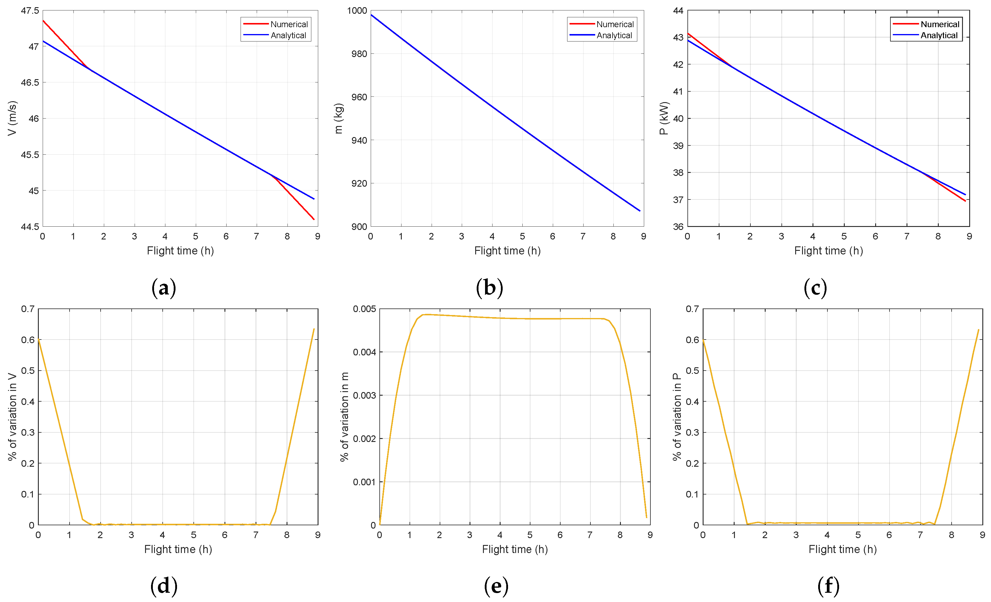
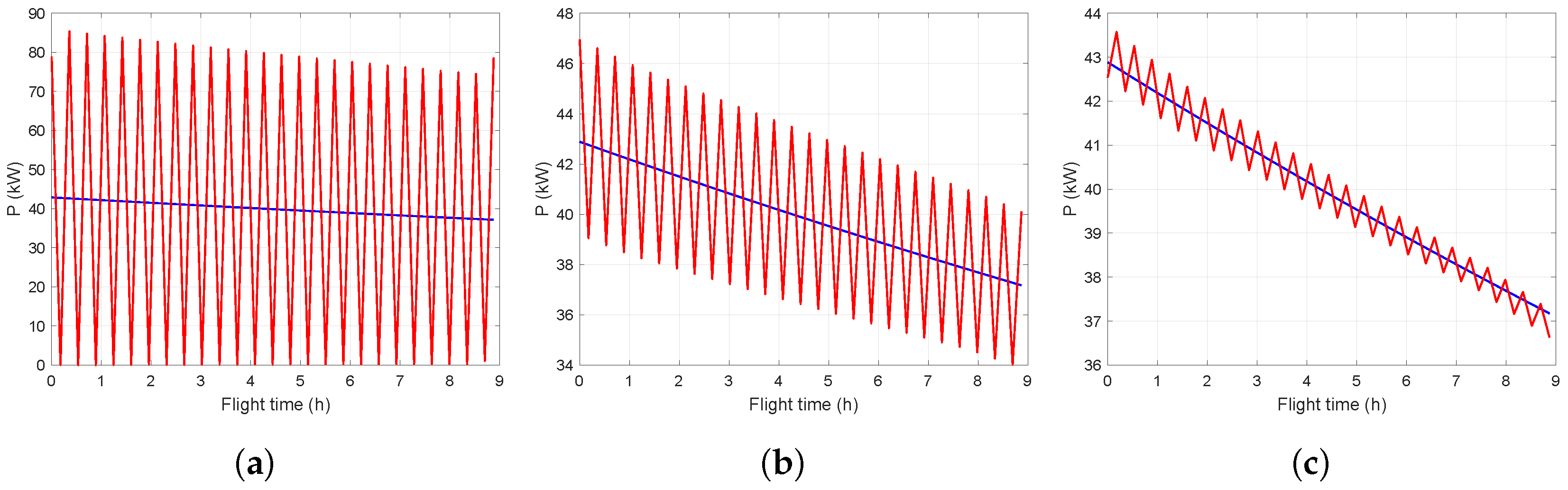
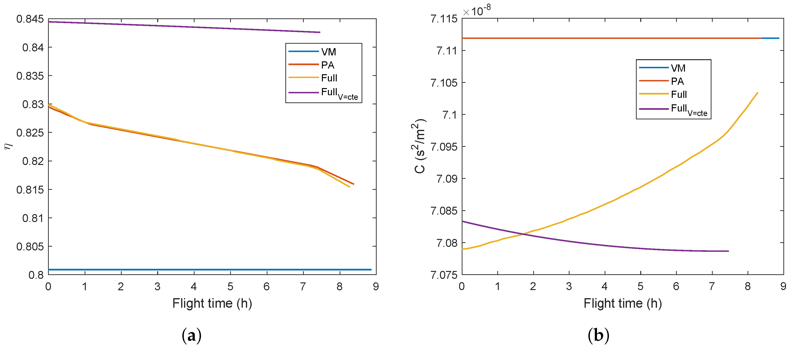
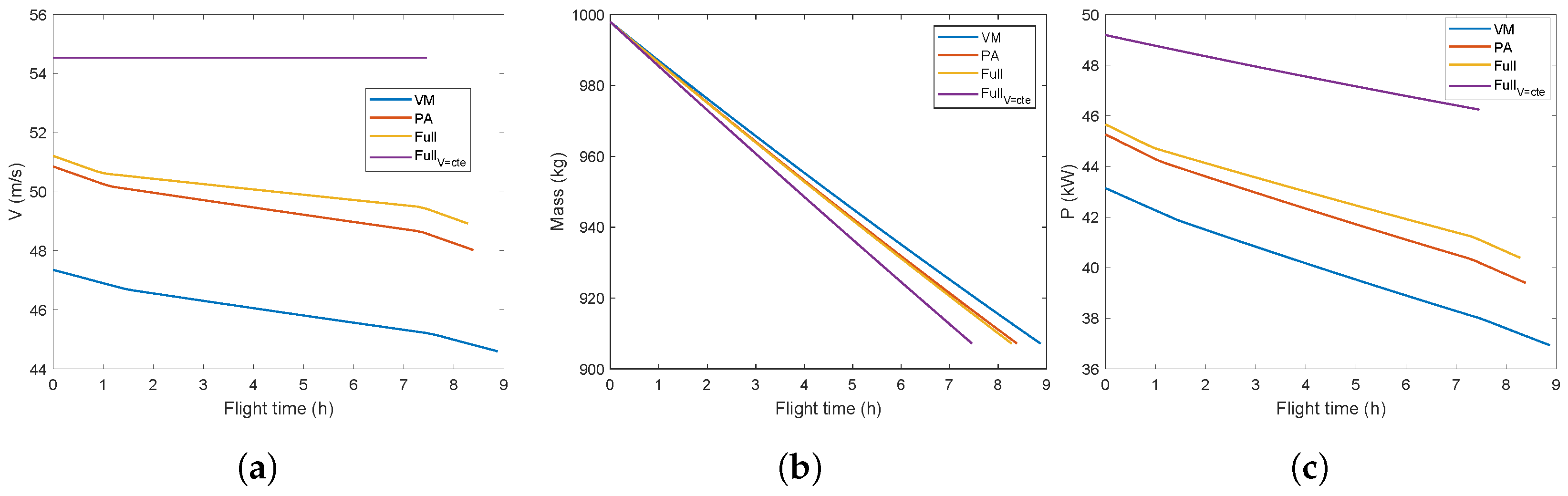

Disclaimer/Publisher’s Note: The statements, opinions and data contained in all publications are solely those of the individual author(s) and contributor(s) and not of MDPI and/or the editor(s). MDPI and/or the editor(s) disclaim responsibility for any injury to people or property resulting from any ideas, methods, instructions or products referred to in the content. |
© 2024 by the authors. Licensee MDPI, Basel, Switzerland. This article is an open access article distributed under the terms and conditions of the Creative Commons Attribution (CC BY) license (https://creativecommons.org/licenses/by/4.0/).