Abstract
The geometric correction of thermal infrared (TIR) orthophotos generated by unmanned aerial vehicles (UAVs) presents significant challenges due to low resolution and the difficulty of identifying ground control points (GCPs). This study addresses the limitations of real-time kinematic (RTK) UAV data acquisition, such as network instability and the inability to detect GCPs in TIR images, by proposing a method that utilizes RGB orthophotos as a reference for geometric correction. The accelerated-KAZE (AKAZE) method was applied to extract feature points between RGB and TIR orthophotos, integrating binary descriptors and absolute coordinate-based matching techniques. Geometric correction results demonstrated a significant improvement in regions with stable and changing environmental conditions. Invariant regions exhibited an accuracy of 0.7~2 px (0.01~0.04), while areas with temporal and spatial changes saw corrections within 5~7 px (0.10~0.14 m). This method reduces reliance on GCP measurements and provides an effective supplementary technique for cases where GCP detection is limited or unavailable. Additionally, this approach enhances time and economic efficiency, offering a reliable alternative for precise orthophoto generation across various sensor data.
1. Introduction
The rapid development of unmanned aerial vehicle (UAV) technology has enabled the generation of high-resolution orthophotos for various applications, including geomatics and remote sensing [1,2]. UAV-based photogrammetry offers significant advantages over traditional methods, particularly in areas that are difficult to access or that cover large geographical regions [3,4]. Conventional aerial or satellite-based image acquisition methods, while useful for wide-area mapping, have limitations in terms of cost, time, and resolution [5,6,7]. In contrast, UAVs can be deployed quickly and repeatedly to capture high-quality images, making them an ideal tool for generating orthophotos in diverse environmental conditions [8].
However, a major challenge in UAV-based photogrammetry, especially when using thermal infrared (TIR) sensors, is achieving accurate geometric correction [9]. Unlike RGB imagery, where ground control points (GCPs) can be easily identified, TIR images suffer from low resolution and difficulty in detecting GCPs due to the nature of thermal data [10,11]. This often results in geometric distortions that reduce the accuracy of the orthophotos. Although real-time kinematic (RTK) UAVs have been employed to improve positional accuracy, they can be unreliable in environments with network instability, making it challenging to acquire precise location data [12,13,14].
Previous studies have primarily focused on correcting geometric distortions in RGB orthophotos using relative and absolute coordinate methods [15,16]. However, there is limited research on geometric correction between multi-sensor orthophotos, particularly between TIR and RGB images. TIR images present unique challenges due to their low resolution and sensitivity to environmental factors such as time and temperature variations, which complicate feature matching and geometric correction.
Thus, this study aims to address these challenges by exploring a novel approach that uses RGB orthophotos as reference images for the geometric correction of TIR orthophotos. The method focuses on extracting and matching feature points between the two image types using the accelerated-KAZE (AKAZE) method, integrating binary descriptors and absolute coordinate-based matching techniques to achieve high accuracy in geometric correction, even in regions with significant temporal and spatial changes.
2. Materials
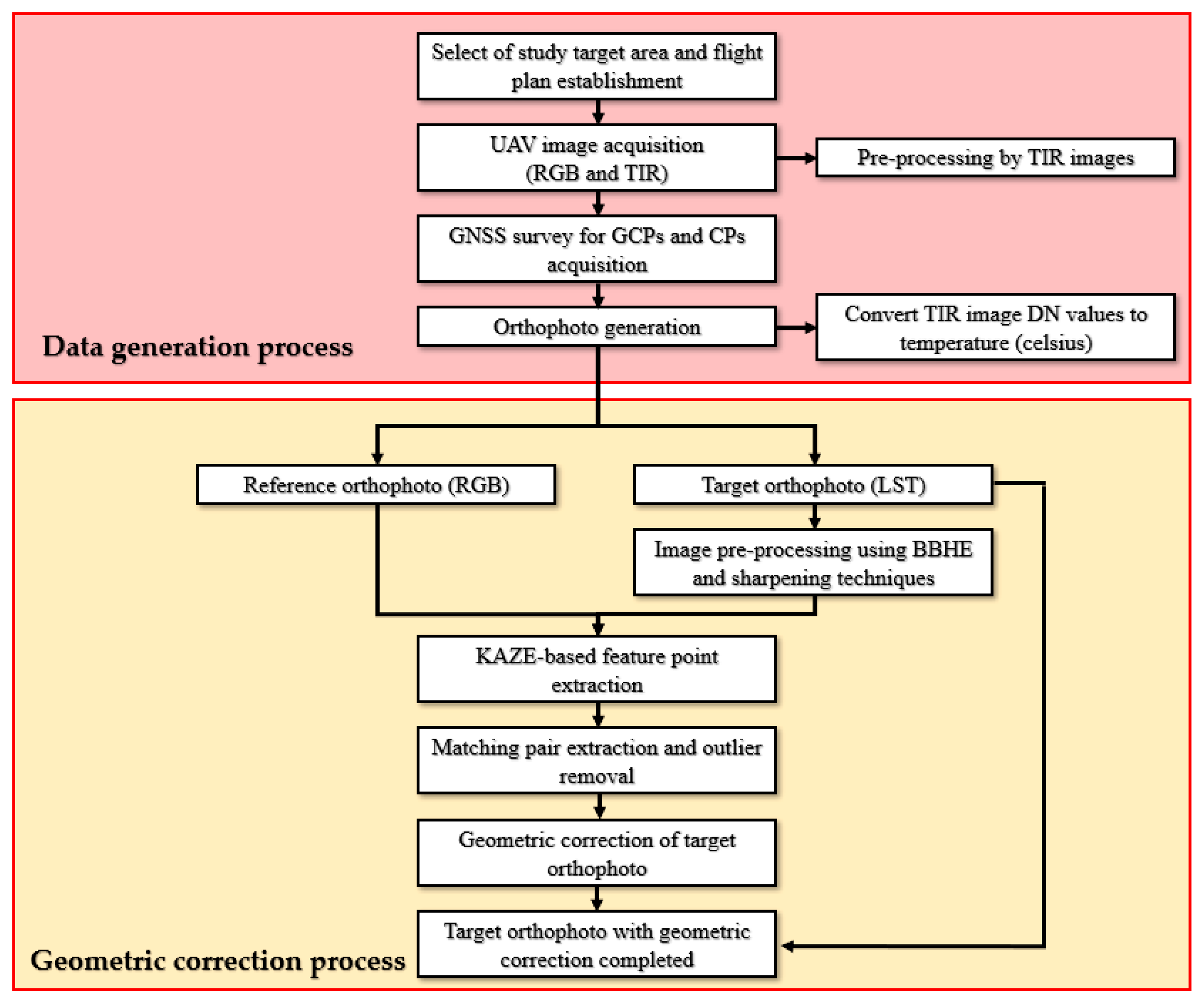
Figure 1 shows the overall research flow chart, which outlines the main steps followed in this study. Each step in the flow chart represents a critical phase of the research, ensuring the accurate geometric correction of TIR orthophotos using RGB reference images.
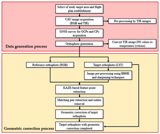
Figure 1.
Illustrates the flow chart of the entire process, from data collection to result evaluation.
2.1. Study Area and Equipment
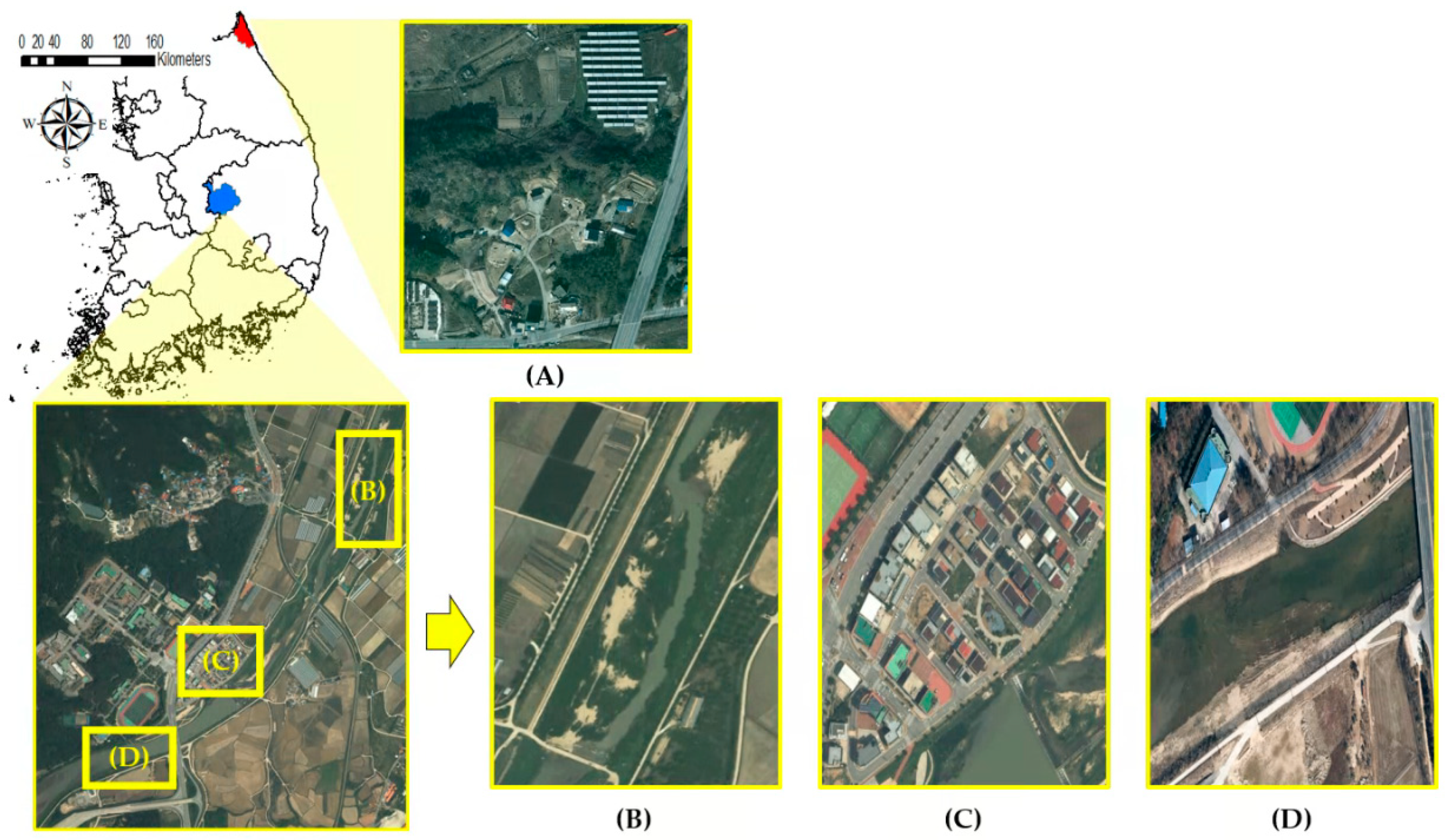
Four research sites were selected for investigation in this work. Study area A is located in Yongchon-ri, Toseong-myeon, Goseong-gun, Gangwon-do in South Korea (latitude: 38.234; longitude: 128.570). In 2019, a forest fire in Gangwon-do damaged the mountain area and some parts of a village. Many restorations on these damaged portions were performed in 2023. Study site A currently has various land covers, including buildings, mountains, fields, and roads. Study sites B (latitude: 36.375; longitude: 128.147), C (latitude: 36.377; longitude: 128.149), and D (latitude: 36.383; longitude: 128.155) are located in Gajang-dong, Sangju-si, Gyeongsangbuk-do in South Korea. Sites B and D are small streams in the city center, with the amount of water in area D being higher than that in area B. This area was selected to study the possibility of a geometric correction of the river and surrounding areas. The land covers of these two regions differed from each other, which was why each was selected. Study area C is a residential area in front of the Sangju campus of the Kyungpook National University in South Korea. It was selected for geometric correction on areas concentrated with buildings. All the remaining study sites, except for C, are areas that have changed over time since 2019 and 2020. Therefore, only four study sites were selected to confirm the non-changing and changing areas (Figure 2).
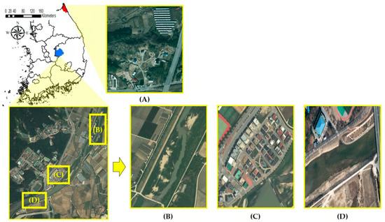
Figure 2.
Study areas: (A) latitude: 38.234 and longitude: 128.570; (B) latitude: 36.375 and longitude: 128.147; (C) latitude: 36.377 and longitude: 128.149; and (D) latitude: 36.383 and longitude: 128.155.
Three rotary-wing UAVs (DJI, Shenzhen, China) were used in this study. One UAV was used to produce RGB-based orthophotos, while the other two were used to acquire TIR images from sensors with different specifications. To evaluate the results of geometric correction based on the type of TIR sensor, images were acquired using two different TIR sensors. An Inspire 2 UAV was used to capture RGB images. It weighed 3440 g and had a maximum liftoff altitude of 2500 m above the ground, a maximum wind speed resistance of 10 m/s, and a maximum flight time of 27 min. An Inspire 1 UAV was used to acquire the TIR images. It weighed 2935 g and had a maximum speed of 22 m/s, a maximum flight altitude of 4500 m above ground level, and a maximum wind resistance of 10 m/s. A full-capacity battery allows approximately 18 min of flying. The UAVs acquire RGB and TIR images using Matrice 300 RTK. In this study, however, it was used to acquire the TIR images. The Matrice 300 RTK weighed 3600 g and had a maximum speed of 23 m/s, a maximum flight altitude of 6000 m, a maximum wind speed resistance of 15 m/s, and a maximum flight time of 55 min. The RTK signal was disconnected, and data acquisition was performed.
The three sensors used in this work were from DJI. The Zenmuse XT TIR sensor was manufactured by FLIR (Wilsonville, OR, USA), while the other sensors (Zenmuse X4S and Zenmuse H20T) were manufactured by DJI. The first sensor was the Zenmuse X4S RGB sensor, which was compatible with Inspire 2. It weighed 270 g and had a resolution of 5472 × 3648, a field of view (FOV) of 84°, and a focal length of 8.8 mm. The second sensor was the Zenmuse XT TIR sensor, which was exclusive to Inspire 1 and manufactured by FLIR, as well. It weighed 253 g and had a resolution of 640 × 512, an FOV of 45° × 37°, and a focal length of 13 mm. The third and last sensor was the Zenmuse H20T, a dual sensor with RGB and TIR sensors. It was a Matrice 300 RTK-only sensor that weighed 828 g and had an RGB resolution of 4056 × 3040, a TIR of 640 × 512, a FOV of 82.9°, a TIR of 40.6°, and a focal length of RGB 4.5 mm and TIR 13.5 mm. Only the TIR sensor was used herein.
Trimble R8s, which have 440 channels, were used for the GCP and CP survey. The satellites in Trimble R8s can freely be combined as the number of channels increases, thereby enabling high-accuracy positioning. The satellite signals can receive the global positioning system (GPS), GLONASS, SBAS, Galileo, and BeiDou. In this study, surveys of GCPs and CPs are acquired through VRS survey, one of the network-RTK methods. In this study, GPS signals were sufficient to obtain ground coordinates during VRS surveying, so the signals L1C/A, L1C, L2C, L2E, and L5 were received and used for the measurements and CPs. In this study, surveys of GCPs and CPs are acquired through VRS survey, one of the network-RTK methods. The VRS surveying accuracy of Trimble R8s is specified as follows: 8 mm + 0.5 ppm root mean square error (RMSE) horizontally and 15 mm + 0.5 ppm RMSE vertically.
2.2. Data Acquisition
2.2.1. UAV Data Acquisition
The flight planning application differed for each type of UAV and sensor; therefore, two types of flight planning applications were used in this study. The flight planning software can set the shooting environment (e.g., flight plan and height, speed, and overlap). Information, such as the capture interval, battery status, reception status, and real-time video, can be checked depending on the shooting range, speed, and overlap. Inspire 1 and 2, Pix4d Capture, and Matrice 300 RTK used DJI Pilot. Table 1 presents the UAV image acquisition dates. All images were acquired between 12:00 and 13:00 when the sun was at its highest.

Table 1.
Orthophoto acquisition date information by research field.
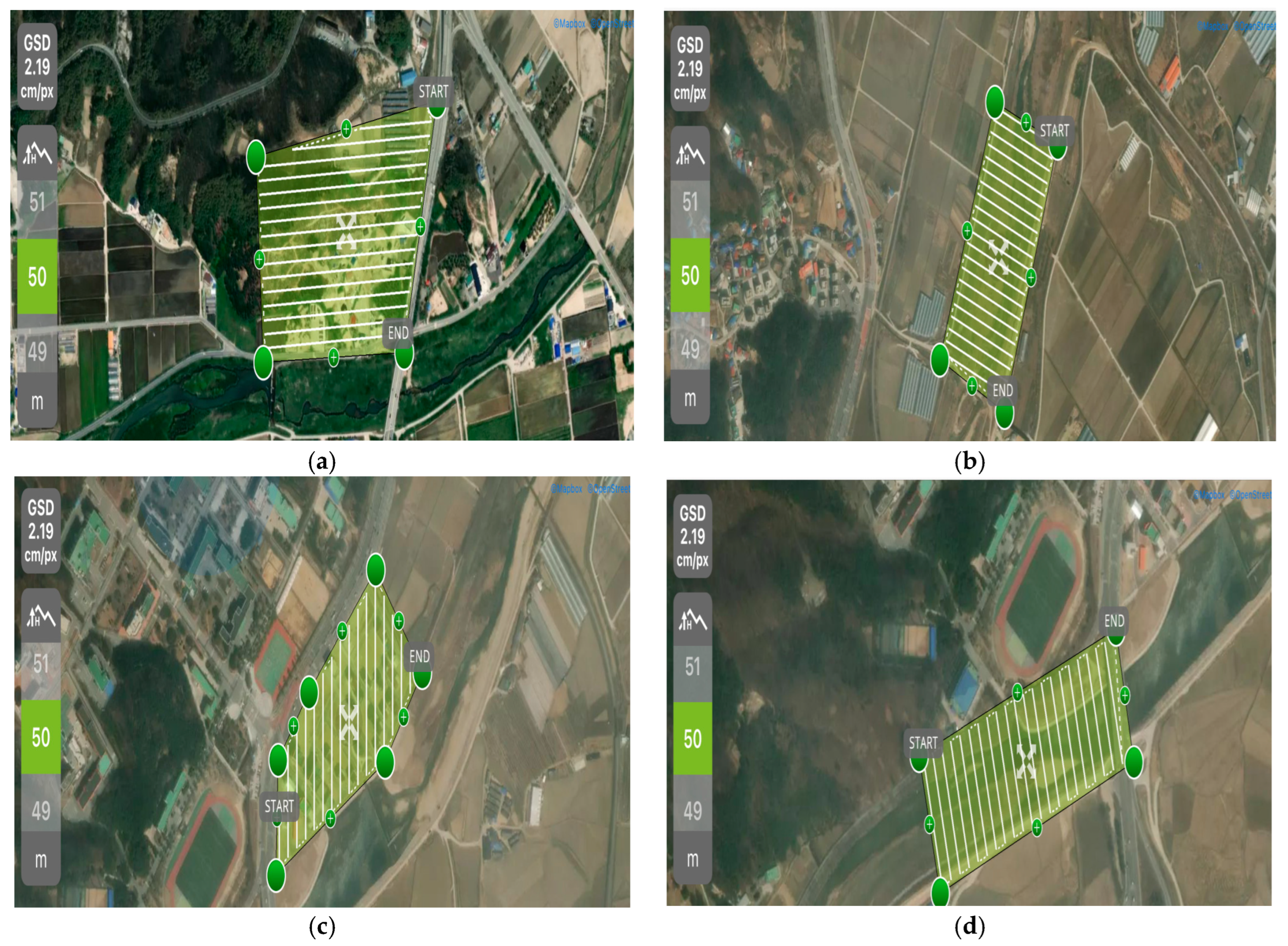
Figure 3 illustrates the flight plan for the study site and examples of RGB images. The other sensors acquired images by setting the same flight plan and data and setting the shooting altitude to 50 m, with 80% longitudinal and side overlap and 2–3 m/s flight speed. For the RGB sensor, research site A captured 162 images, site B captured 155 images, site C captured 170 images, and site D captured 143 images. As for the TIR sensor, site A acquired 334 images, site B acquired 312 images, site C acquired 354 images, and site D acquired 276 images. Figure 4 shows a part of a single image for each sensor acquired at study site A.
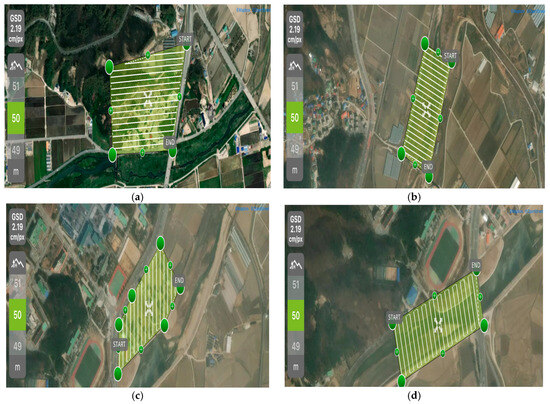
Figure 3.
Study area: (a) latitude: 38.234 and longitude: 128.570; (b) latitude: 36.375 and longitude: 128.147; (c) latitude: 36.377 and longitude: 128.149; and (d) latitude: 36.383 and longitude: 128.155.
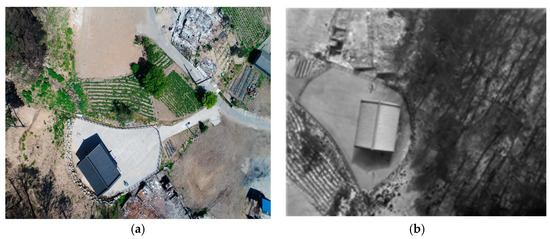
Figure 4.
Single image by sensor type for study area A: (a) RGB and (b) TIR.
2.2.2. GNSS Data Acquisition
The VRS survey is one of the network-RTK services provided by the NGII. The existing RTK survey requires two GNSS receivers used as the base and mobile stations, but the VRS survey can be conducted using a personal digital assistant (PDA) or a tablet PC capable of wireless communication with one GNSS receiver. As of August 2023, the VRS survey has been using a reference station comprising 92 GNSS regular observation stations (i.e., satellite reference points) nationwide. The VRS survey uses a network-RTK correction signal to obtain accurate positional data from a single GNSS receiver. The position correction values are transmitted to the mobile station to ensure high accuracy, compensating for errors caused by atmospheric conditions [17,18]. The L1C/A, L1C, L2C, L2E, and L5 signals from 12 to 15 GPS satellites were acquired during the survey. The average horizontal accuracy was 0.008 m, and the vertical accuracy was 0.009 m, with a PDOP ranging from 1.5 to 2.0. However, it is important to note that these values were achieved under favorable conditions, and the actual accuracy in typical field conditions may vary. Previous studies suggest that horizontal accuracy can typically range between 2–4 cm, and vertical accuracy may range from 2 to 3.5 cm, depending on factors such as PDOP and signal availability. The position dilution of the precision values was six or less and complied with network-RTK surveying regulation no. 2019-153 in the Public Surveying Work Regulations (NGII, Republic of Korea) [19]. According to this regulation, a minimum of 9 GCPs is required for a 1 km² area, and the number of CPs must be at least one-third of the GCPs, with a minimum of 3 CPs. The study area ranged from 0.04 km² to 0.08 km², meaning that 5 GCPs were sufficient under this regulation. Likewise, the use of 4 CPs met the minimum requirements for areas of this size. As a result of VRS acquisition, 5 GCPs were acquired for study area A, B, and D, 8 were acquired for study area C, and 4 CPs were acquired for all four study sites.
3. Method
3.1. RGB Orthophoto Generation
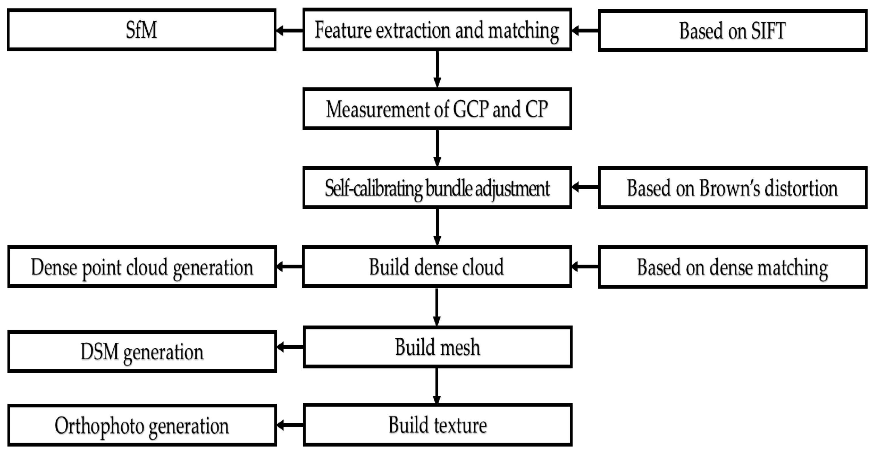
Figure 5 shows that the generation of the reference orthophoto using RGB images involves image alignment, feature point extraction, measurement of GCPs and CPs in the images, camera distortion correction, and the construction of a high-density point cloud, mesh model, and texture.
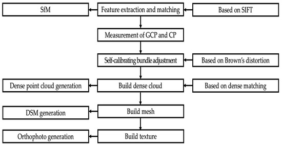
Figure 5.
RGB sensor image-processing flow.
The Agisoft Metashape software (version 1.6.3 Saint Petersburg, Russia) was used for the orthophoto generation process in this study. Although the algorithm used in Metashape is not officially documented, it operates in a manner similar to the scale-invariant feature transform (SIFT) method, which is commonly used for feature point extraction [20,21,22]. The SIFT method is a feature point extraction algorithm based on scale space [23], and it is designed to extract features that are invariant to changes in image size, rotation, and other factors. The method consists of the following four steps: scale space extrema detection, keypoint extraction, orientation assignment, and keypoint descriptor generation. After aligning the images, the bundle block adjustment process is performed. This process adjusts the relative positions and orientations of the images more accurately, resulting in improved camera orientation parameters and object coordinates for tie points. The object coordinates of tie points obtained from the bundle block adjustment are then used to generate a high-density point cloud. This is typically done through a process known as dense matching, where spatial coordinates for each pixel of the images are generated [24,25,26]. Camera distortion correction was also performed, which is an important factor in photogrammetry [27]. This correction was required after feature point extraction and before registration, as a distorted lens affects measurement accuracy. Camera distortion compensation uses Brown’s distortion model to optimize the camera calibration parameters [Equations (1)–(6)].
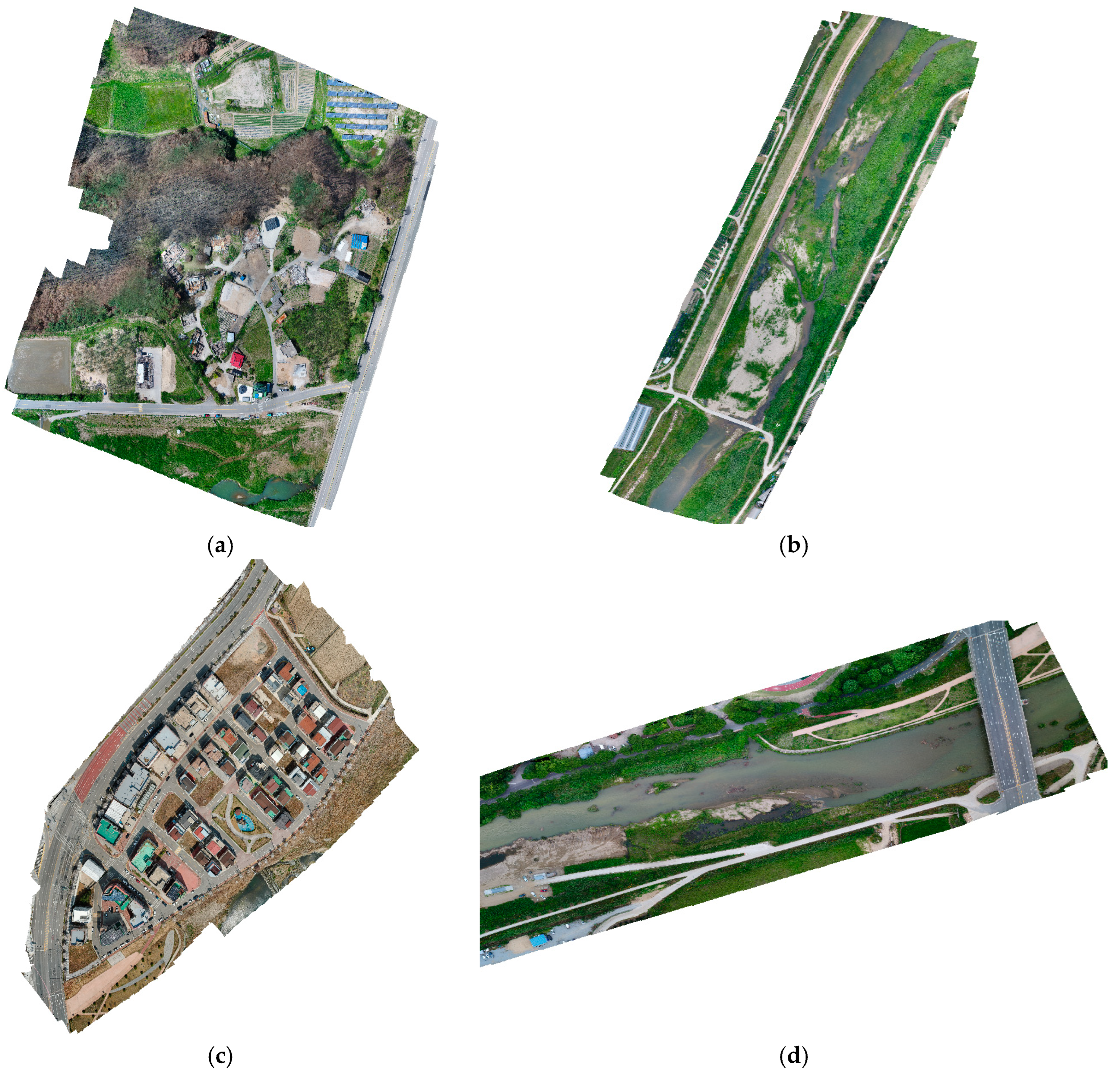
where X, Y, and Z are the point coordinates in the local camera coordinate system; u and v are the projected point coordinates in the image coordinate system (in pixels); f is the focal length; Cx and Cy are the principal point offsets; K1, K2, K3, and K4 are the radial distortion coefficients; P1 and P2 are the tangential distortion coefficients; B1 and B2 are the affinity and non-orthogonality coefficients, respectively; and w and h are the image width and height, respectively. Brown’s distortion model was used to correct the lens distortion in digital photography and multispectral cameras [28]. The feature points extracted based on the SIFT method proceeded with a high-density point construction through the structure from motion (SfM). The final orthophoto was generated after the mesh construction and texturing (Figure 6).

Figure 6.
Orthophotos of the four study areas: (a) latitude: 38.234 and longitude: 128.570; (b) latitude: 36.375 and longitude: 128.147; (c) latitude: 36.377 and longitude: 128.149; and (d) latitude: 36.383 and longitude: 128.155.
The accuracy of the orthophotos was evaluated using the CPs. Table 2 presents the root mean square error (RMSE) and the maximum error for the X and Y coordinates of the test points for each study site. The accuracy of the generated orthophotos was evaluated based on the Aerial Photogrammetry Work Regulation No. 2020-5165, Chapter 4, Article 50 of the Limitations of Adjustment Calculations and Errors, as stipulated by the NGII (Table 3). The RMSE and maximum tolerance for the RGB orthophotos across the four regions met the tolerance criteria for maps with a ground sample distance (GSD) of 8 cm. A geometric correction study was conducted using the accurate orthophotos generated with a GSD of 8 cm. The spatial resolution of all four study sites was approximately 2 cm.
Table 2.
Checkpoint RMSE and maximum error (unit: m).
Table 3.
Limitations of the adjustment calculations and errors stipulated by the NGII.
3.2. TIR Orthophoto Generation
3.2.1. TIR Orthophoto Generation (Zenmuse XT)
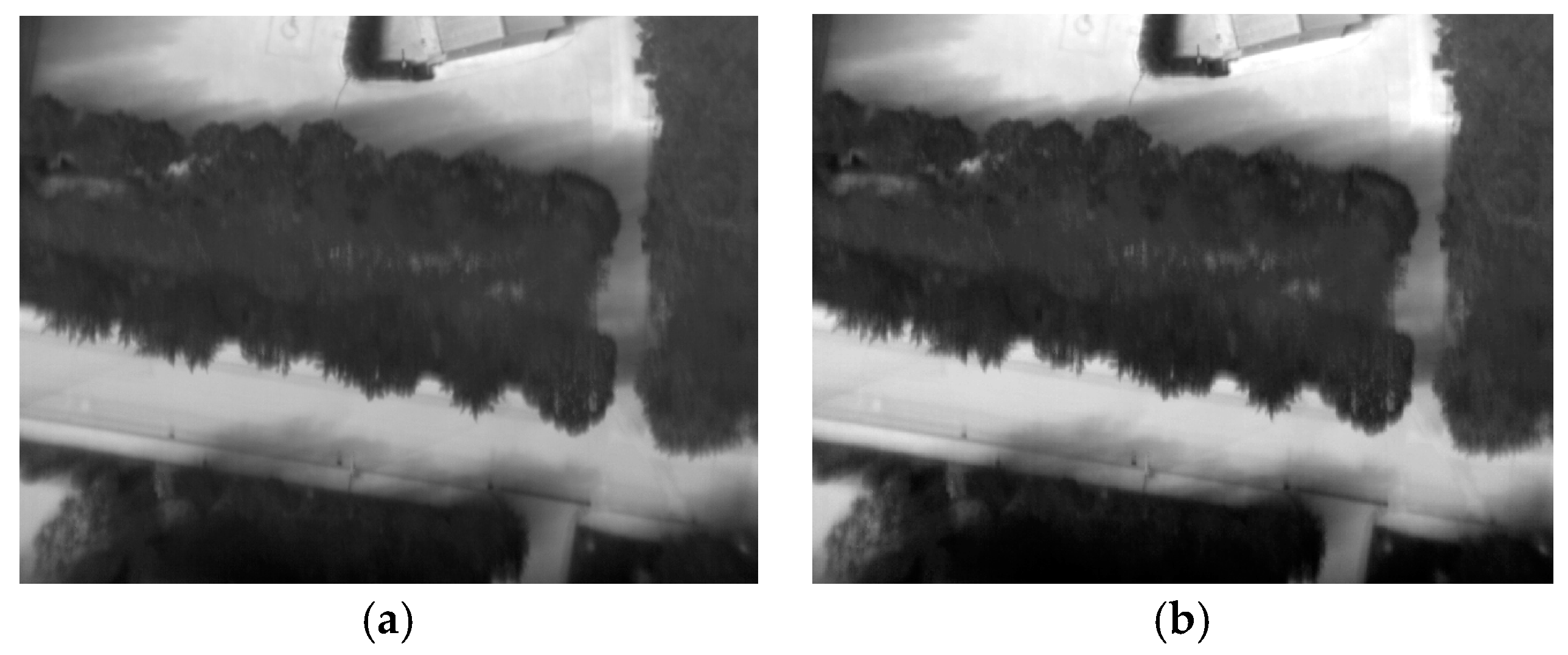
A TIR sensor used without pre- and post-processing is displayed as a digital number (DN) value instead of a Celsius temperature value; hence, the conversion from a joint photographic experts group (JPEG) file to a tagged image file format (TIFF) and the Celsius temperature conversion process are required. MATLAB (version 2022b), DJI Thermal SDK, and ExifTool software (version 12.42) were used for the pre- and post-processing of the TIR images. An 8-bit JPEG image was then converted into a 16-bit TIFF image to increase the precision of the thermal data. The 8-bit format only allows 256 levels of intensity, which limits the ability to capture subtle variations in thermal values. By converting to a 16-bit TIFF format, the image can represent 65,536 levels of intensity, allowing for much finer differentiation between temperature values. This conversion ensures that the subsequent thermal data processing and temperature calculations are more accurate and reliable. The conversion was performed using the metadata of the JPEG image and the -rawthermalimage-b command in the ExifTool via MATLAB (Figure 7). The single TIR image converted to a TIFF image was processed in the same manner as the RGB orthophoto generation process, except for the process of measuring the GCPs in the images through Metashape software (version 1.6.3). The generated orthophoto was still in DN values; thus, the 16-bit TIFF produced still contains DN values, and Equations (7)–(12) were used to convert these DN values into temperature in degrees Celsius. The parameters in the following formula vary depending on the TIR camera type and the external environment at the time of shooting [29,30]:

Figure 7.
Preprocessing process for TIR images: (a) 8 bit TIR image before conversion; (b) 16 bit TIR image after conversion.
The parameter information for the TIR sensor required , , , , , , , , , and [31]. These parameters were the unique values stored for each sensor to calculate the atmospheric attenuation. The information was stored as the TIR image metadata during shooting. The ExifToolGUI software (version 5.16) can extract EXIF information, and this was used to extract these values from the metadata. Table 4 presents the parameters. Equations (7)–(12) and the parameters listed in the table were calculated using MATLAB2022b and converted to land surface temperature (LST) orthophotos (Figure 8).
Table 4.
Parameters for the TIR sensor and environments (7) to (12).
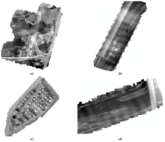
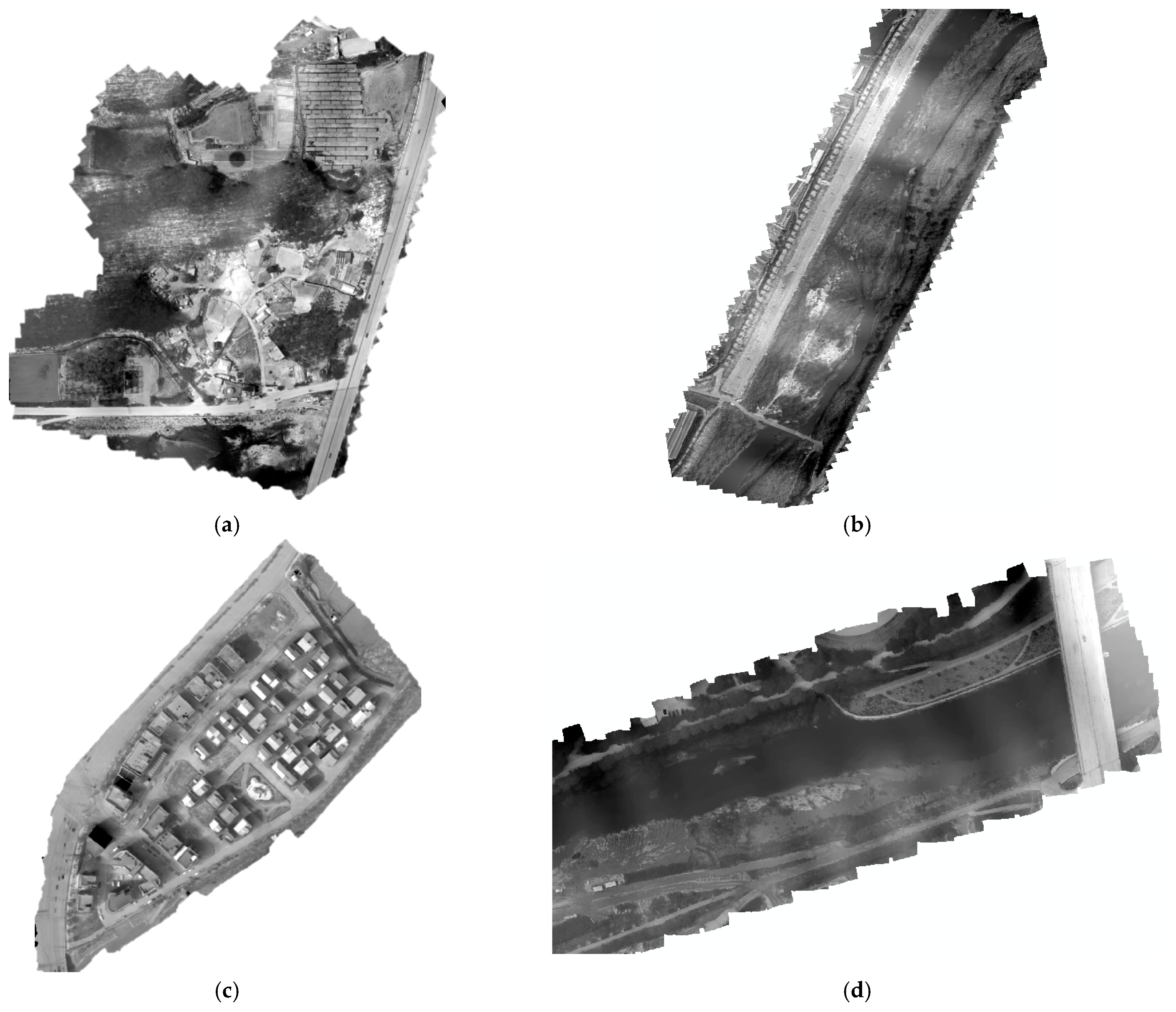
Figure 8.
TIR orthophotos of the four study areas (by Zenmuse XT): (a) latitude: 38.234 and longitude: 128.570; (b) latitude: 36.375 and longitude: 128.147; (c) latitude: 36.377 and longitude: 128.149; and (d) latitude: 36.383 and longitude: 128.155.
3.2.2. TIR Orthophoto Generation (Zenmuse H20T)
The TIR images acquired through the Zenmuse H20T, like those from the Zenmuse XT, are stored in an 8-bit JPEG format, where the data are represented as DN rather than direct temperature values. These DN values can be converted into temperature values. To generate LST orthophotos from Zenmuse H20T images, the JPEG images must be converted to TIFF format. This conversion can be performed using the DJI Thermal SDK and ExifTool with the appropriate parameters such as emissivity, humidity, and distance. Unlike the Zenmuse XT, the TIR image files from the Zenmuse H20T are expressed as temperature values after TIFF conversion. When the converted TIFF images are used to generate orthomosaics through Metashape, they are immediately expressed as LST orthophotos (Figure 9). The spatial resolution of the TIR orthophoto was around 6 cm, and resampling was performed to match the spatial resolution with the RGB orthophoto, reducing it from 6 cm to 2 cm. Feature point extraction was then carried out after the resampling process.
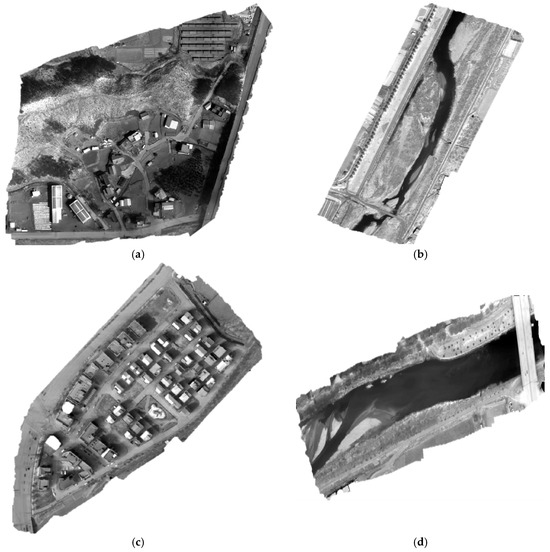
Figure 9.
TIR orthophotos of the four study areas (by Zenmuse H20T): (a) latitude: 38.234 and longitude: 128.570; (b) latitude: 36.375 and longitude: 128.147; (c) latitude: 36.377 and longitude: 128.149; and (d) latitude: 36.383 and longitude: 128.155.
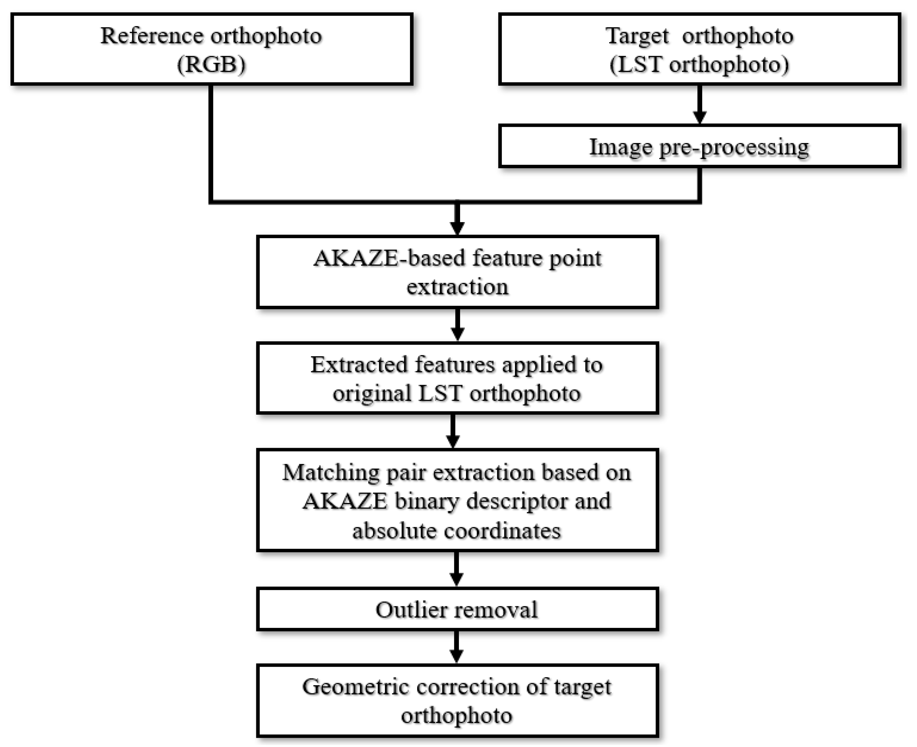
3.3. Geometric Correction between Orthophotos
Figure 10 shows the research flow chart for the geometric correction of orthophotos generated from RGB images and TIR sensor data. First, preprocessing was necessary for the TIR orthophotos because the small differences in pixel values between neighboring pixels made it difficult to extract features for accurate alignment. To address this issue, brightness-preserving BBHE and sharpening methods were applied to enhance feature extraction. The extracted features were then applied back to the original LST orthophotos before performing geometric correction, ensuring that the temperature values were not affected.

Figure 10.
Flow chart of the geometric correction on the optical orthophoto and the TIR orthophotos.
After preprocessing, feature points were extracted using the AKAZE method to match the positional relationships between the reference (RGB) and target (TIR) orthophotos. Only feature points with a scale of 2 or higher were extracted to reduce the computation load. Feature point matching was then performed, and outliers were removed using the RANSAC method and an iterative process to discard pairs with large RMSE values. Finally, geometric correction was applied using the affine transformation model to align the TIR orthophotos with the reference RGB images.
3.3.1. Preprocessing
For the TIR-generated temperature orthophoto, extracting features required for geometric correction was challenging because the differences in pixel values were minimal, making preprocessing necessary. Preprocessing was performed to extract more feature points compared to the original image by compensating for the brightness value distribution, allowing for better feature point matching. However, histogram equalization (HE) had the drawback of excessively altering the average brightness value of the transformed image compared to the original. Regardless of whether the average brightness value of the original image was high or low, HE transformed it to a mid-range contrast value, which led to an overemphasis on the brightness of the converted image [32]. In contrast, the BBHE method divided the average brightness value of the original image into two sub-histograms to avoid drastically changing the image brightness. Histogram smoothing was performed independently within each sub-histogram [33,34]. Using the BBHE method, additional sharpening was applied to enhance the image boundary, resulting in the extraction of more feature points compared to when only the BBHE method was used. The unsharp masking method was employed. Unsharp masking enhances sharpness by isolating the high-frequency components of the original image and adding them back to the image [35]. When the original and high-frequency images are combined, the edges are emphasized, and an image with improved contrast is obtained. The unsharp masking method is expressed by Equation (13) [36].
is the contrast enhancement result image with edge emphasis. is the input image. is the edge image for the contrast enhancement, which is the difference between the original and edge images.
A high-frequency image is obtained by using a Gaussian filter for the edge image. The blurring intensity can be adjusted with a constant that determines the Gaussian function shape through Equation (15) [37].
3.3.2. Feature Point Extraction (AKAZE)
The existing feature point extraction methods frequently use the SIFT and speeded up robust features (SURF) methods. The SURF method requires less computation than the SIFT method, making it widely used for feature point extraction during geometric correction [38,39]. Ultra-high-resolution orthophotos generated using UAV images contain various features. However, using a Gaussian filter, as in SIFT or SURF, can blur edges and corners, making accurate feature point extraction difficult [40]. The disadvantage of using a Gaussian filter is that it cannot effectively remove noise when generating a scale structure. Meanwhile, ultra-high-resolution orthophotos generated from UAV images can represent diverse topographies and features, such as roads, rocks, bare trees, and leaves, but feature point extraction is often hampered by the Gaussian filter [41]. To address these limitations, various methods such as binary robust invariant scalable keypoints (BRISK), oriented FAST and rotated BRIEF (ORB), KAZE, and AKAZE have been developed. The KAZE and AKAZE methods use a nonlinear diffusion filter to detect features in a nonlinear scale space, solving the unnatural contour problem that occurs with Gaussian filters [42,43]. It shows multi-scale performance with higher repeatability and identifiability than previous algorithms based on the Gaussian scale-space of SIFT and SURF [44]. For the AKAZE method, no analytical technique can be used to solve the nonlinear diffusion equation, which is a disadvantage of the existing KAZE method. Therefore, a numerical approach must be employed to approximate the solution. The KAZE method uses additive operator splitting for this purpose; however, it has the drawback of slow computation due to the large number of linear equations that must be solved to address the nonlinear diffusion equation. In contrast, the AKAZE method increases operation speed by utilizing a more advanced mathematical structure called fast explicit diffusion (FED). Additionally, the modified local-difference binary (M-LDB) descriptor is used to ensure efficient storage and low computational requirements [45,46,47].
The M-LDB descriptor, which is a modification of the local-difference binary (LDB) descriptor, is employed in the feature description process. To ensure a rotationally invariant descriptor, the grid is subsampled using a feature-dependent function, rather than taking the average value of all pixels in each grid subdivision. Representative information is extracted from each grid unit, and a binary test operation is performed on pairs of grid units. Upon completion of the AKAZE feature description step, a 61-dimensional descriptor is obtained.
3.3.3. Feature Matching
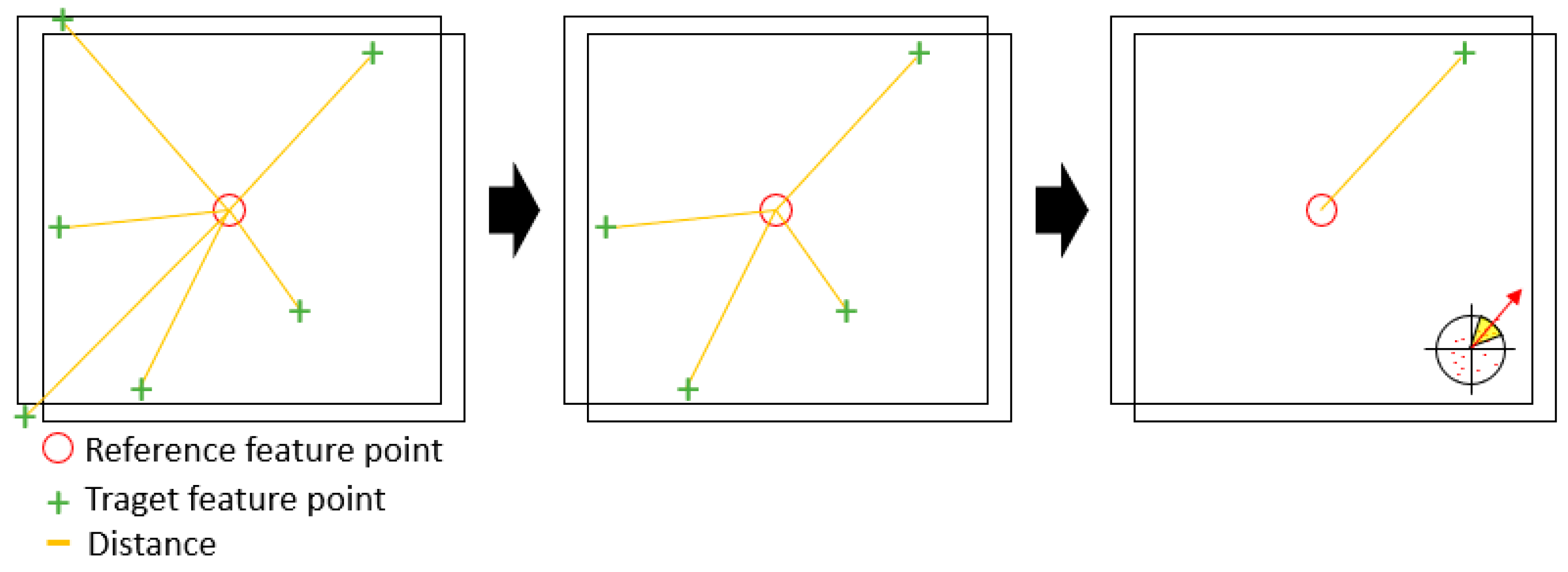
Matching pair extraction employs two methods: binary descriptor-based and coordinate-based methods. A descriptor that characterizes the feature points extracted by the AKAZE method must be created, and these characteristics are described using the generated descriptor. The AKAZE method utilizes a binary descriptor [48]. Various types of binary descriptors are also used in BRIEF, ORB, and BRISK feature point extraction methods. The M-LDB, which uses gradient and intensity information in the nonlinear scale space, was employed in the AKAZE method. The M-LDB used binary tests between area averages instead of individual pixels. In addition to the intensity value, the average values of the horizontal and vertical rates of change in the comparison area were also used, enabling the use of 3-bit information in the area comparison. The similarity of matched pairs was determined using the Hamming distance [49]. For feature points extracted by the AKAZE method, matching pairs were first extracted using binary descriptors. However, when matching pairs were extracted using only binary descriptors, they were not evenly distributed across the entire orthophoto. Therefore, matching pair extraction was necessary for feature points that were not matched using binary descriptors alone. The matching was performed by calculating the distance based on the coordinate difference between the reference and target orthophotos. The distance between neighboring feature points in the target orthophoto was calculated based on one feature point in the reference orthophoto. Candidates were selected such that the distance matched the feature point in the target orthophoto that fell within the threshold value. During the extraction of a candidate group of matching pairs, if one feature point matched multiple feature points in the target orthophoto, only one matching pair was allowed, considering directionality (Figure 11). The NGII aerial photogrammetry work regulations and the digital aerial photogrammetry adjustment calculations and margins of error were used to determine the threshold value. A matching pair extracted based on the final coordinates was fused with the previously obtained binary descriptor to determine the final matching pair.
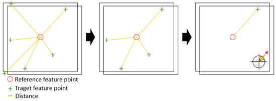
Figure 11.
Matching pair extraction based on coordinates.
3.3.4. Outlier Removal and Affine Transformation
The RANSAC method is widely used to remove outliers in geometric correction [50]. In RANSAC, a model equation that satisfies a matching pair is constructed after a random selection of sample data. The final model equation is selected when a matching pair that satisfies the model is estimated.
Affine transformation includes linear and translational transformations that preserve parallel lines in space. It can represent the relationships among rotation, shear, scale, inversion, and translation. The affine transformation model is expressed in Equation (16). Six coefficients are calculated for the construction of the affine transformation model, and at least three matching pairs are required to calculate these six coefficients. However, more than three matching pairs can be calculated using the least squares method [51].
4. Results and Discussion
4.1. Application of Geometric Correction
In this work, many feature points were extracted by compensating for the brightness value distribution using the BBHE method. Preprocessing was also performed to ensure good matching. Subsequently, a sharpening method was applied to improve boundary contrast, resulting in more feature points being extracted compared to when only the BBHE method was used (Table 5). The BBHE and sharpening methods efficiently extracted feature points from the LST orthophoto.
Table 5.
Number of feature points of the TIR orthophoto according to preprocessing.
Feature point extraction for the preprocessed image was performed using the AKAZE method. Compared to SIFT, SURF, ORB, and BRISK, which are widely used in existing feature point extraction approaches, the AKAZE method is one of the most efficient in terms of overall speed, number of feature points, and matching pairs (Table 6). Although AKAZE extracts fewer feature points than SIFT when applied to a single image, it offers higher accuracy relative to time. It also performs well in low-illumination images, allowing for effective feature point extraction even in terrains with varying elevations. AKAZE is particularly effective for orthophotos from UAVs operating at different altitudes [52]. A comparison of the results from study sites B and D shows that ORB seems to be the best in terms of speed and feature point extraction; however, the number of matching pairs is significantly lower than that of other methods. In summary, AKAZE is the most effective method when considering both time and the number of feature points.
Table 6.
Number of feature points extracted and the required time.
After extracting feature points using the AKAZE method, the first matching pair was extracted using a binary descriptor. First, the nearest and second nearest neighbors were identified. The ratio of the nearest neighbor to the second nearest neighbor was then calculated for each feature descriptor. Matching items were filtered based on a specific critical ratio. The coordinate-based distance difference between the reference and target orthophotos was calculated, and matching pairs were extracted. Subsequently, matching pair candidates were selected by setting a threshold value based on the UAV survey work regulation for digital aerial photogrammetry adjustment calculations and error limits for the distance difference. When multiple feature points were matched to a single feature point, only one matching pair was extracted, considering directionality. RANSAC was used to remove outliers and obtain precise matching pair results.
Figure 12 presents the results of outlier removal using only binary descriptors. Figure 13 shows the results of outlier removal by applying our proposed method.
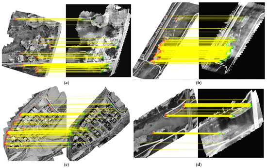
Figure 12.
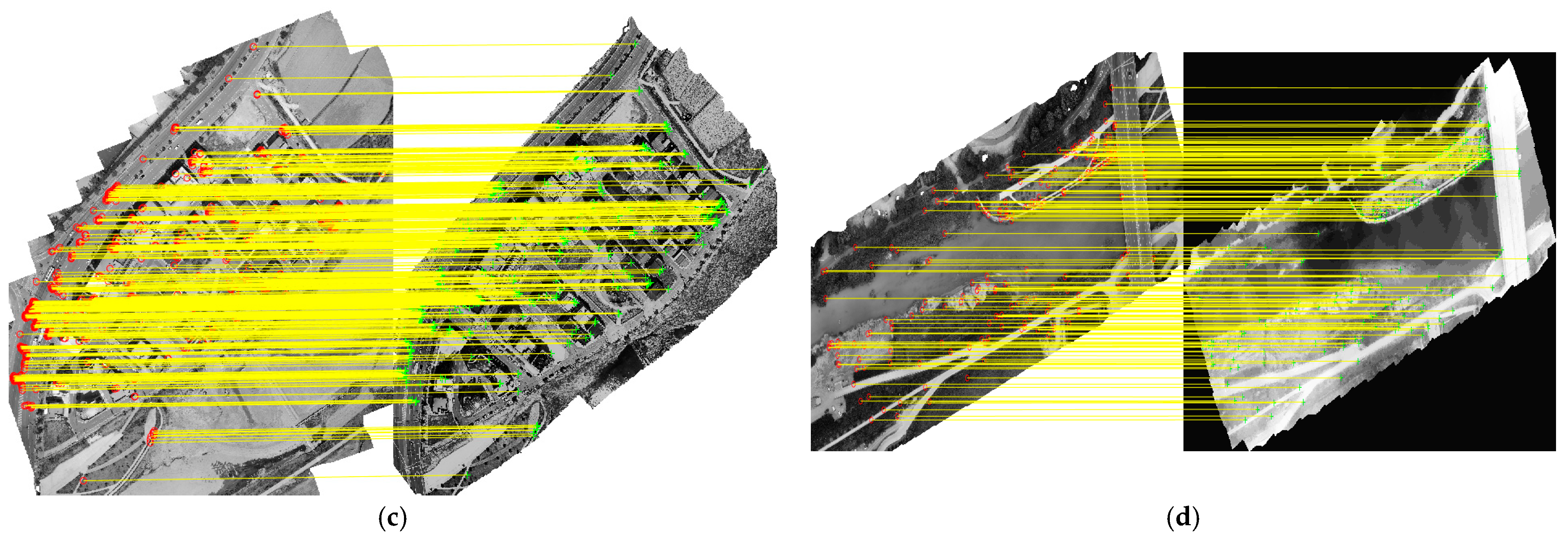
Result of the TIR mismatching pair removal in the four study areas (by the binary descriptor): (a) left: 3 September 2019 and right: 3 September 2019; (b) left: 23 June 2019 and right: 15 December 2019; (c) left: 28 April 2020 and right: 17 May 2020; and (d) left: 1 July 2019 and right: 9 July 2019. The red points represent the feature points of the reference image, the green points represent the feature points of the target image, and the yellow lines indicate the matching pairs.

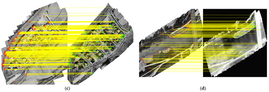
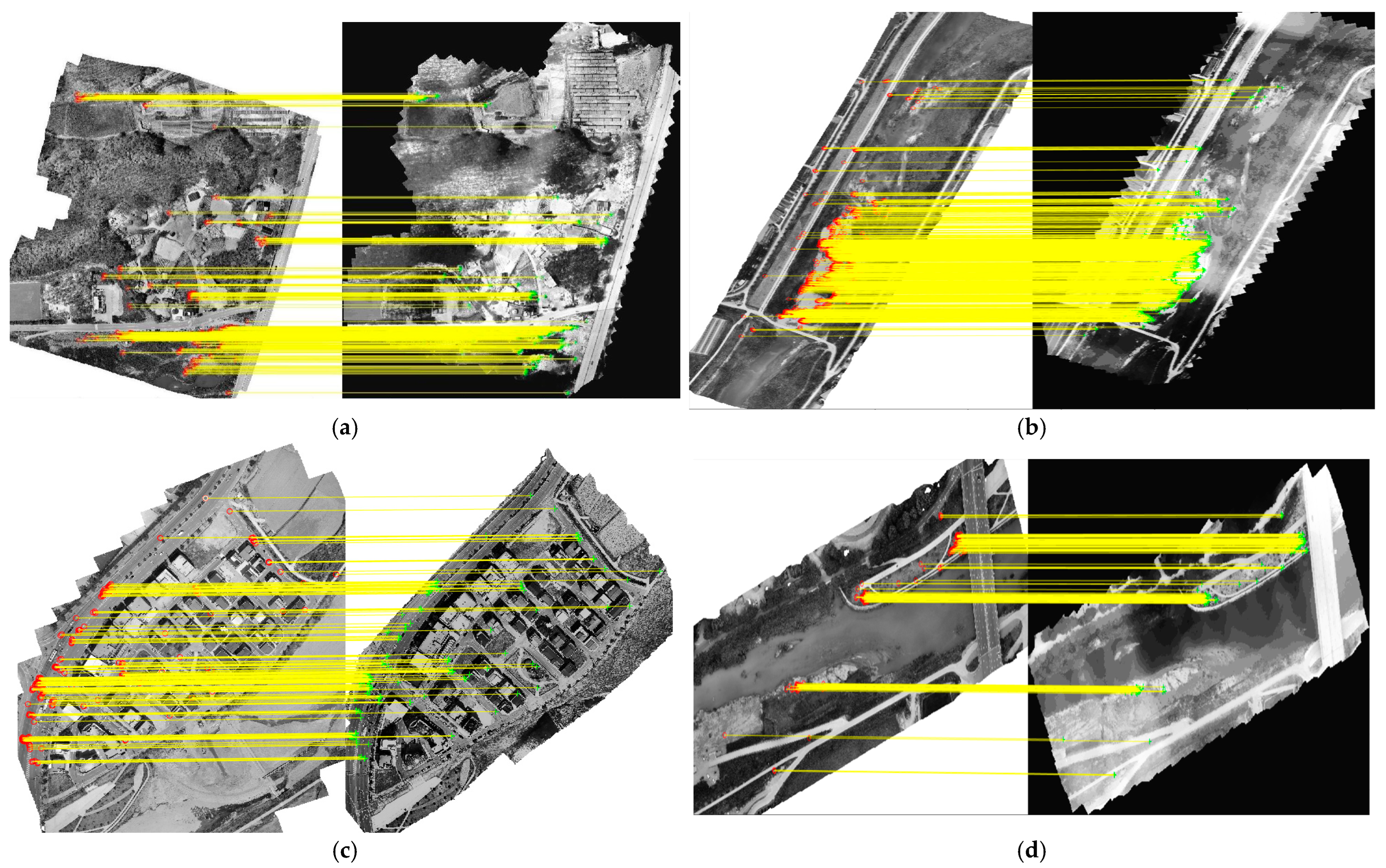
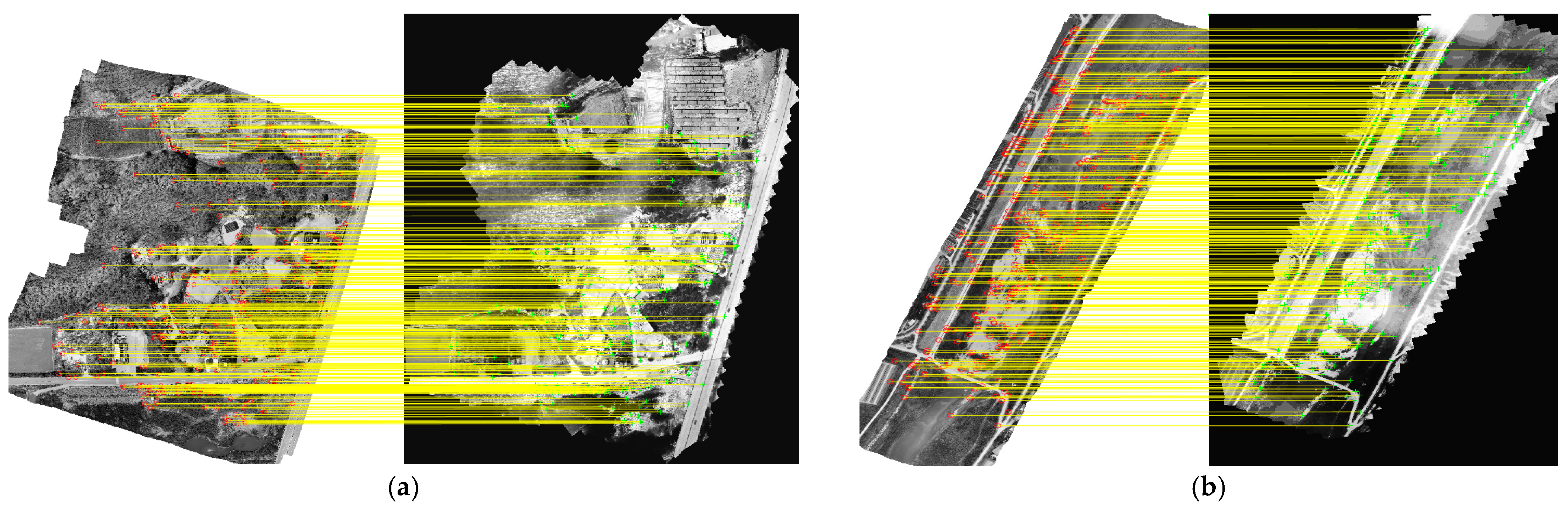
Figure 13.
Result of the TIR mismatching pair removal in the four study areas (by the distance and direction method): (a) left: 3 September 2019 and right: 3 September 2019; (b) left: 23 June 2019 and right: 15 December 2019; (c) left: 28 April 2020 and right: 17 May 2020; and (d) left: 1 July 2019 and right: 9 July 2019. The red points represent the feature points of the reference image, the green points represent the feature points of the target image, and the yellow lines indicate the matching pairs.
The outlier removal results using RANSAC showed that when only binary descriptors were used, study site A had 380 matches, B had 440, C had 386, and D had 171. Using the proposed technique, study site A had 454 matches, B had 486, C had 492, and D had 221 (Table 7). When matching pairs were extracted using the proposed technique, both the number of matching pairs and their distribution across the image increased. Figure 14 illustrates the geometric correction results with the matching pairs extracted using the proposed technique and an overlapping mosaic image, created by dividing the reference and target images into a grid format.
Table 7.
Outlier removal results using RANSAC.
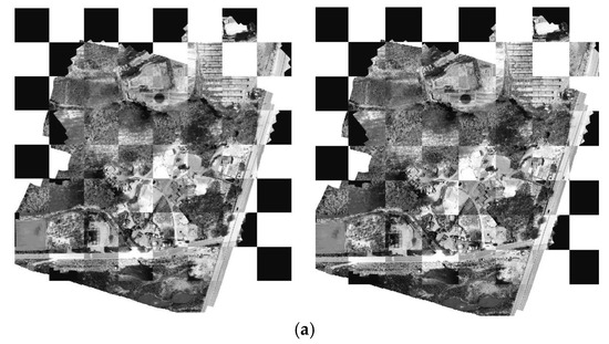
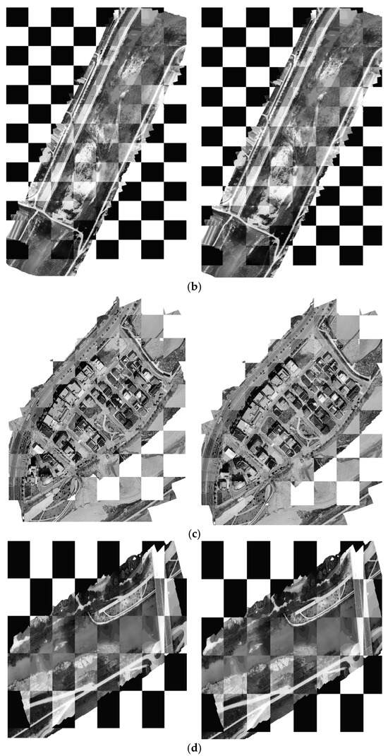
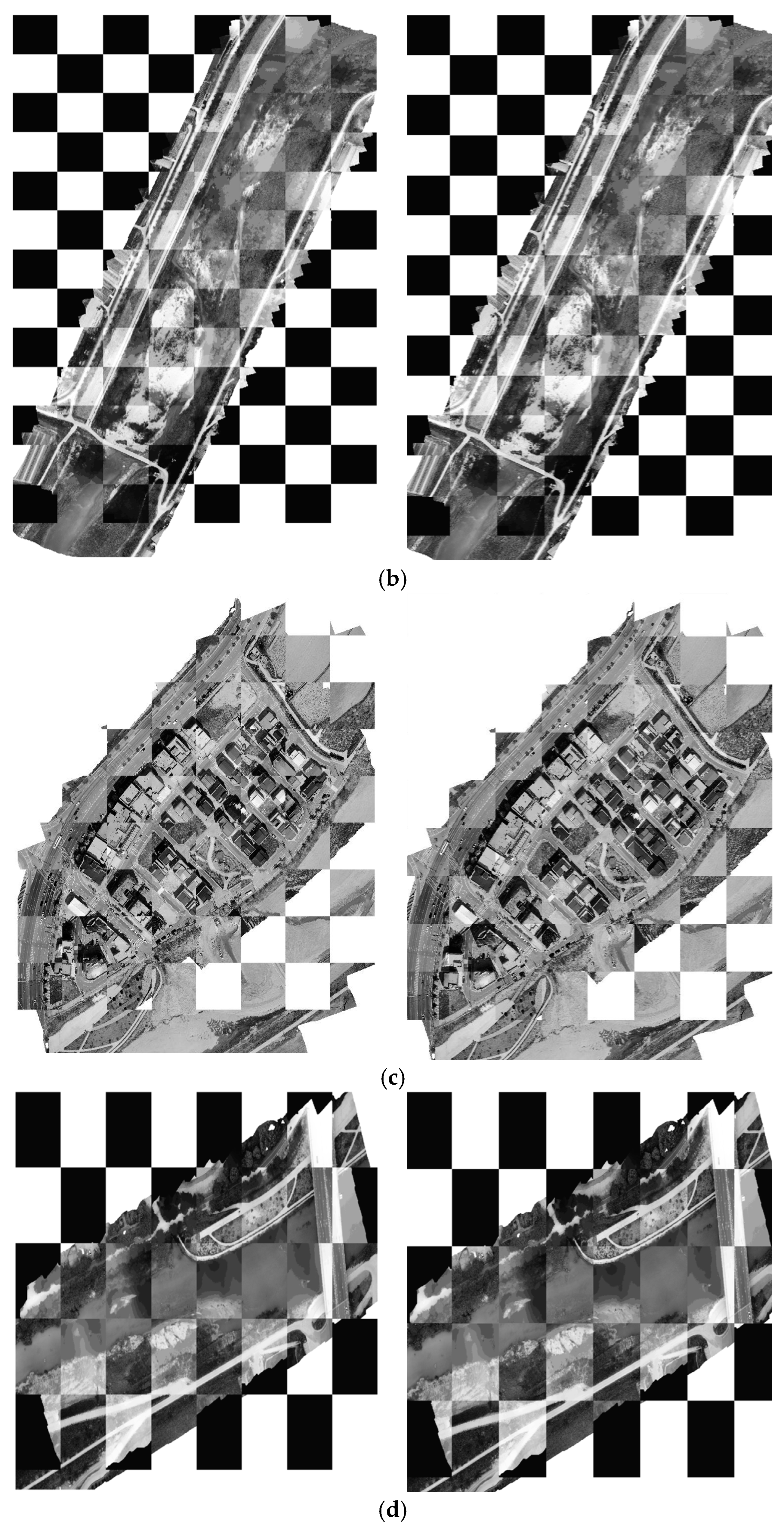
Figure 14.
Result of the mosaic image after performing the geometric correction for the TIR (left: original orthophotos; right: geometry correction orthophotos): (a) left: 3 September 2019 and right: 3 September 2019; (b) left: 23 June 2019 and right: 15 December 2019; (c) left: 28 April 2020 and right: 17 May 2020; and (d) left: 1 July 2019 and right: 9 July 2019.
4.2. LST Orthophoto Correction Results
Table 8 shows the results of correctly matched pairs (inliers) in the TIR temperature orthophoto. Figure 15 displays a visual inspection of the mosaic image after the geometric correction for each study area. In the LST orthophotos, matching pairs were not extracted from roads and lanes with invariant characteristics. The surface temperature of roads was higher than that of other types of land cover because the materials used were concrete or asphalt. In other words, matching pairs were not efficiently selected in the case of the LST orthophotos. These characteristics confirmed that geometric correction works well when a topography or feature among the elements has consistent characteristics or remains invariant in the LST orthophoto when using the existing method. However, the lack of distinct and consistent features across the images makes it difficult to find matching pairs, which in turn complicates the geometric correction process. Except for study site C, all study sites were areas that underwent many changes over time. However, on 30 March 2023, at study site C, the inlier count decreased compared to other times due to the unexpected presence of shadows during the acquisition of a single TIR image, despite acquiring the image near noon to minimize shadow effects. The results revealed that the number of inliers was small when only binary descriptors were used for the orthophotos with large time differences. By contrast, the proposed method could identify more inliers.
Table 8.
Overall results of the TIR orthophoto geometric correction by study area.
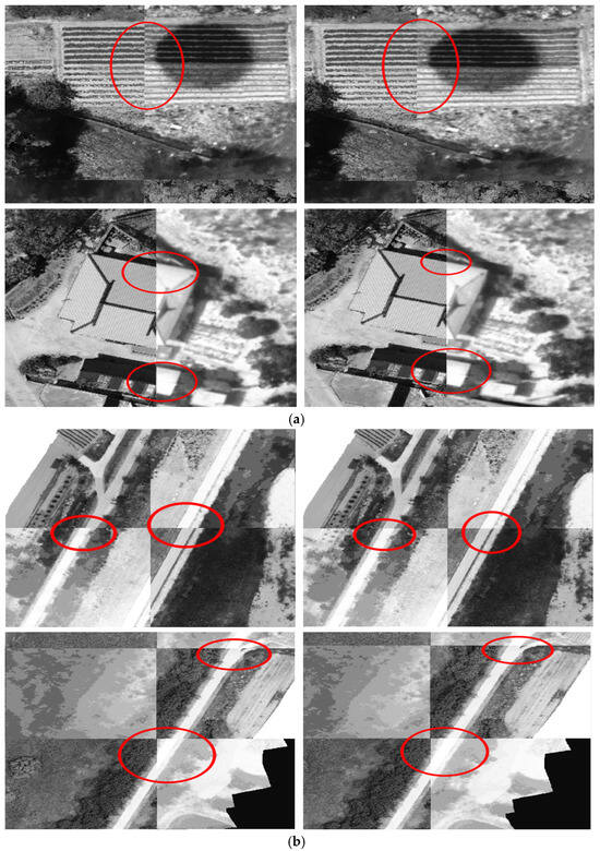
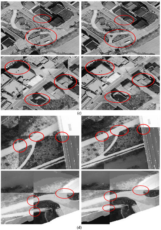
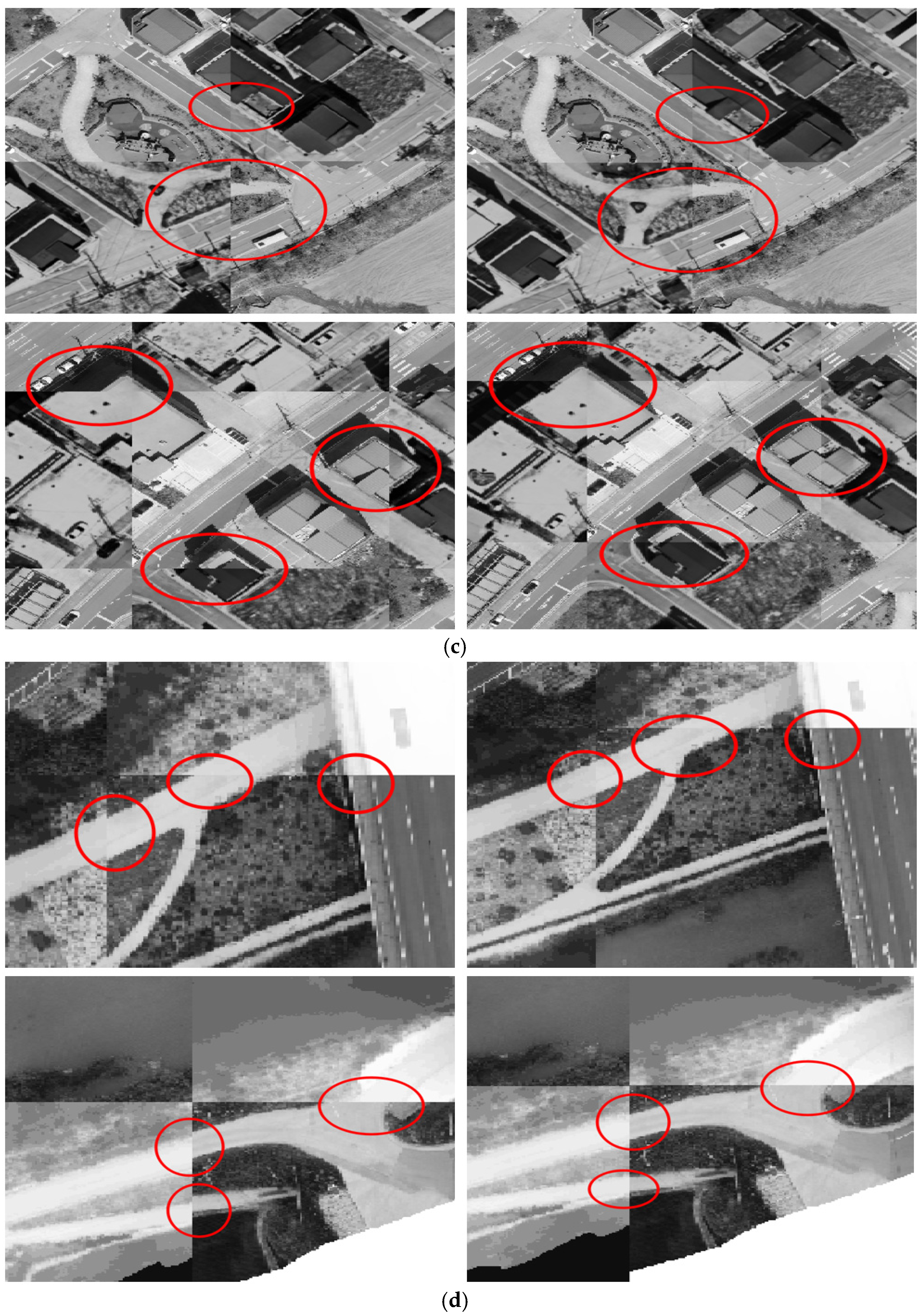
Figure 15.
Visual inspection of TIR orthophoto mosaic images before and after geometric correction for each study area (enlarged image before correction on the left, enlarged image after correction on the right).: (a) left: 3 September 2019 and right: 3 September 2019; (b) left: 23 June 2019 and right: 15 December 2019; (c) left: 28 April 2020 and right: 17 May 2020; and (d) left: 1 July 2019 and right: 9 July 2019.
4.3. Quantitative Evaluation
Table 9 shows the pixel and coordinate-based differences before and after geometric correction of the LST orthophoto. For study points A~D, the pixel difference before geometric correction was at least 5 px (0.10 m) and at most 30 px (0.60 m). After geometric correction, the existing method showed a difference of 0.7~5 px (0.01~0.10 m), and geometric correction was not possible in some cases. However, the proposed method was able to perform geometric correction, which was not possible in the existing method, and showed a difference of 0.7~7 px (0.01~0.14 m). In the case of the existing method, geometric correction was not possible when there was a change or time difference. However, the proposed method performed geometric correction with a difference of about 5~7 px (0.10~0.14 m) compared to a difference of 9~25 px (0.18~0.50 m) in the area where geometric correction was not possible in the existing method. In the case of the orthophoto at a time point where geometric correction was not possible in the existing method, the proposed method satisfied the digital aerial photography GSD standard of 12 cm (19 April 2023 and 6 March 2021) or 25 cm (18 March 2023 and 19 March 2023). The orthophoto at the time geometric correction was possible and met the 8cm digital aerial photography GSD standard.
Table 9.
Quantitative evaluation (RMSE) of the TIR orthophotos (pixel/m).
5. Conclusions
This study aimed to perform accurate geometric correction of the orthophotos for the sensors used by reducing the errors that may occur during the input process and addressing the disadvantage of the large amount of time required for surveying and measuring GCPs in the images.
A comparison of the SIFT, SURF, ORB, BRISK, and AKAZE methods for feature point extraction confirmed that AKAZE is more effective in extracting feature points relative to time in the orthophotos of all the sensors used. Matching features was more difficult when only existing binary descriptors were used because similarities were not obtained in the matching process, even if many feature points were extracted in regions with significant changes over time. In contrast, the proposed method was able to extract matching pairs in regions with unequal similarity, resulting in more matching pairs than when only binary descriptors were used and performing geometric correction more effectively across the entire orthophoto compared to existing methods.
Orthophotos must be periodically produced using UAVs for various sensors. When generating orthophotos with accurate location coordinates, challenges such as interruptions in RTK UAV reception or difficulty in locating GCPs in certain sensor data can arise. Our proposed method helps correct uncorrected imagery caused by these issues, ensuring accurate geometric correction even in cases where RTK signals are lost or GCPs cannot be easily detected. When the abovementioned situation occurs, the geometric correction between different sensors can be performed using reference RGB orthophotos. The resolution of a single TIR image was very low compared to that in other sensors, making it difficult to measure the GCP image coordinates for each image. Although measuring the GCP image coordinates is time-consuming, this study demonstrates that geometric correction can be successfully achieved using the reference orthophoto, providing a reliable alternative to traditional GCP-based methods. Correspondingly, precise orthophotos can be generated by performing a time-efficient geometric correction, reducing the reliance on extensive GCP measurements and providing an effective supplementary method for cases where GCPs are not readily available. Future research should investigate the feature point and matching pair extraction process that is robust to topography and feature characteristics using deep learning, particularly for areas that undergo significant changes. Additionally, research is needed on the efficient removal of mismatched pairs and the application of geometric correction to sensors other than TIR sensors.
Author Contributions
Conceptualization, K.L.; methodology, W.L.; software, K.L.; formal analysis, W.L. and K.L.; writing—original draft preparation, K.L.; writing—review and editing W.L.; funding acquisition, W.L. All authors have read and agreed to the published version of the manuscript.
Funding
This research was supported by the Basic Science Research Program through the National Research Foundation of Korea (NRF) funded by the Ministry of Education (NRF-2020R1I1A3061750 and RS-2023-00274068) and a National Research Foundation of Korea (NRF) grant funded by the Korean government (MSIT) (no. NRF-2021R1A5A8033165).
Data Availability Statement
Dataset available on request from the authors.
Acknowledgments
The authors wish to acknowledge the Research Institute of Artificial Intelligent Diagnosis Technology for Multi-scale Organic and Inorganic Structure, Kyungpook National University, Sangju, Republic of Korea, for providing laboratory facilities.
Conflicts of Interest
The authors declare no conflicts of interest.
References
- Stöcker, C.; Nex, F.; Koeva, M.; Gerke, M. High-quality uav-based orthophotos for cadastral mapping: Guidance for optimal flight configurations. Remote Sens. 2020, 12, 3625. [Google Scholar] [CrossRef]
- Deliry, S.I.; Avdan, U. Accuracy of unmanned aerial systems photogrammetry and structure from motion in surveying and mapping: A review. J. Indian Soc. Remote Sens. 2021, 49, 1997–2017. [Google Scholar] [CrossRef]
- Liu, Y.; Zheng, X.; Ai, G.; Zhang, Y.; Zuo, Y. Generating a high-precision true digital orthophoto map based on UAV images. ISPRS Int. J. Geo-Inf. 2018, 7, 333. [Google Scholar] [CrossRef]
- Kovanič, Ľ.; Topitzer, B.; Peťovský, P.; Blišťan, P.; Gergeľová, M.B.; Blišťanová, M. Review of photogrammetric and lidar applications of UAV. Appl. Sci. 2023, 13, 6732. [Google Scholar] [CrossRef]
- Attard, M.R.; Phillips, R.A.; Bowler, E.; Clarke, P.J.; Cubaynes, H.; Johnston, D.W.; Fretwell, P.T. Review of Satellite Remote Sensing and Unoccupied Aircraft Systems for Counting Wildlife on Land. Remote Sens. 2024, 16, 627. [Google Scholar] [CrossRef]
- Li, H.; Yin, J.; Jiao, L. An Improved 3D Reconstruction Method for Satellite Images Based on Generative Adversarial Network Image Enhancement. Appl. Sci. 2024, 14, 7177. [Google Scholar] [CrossRef]
- Gudžius, P.; Kurasova, O.; Darulis, V.; Filatovas, E. Deep learning-based object recognition in multispectral satellite imagery for real-time applications. Mach. Vis. Appl. 2021, 32, 98. [Google Scholar] [CrossRef]
- Shoab, M.; Singh, V.K.; Ravibabu, M.V. High-precise true digital orthoimage generation and accuracy assessment based on UAV images. J. Indian Soc. Remote Sens. 2022, 50, 613–622. [Google Scholar] [CrossRef]
- Jang, H.; Kim, S.; Yoo, S.; Han, S.; Sohn, H. Feature matching combining radiometric and geometric characteristics of images, applied to oblique-and nadir-looking visible and TIR sensors of UAV imagery. Sensors 2021, 21, 4587. [Google Scholar] [CrossRef]
- Döpper, V.; Gränzig, T.; Kleinschmit, B.; Förster, M. Challenges in UAS-based TIR imagery processing: Image alignment and uncertainty quantification. Remote Sens. 2020, 12, 1552. [Google Scholar] [CrossRef]
- Park, J.H.; Lee, K.R.; Lee, W.H.; Han, Y.K. Generation of land surface temperature orthophoto and temperature accuracy analysis by land covers based on thermal infrared sensor mounted on unmanned aerial vehicle. J. Korean Soc. Surv. Geod. Photogramm. Cartogr. 2018, 36, 263–270. [Google Scholar]
- Shin, Y.; Lee, C.; Kim, E. Enhancing Real-Time Kinematic Relative Positioning for Unmanned Aerial Vehicles. Machines 2024, 12, 202. [Google Scholar] [CrossRef]
- Hognogi, G.G.; Pop, A.M.; Marian-Potra, A.C.; Someșfălean, T. The role of UAS-GIS in Digital Era Governance.A Systematic literature review. Sustainability 2021, 131, 11097. [Google Scholar] [CrossRef]
- Kim, S.; Lee, Y.; Lee, H. Applicability investigation of the PPK GNSS method in drone mapping. J. Korean Cadastre Inf. Assoc. 2021, 23, 155–165. [Google Scholar] [CrossRef]
- Seong, J.H.; Lee, K.R.; Han, Y.K.; Lee, W.H. Geometric correction of none-GCP UAV orthophoto using feature points of reference image. J. Korean Soc. Geospat. Inf. Syst. 2020, 27, 27–34. [Google Scholar]
- Angel, Y.; Turner, D.; Parkes, S.; Malbeteau, Y.; Lucieer, A.; McCabe, M.F. Automated georectification and mosaicking of UAV-based hyperspectral imagery from push-broom sensors. Remote Sens. 2019, 12, 34. [Google Scholar] [CrossRef]
- Son, J.; Yoon, W.; Kim, T.; Rhee, S. Iterative Precision Geometric Correction for High-Resolution Satellite Images. Korean J. Remote Sens. 2021, 37, 431–447. [Google Scholar]
- Chen, J.; Cheng, B.; Zhang, X.; Long, T.; Chen, B.; Wang, G.; Zhang, D. A TIR-visible automatic registration and geometric correction method for SDGSAT-1 thermal infrared image based on modified RIFT. Remote Sens. 2022, 14, 1393. [Google Scholar] [CrossRef]
- Li, Y.; He, L.; Ye, X.; Guo, D. Geometric correction algorithm of UAV remote sensing image for the emergency disaster. In Proceedings of the IEEE International Geoscience and Remote Sensing Symposium (IGARSS), Beijing, China, 10–15 July 2016; pp. 6691–6694. [Google Scholar]
- Dibs, H.; Hasab, H.A.; Jaber, H.S.; Al-Ansari, N. Automatic feature extraction and matching modelling for highly noise near-equatorial satellite images. Innov. Infrastruct. Solut. 2022, 7, 2. [Google Scholar] [CrossRef]
- Retscher, G. Accuracy performance of virtual reference station (VRS) networks. J. Glob. Position. Syst. 2002, 1, 40–47. [Google Scholar] [CrossRef]
- Wanninger, L. Virtual reference stations (VRS). Gps Solut. 2003, 7, 143–144. [Google Scholar] [CrossRef]
- Lee, K.; Lee, W.H. Earthwork Volume Calculation, 3D model generation, and comparative evaluation using vertical and high-oblique images acquired by unmanned aerial vehicles. Aerospace 2022, 9, 606. [Google Scholar] [CrossRef]
- Goncalves, J.A.; Henriques, R. UAV photogrammetry for topographic monitoring of coastal areas. ISPRS J. Photogramm. Remote Sens. 2015, 104, 101–111. [Google Scholar] [CrossRef]
- Reshetyuk, Y.; Mårtensson, S. Generation of highly accurate digital elevation models with unmanned aerial vehicles. Photogramm. Rec. 2016, 31, 143–165. [Google Scholar] [CrossRef]
- Hendrickx, H.; Vivero, S.; De Cock, L.; De Wit, B.; De Maeyer, P.; Lambiel, C.; Delaloye, R.; Nyssen, J.; Frankl, A. The reproducibility of SfM algorithms to produce detailed Digital Surface Models: The example of PhotoScan applied to a high-alpine rock glacier. Remote Sens. Lett. 2019, 10, 11–20. [Google Scholar] [CrossRef]
- Lowe, D.G. Distinctive image features from scale-invariant keypoints. Int. J. Comput. Vis. 2004, 60, 91–110. [Google Scholar] [CrossRef]
- Sun, Q.; Wang, X.; Xu, J.; Wang, L.; Zhang, H.; Yu, J.; Su, T.; Zhang, X.F. Camera Self-Calibration with Lens Distortion. Optik 2016, 127, 4506–4513. [Google Scholar] [CrossRef]
- Lee, W.H.; Yu, K. Bundle block adjustment with 3D natural cubic splines. Sensors 2009, 9, 9629–9665. [Google Scholar] [CrossRef]
- Lee, K.; Lee, W.H. Temperature accuracy analysis by land cover according to the angle of the thermal infrared imaging camera for unmanned aerial vehicles. ISPRS Int. J. Geo-Inf. 2022, 11, 204. [Google Scholar] [CrossRef]
- Jiang, J.; Zheng, H.; Ji, X.; Cheng, T.; Tian, Y.; Zhu, Y.; Cao, W.; Ehsani, R.; Yao, X. Analysis and evaluation of the image preprocessing process of a six-band multispectral camera mounted on an unmanned aerial vehicle for winter wheat monitoring. Sensors 2019, 19, 747. [Google Scholar] [CrossRef]
- Weng, J.; Zhou, W.; Ma, S.; Qi, P.; Zhong, J. Model-free lens distortion correction based on phase analysis of fringe-patterns. Sensors 2020, 21, 209. [Google Scholar] [CrossRef] [PubMed]
- Di Felice, F.; Mazzini, A.; Di Stefano, G.; Romeo, G. Drone high resolution infrared imaging of the Lusi mud eruption. Mar. Pet. Geol. 2018, 90, 38–51. [Google Scholar] [CrossRef]
- Lee, K.; Park, J.; Jung, S.; Lee, W. Roof Color-based warm roof evaluation in cold regions using a UAV mounted thermal infrared imaging camera. Energies 2021, 14, 6488. [Google Scholar] [CrossRef]
- Aubrecht, D.M.; Helliker, B.R.; Goulden, M.L.; Roberts, D.A.; Still, C.J.; Richardson, A.D. Continuous, long-term, high-frequency thermal imaging of vegetation: Uncertainties and recommended best practices. Agric. For. Meteorol. 2016, 228, 315–326. [Google Scholar] [CrossRef]
- Lu, L.; Zhou, Y.; Panetta, K.; Agaian, S. Comparative study of histogram equalization algorithms for image enhancement. In Proceedings of the Mobile Multimedia/Image Processing, Security, and Applications 2010, FL, USA, 5–9 April 2010; pp. 337–347. [Google Scholar]
- Acharya, U.K.; Kumar, S. Image sub-division and quadruple clipped adaptive histogram equalization (ISQCAHE) for low exposure image enhancement. Multidimension. Syst. Signal Process. 2023, 34, 25–45. [Google Scholar]
- Zhou, J.; Pang, L.; Zhang, W. Underwater image enhancement method based on color correction and three-interval histogram stretching. Meas. Sci. Tech. 2021, 32, 115405. [Google Scholar] [CrossRef]
- Kaur, S.; Kaur, M. Image sharpening using basic enhancement techniques. Int. J. Res. Eng Sci. Manag. 2018, 1, 122–126. [Google Scholar]
- Kim, H.G.; Lee, D.B.; Song, B.C. Adaptive Unsharp Masking using Bilateral Filter. J. Inst. Electron. Inf. Eng. 2012, 49, 56–63. [Google Scholar]
- Kansal, S.; Purwar, S.; Tripathi, R.K. Image contrast enhancement using unsharp masking and histogram equalization. Multimed. Tools Appl. 2018, 77, 26919–26938. [Google Scholar] [CrossRef]
- Devi, N.B.; Kavida, A.C.; Murugan, R. Feature extraction and object detection using fast-convolutional neural network for remote sensing satellite image. J. Indian Soc. Remote Sens. 2022, 50, 961–973. [Google Scholar] [CrossRef]
- Oh, J.; Han, Y. A double epipolar resampling approach to reliable conjugate point extraction for accurate Kompsat-3/3A stereo data processing. Remote Sens. 2020, 12, 2940. [Google Scholar] [CrossRef]
- Fortun, D.; Bouthemy, P.; Kervrann, C. Optical flow modeling and computation: A survey. Comput. Vis. Image Underst. 2015, 134, 1–21. [Google Scholar] [CrossRef]
- Gastal, E.S.; Oliveira, M.M. Domain transform for edge-aware image and video processing. In Proceedings of the ACM SIGGRAPH 2011, Vancouver, BC, Canada, 7–11 August 2011; pp. 1–12. [Google Scholar]
- Demchev, D.; Volkov, V.; Kazakov, E.; Alcantarilla, P.F.; Sandven, S.; Khmeleva, V. Sea ice drift tracking from sequential SAR images using accelerated-KAZE features. IEEE Trans. Geosci. Remote Sens. 2017, 55, 5174–5184. [Google Scholar] [CrossRef]
- Soleimani, P.; Capson, D.W.; Li, K.F. Real-time FPGA-based implementation of the AKAZE algorithm with nonlinear scale space generation using image partitioning. J. Real-Time Image Process. 2021, 18, 2123–2134. [Google Scholar] [CrossRef] [PubMed]
- Sharma, S.K.; Jain, K.; Shukla, A.K. A Comparative Analysis of Feature Detectors and Descriptors for Image Stitching. Appl. Sci. 2023, 13, 6015. [Google Scholar] [CrossRef]
- Alcantarilla, P.F.; Bartoli, A.; Davison, A.J. KAZE features. In Proceedings of the Computer Vision—ECCV 2012, Florence, Italy, 7–13 October 2012; pp. 214–227. [Google Scholar]
- Weickert, J.; Grewenig, S.; Schroers, C.; Bruhn, A. Cyclic schemes for PDE-based image analysis. Int. J. Comput. Vis. 2016, 118, 275–299. [Google Scholar] [CrossRef]
- Weickert, J.; Scharr, H. A scheme for coherence-enhancing diffusion filtering with optimized rotation invariance. J. Vis. Commun. Image Represent. 2002, 13, 103–118. [Google Scholar] [CrossRef]
- Hong, S.; Shin, H. Comparative performance analysis of feature detection and matching methods for lunar terrain images. KSCE J. Civ. Environ. Eng. Res. 2020, 40, 437–444. [Google Scholar]


Disclaimer/Publisher’s Note: The statements, opinions and data contained in all publications are solely those of the individual author(s) and contributor(s) and not of MDPI and/or the editor(s). MDPI and/or the editor(s) disclaim responsibility for any injury to people or property resulting from any ideas, methods, instructions or products referred to in the content. |
© 2024 by the authors. Licensee MDPI, Basel, Switzerland. This article is an open access article distributed under the terms and conditions of the Creative Commons Attribution (CC BY) license (https://creativecommons.org/licenses/by/4.0/).