0-D Dynamic Performance Simulation of Hydrogen-Fueled Turboshaft Engine

Abstract

In the last few decades, the problem of pollution resulting from human activities has pushed research toward zero or net-zero carbon solutions for transportation. The main objective of this paper is to perform a preliminary performance assessment of the use of hydrogen in conventional turbine engines for aeronautical applications. A 0-D dynamic model of the Allison 250 C-18 turboshaft engine was designed and validated using conventional aviation fuel (kerosene Jet A-1). A dedicated, experimental campaign covering the whole engine operating range was conducted to obtain the thermodynamic data for the main engine components: the compressor, lateral ducts, combustion chamber, high- and low-pressure turbines, and exhaust nozzle. A theoretical chemical combustion model based on the NASA-CEA database was used to account for the energy conversion process in the combustor and to obtain quantitative feedback from the model in terms of fuel consumption. Once the engine and the turbomachinery of the engine were characterized, the work focused on designing a 0-D dynamic engine model based on the engine’s characteristics and the experimental data using the MATLAB/Simulink environment, which is capable of replicating the real engine behavior. Then, the 0-D dynamic model was validated by the acquired data and used to predict the engine’s performance with a different throttle profile (close to realistic request profiles during flight). Finally, the 0-D dynamic engine model was used to predict the performance of the engine using hydrogen as the input of the theoretical combustion model. The outputs of simulations running conventional kerosene Jet A-1 and hydrogen using different throttle profiles were compared, showing up to a 64% reduction in fuel mass flow rate and a 3% increase in thermal efficiency using hydrogen in flight-like conditions. The results confirm the potential of hydrogen as a suitable alternative fuel for small turbine engines and aircraft.

1. Introduction

Mitigating the effects of climate change is one of the priorities of both global and national administrations, with far-reaching implications for the environment, economies, and societies worldwide. As is well known, climate change is primarily driven by human activities, notably the emission of greenhouse gases such as carbon dioxide, methane, and nitrous oxide. Since 1990, there has been a steady increase in anthropogenic emissions of greenhouse gases (GHGs), which is expected to continue to increase in future years exponentially [1]. From the combustion of fossil fuels to power cars, trucks, ships, and aircraft to its sprawling delivery infrastructures, the transportation sector is a major contributor to climate change. Currently, carbon dioxide (CO₂) emissions from the transportation sector account for about 30% of emissions in developed countries and approximately 23% of the total man-made CO₂ emissions worldwide [2]. As a result, governments and global organizations have redefined their agendas to promote sustainable technical solutions for the next generation of mobility [3,4,5] that are capable of addressing the carbon neutrality goals for the transportation sector. The guidelines proposed by the IEA (International Energy Agency) set several objectives to be reached by 2050 [6]. Among these, huge investments and research efforts have been focused on innovative zero or net-zero carbon fuels and vehicles aimed at driving this transition while saving the main technical characteristics of the existing engine technologies [7].

In this scenario, electric and hybrid vehicles are considered promising for ground transportation [8]. While electric propulsion has proven to be an efficient solution for ground vehicles, battery packs have serious drawbacks in other applications, especially in aviation, where size and weight requirements are critical. Therefore, sustainable aviation fuels (SAFs), including synthetic fuels, bio-fuels, and gaseous zero-carbon alternatives, such as hydrogen [7,9], have been proposed for the next generation of air mobility. The ever-increasing global demand for petroleum, which will increase the cost per mile and the need for cleaner high-energy carriers has increased the attention of the research community and aviation industries on the development of these solutions.

Bio-fuels are typically derived from organic matter, mainly from plants or organic wastes, with different manufacturing processes depending on the primary source. M.H.B. Tajuddin. et al. [10] tested Jatropa-based bio-fuel in the Allison 250 gas turbine engine with good performance results, and confirmed its potential as a possible candidate to replace conventional fossil fuels. However, biofuels are not a fully viable solution to decrease GHG emissions because they still retain a percentage of environmentally harmful gases, which are generated by the combustion of molecules containing carbon (carbon dioxide, carbon monoxide, hydrocarbon chains). On the other hand, synthetic fuels (or e-fuels) are typically produced by coupling electrochemical processes, such as carbon capture, hydrolysis, and Fisher-Tropsch, using renewable energy sources [11]. Despite the fact that running e-fuels in conventional aviation engines, i.e., pistons and turbine engines, does not prevent the generation of engine-out emissions, the e-fuels production route better allows for reaching the zero-carbon footprint goal compared to bio-fuels [11]. The third player in the green transition of aviation from a fuel technology perspective is hydrogen. Although molecular hydrogen (H₂) is quite rare in the Earth’s atmosphere, atomic hydrogen (H) is largely abundant in other composites, such as water (H₂O) and methane (CH₄), and can be extracted in different ways (hydrolysis, steam reforming). This offers a clear competitive edge to address the ever-increasing energy demand in future years. Moreover, due to its extremely high energy density (120 MJ/kg) and the lack of carbon atoms, hydrogen represents a viable candidate to effectively replace fossil fuels for both transportation and power generation [12,13,14,15].

Despite these advantages, the low density of hydrogen, along with its gaseous state, poses the greatest challenges to the handling, delivery, and combustion of hydrogen in conventional aircraft engines. Compared to biofuels and e-fuels, both of which are easily stored as a liquid at atmospheric pressure in conventional tanks, hydrogen has much different requirements in terms of onboard storage and ground facilities. H. Degirmenci et al. [16] demonstrated that the conversion of hydrogen production and delivery infrastructure in airports can be achievable without decreasing their effectiveness. On the other hand, the on-board storage of hydrogen is considered the main challenge in aviation due to its chemical characteristics. Several studies have been carried out to explore different portable hydrogen storage solutions, including high-pressure tanks, metal hydrides storage, and cryogenic tanks [17].

In addition to on-board H₂ storage systems, propulsion architectures have also received a great deal of research attention in recent years, and various configurations are currently under investigation. Among the others, two are the technical solutions that have shown the most benefits: burning H₂ in conventional engines, or an integrated electric propulsion system based on a fuel-cell (H₂-FC) genset and electric motors. The use of H₂-FC fuel cells is particularly interesting because it can be considered 100% pollutant-free (only water vapors are present at the FC outlet). In addition, coupling FC with electric motors in an integrated green propulsion unit promotes a clear advance in the MOA (More Electric Aircraft) program, one of the main development trends in the air mobility industry [18,19].

Although the advantages of H₂-FC are undisputedly recognized, their applications on aircraft also have drawbacks. The major limitations of FC technologies are their low power-to-weight ratio, which is one of the key decision drivers for aviation applications, and the need for an efficient cooling system (with big heat exchangers that cannot be easily installed on board), which is known to be crucial for FC efficiency and durability optimization [20,21]. In this field, a lot of research is currently ongoing on high-temperature fuel cells (FC-HT) that may lead to attaining such a solution suitable for aircraft [22].

As mentioned before, operating H₂ in conventional aeronautical engines is considered a valuable alternative to FC in decarbonizing the aviation sector. The most diffused engines in aviation are turbine engines with all their variants. Many studies in the literature have advanced the feasibility of hydrogen conversion for conventional turbine engines. Different aspects of this engine conversion have been thoroughly investigated, such as the mechanical and chemical compatibility of standard fuel lines and components with hydrogen, combustion chamber cooling and design, and engine performance and reliability.

In the early 2000s, some studies proposed innovative combustion chamber designs that promote stable hydrogen combustion in conventional engine platforms [23,24]. A. Adam et al. [25] demonstrated that handling an extremely light gaseous fuel such as hydrogen requires a different approach to the injection system design compared to liquid fuels. Due to its very high flame speed and high energy density, hydrogen needs injection systems and combustion chamber designs that enhance the mixing of fuel and air in a small volume. Among others, H. H.-W. Funke et al. [26] and A. Haj Ayed et al. [27] proposed the so-called “micro-mix system”, demonstrating that a proper system and injection design can guarantee good combustion efficiency and low production of NOx. In the “micro-mix” combustion system, the flame is kept stable on an injection plate with a pattern of miniaturized injectors. The small dimension of the injectors and their uniform spatial distribution prevent the formation of big flames (with a consequent local increase in temperature). Moreover, the generation of small combustion surfaces allows for decreasing the overall dimensions of the combustion chamber and reducing NO_X production.

Most of the new configurations developed for turbine engines are still under development or undergoing a long process of testing due to the extremely high reliability level required for aeronautical applications. For this reason, even though new solutions enabling hydrogen combustion have been widely studied in recent years, the market penetration of these technologies is delayed by the certification and approval process [28], which increases the cost. As a result, the research on this new technology is being accompanied by the development of numerical models that allow for obtaining data with less investments in time and resources. In the field of hydrogen technology for turbine engines, the numerical models developed in the past can be divided into two main categories: (i) thermo-fluid dynamic models of components, typically used to study in detail the behavior of single phenomena in engine components; (ii) simplified thermodynamic models of the propulsion system. Some examples are reported in recent studies carried out by A. Adam et al. [25] and A.H. Ayed et al. [27], respectively.

Despite some assumptions, complete engine models have proven to be accurate enough to describe and evaluate the potential and performance of new solutions in existing and previously validated HGs in aviation. A simplified theoretical chemical combustion model based on the NASA-CEA database was considered aimed at obtaining a quantitative estimation of thermal efficiency and fuel flow rate during standard operating conditions. Several studies focused on the development of this kind of model: H. R. Babahammou et al. [29] simulated the combustion of natural gas blended with hydrogen in a gas turbine using Aspen HYSYS software simulator and compared the results obtained with the different mixtures, defining the advantages in global emissions achievable by mixing hydrogen with conventional fuels; O. Balli et al. [30] performed a thermodynamic analysis aimed at underlining the differences between the use of kerosene and hydrogen in a turbofan engine, defining in detail the exegetic and energetic parameters of the two fuels; X. Wang et al. [31] simulated with both Simulink and Speedgoat-based hardware in the loop system the dynamic behavior of multiple hydrogen-fed aeronautical engines under development, assessing the advantages with regards to hydrogen combustion.

The purpose of this paper is to perform a preliminary performance evaluation of a hydrogen-fueled turbine engine through dynamic 0-D simulations. The numerical model of the engine, a conventional Allison 250 C-18 turboshaft engine, was developed using information provided by the engine manufacturer and experimental measurements. This model is based on a previous study performed by F. Ponti et al. [32] on the same engine. The field is still open to the development of new models, extending the analysis over different engine architectures, and exploiting innovative strategies aimed at the final objective of reducing emissions from air transportation. Then, the model was validated in the typical engine operating range using experimental data acquired in a test cell running kerosene Jet A-1. Once validated, the model was converted to run on hydrogen and a preliminary performance analysis in different engine conditions was conducted. Typical mission profiles were tested running on kerosene and H₂ and the main engine parameters were compared. The results obtained from the simulations demonstrated that, together with evident reductions in fuel mass flow rate related to the different LHVs of hydrogen, improvements in thermal efficiency were also achieved.

2. Materials and Methods

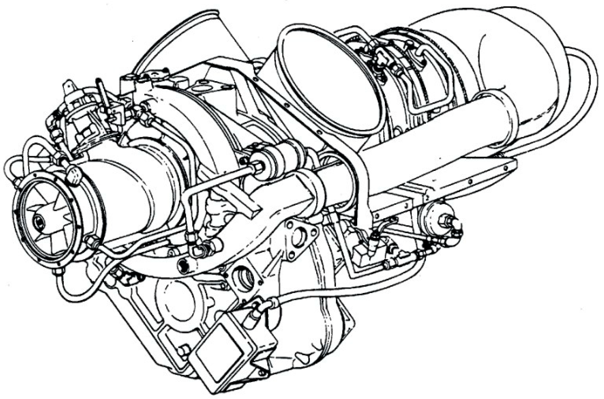
2.1. Engine Description

The engine selected in this work is the Allison 250 C-18, a small, mechanically actuated turboshaft engine for small aircraft and helicopters. The M250 family has a very large array of models, all sharing a similar modular design: twin shaft architecture with a two-stage LPT, a two-stage HPT, and a gearbox with a gear rate of 5.83. All the models also share a reverse-flow combustion chamber with exhaust pipes in the mid-section of the engine [33,34]. The main characteristics of the engine are described in

Table 1. Engine technical characteristics [35].

Engine Parameter	Values
Engine Type	Double-shaft turbine engine
Compressor Type	6 axial stages and 1 centrifugal stage
Gas generator Turbine Type	2 axial stages
Power Turbine Type	2 axial stages
Combustion Chamber Type	Single Body Three-staged with Reverse Flow
Maximum Torque	338 Nm @ Take-Off
Maximum Power	201 kW @ Maximum Continuous Power at Sea Level
Injection System	Single–entry Dual–orifice Type Unit
Control System	Hydromechanical
Compression ratio	6.2:1
Gas Generator Shaft Speed at 100%	51,120 rpm
Output Shaft Speed at 100%	6000 rpm
Weight	64 kg @ Dry
Dimensions	1026 × 483 × 572 mm

.

The main feature of this engine is the single-body reverse-flow combustion chamber. As is visible in Figure 1, the design and dimensions of the engine guarantee a very compact shape, suitable for small aircraft. The air received from the intake is firstly processed by the 6 Axial Compressor Stages (ACSs) and later by the single Centrifugal Compressor Stage (CCS). Both the ACSs and the CCS rotor components are mechanically connected to the Gas Generator (GG) shaft as a single body. The compressed air obtained is then redirected to the end of the motor through two peripherical pipes outside the CCS to the Combustion Chamber (CC). Thanks to the CC’s internal geometry, the air enters the combustion chamber gradually along its length, ensuring a quasi-stoichiometric combustion inside the main volume and promoting the air–fuel mixing. The fuel is introduced into the CC through a center-mounted single injector next to an aerospace spark igniter. The combustion chamber is schematically divided into three main zones: the Primary Combustion Zone (PCZ), the Secondary Combustion Zone (SCZ), and the Mixing Zone (MZ). The PCZ, located in the first section of the CC along with the fuel injector and igniter, is the area where the largest portion of the fuel (up to 80%) participates in the combustion process with the primary air flow. In the SCZ, the section of the CC after the PCZ, additional air enters the CC, sustaining the combustion reaction with the remaining fuel. Finally, the MZ is the last section of the CC and is designed to maximize the mixing between combustion products and the remaining air, and to reduce the temperature of the exhaust gases before they enter the turbines.

As mentioned above, this engine is characterized by the presence of two independent turbines, each consisting of two axial stages: the High-Pressure Turbine (HPT) drives the compressor, while the Low-Pressure Turbine (LPT), mounted after the HPT in the flow path, is connected on a secondary power shaft which enters the gearbox. The turbomachines and the main engine components are shown in Figure 2 [35,36].

As is usual in turbine engine design, the engine can be divided into two main sections based on the chemical composition and temperature of the flow: the cold section and the hot section. The cold section starts from the inlet and runs down to the CC inlet (only fresh air is present in this zone), while the hot section begins from the CC up to the engine exhaust (where hot exhaust gases can be found). Inside the combustion chamber, the main flow (primary air and fuel) is diluted with the secondary mass flow that enters the engine, and the chemical composition of the exhaust gas flow (function of temperature, pressure, and relative percentage of reactants—air and fuel) is drastically modified by the combustion that occurs subsequently. The geometry of the entire engine and its components—obtained from the literature and from direct measurements—is used to design the 0-D dynamic model [35,36].

This engine is a good representation of a large array of aeronautical engines used in general aviation, and the results obtained studying this engine could be easily extended to similar models. The choice of such an engine provides this study with a vast field of application, ranging from general aviation helicopters to common commercial airliners, promoting the transition towards sustainable fuels of a significant number of aircraft.

2.2. Fuel Properties and Chemical Equilibrium Calculation

As previously mentioned, to obtain quantitative results in terms of fuel consumption and BSFC, a simplified combustion chamber was considered within the engine model. A theoretical chemical combustion model based on the CEA-Run database was implemented, and the thermodynamic properties of the exhaust gases from the combustion model were used in the hot section of the model both for the fossil fuel (kerosene Jet A-1) and the sustainable fuel (gaseous hydrogen) considered in this work. The main properties of Jet A-1 and hydrogen at atmospheric pressure (on the ground, 1 bar) and 15 degrees Celsius (288.14 K) are listed in

Table 2. Benchmarking of the fuels properties used in this work [37,38,39].

Fuel	Molar Weight, M [kg*kmol−1]	Lower Heating Value, LHV [kJ*kg−1]	Density [kg*m−3]
Jet A-1	167.314	43.28	802.8
Hydrogen	2.016	119.45	0.083

.

As can be noticed, hydrogen has a much higher Lower Heating Value (LHV) compared to Jet A-1 (119.45 kJ*kg⁻¹ compared to 43.28 kJ*kg⁻¹), and a much lower density (4 orders of magnitude of difference). These features are considered the most promising characteristics of hydrogen supply, but do not directly indicate an increase in engine performance due to the complex hydrogen combustion mechanism and the interaction between the turbomachines.

The CEA-Run database [40,41] contains all the information needed to calculate the chemical equilibrium during combustion when using different fuels. Although the tool used to simulate the combustion process provides feedback of complete (100% of fuel is burned) and instantaneous combustion chemical reactions, the large amount of air that flows within the combustion chamber, along with the length of the liner, leads to considering the distance between the real and the ideal combustion process as negligible for the scope of this work. This assumption has also been confirmed by the comparison of experimental data (pressure and temperature at the combustion chamber outlet) and the output of the CEA-Run model, considering the ambient atmospheric pressure and 15 °C as thermodynamic conditions of the reactants (air and fuel conditions during the engine testing).

Data on air characteristics and composition at different conditions are readily available in the literature, allowing a complete characterization of the flow in the cold section of the engine. However, to validate the model with the experimental data, standard air composition was considered. Based on these assumptions, combustion product maps as a function of pressure and temperature of the reactants (air and fuels, Jet A-1 and H₂), and equivalence ratios have been generated using the CEA-Run database and introduced into the 0-D engine model. The equivalence ratio is defined as the ratio of oxidizer–fuel ratio in the current condition versus the stoichiometric condition. This formulation is expressed in Equation (1):

$$\lambda ={\displaystyle \frac{\raisebox{1ex}{${\dot{m}}_{air}$}\!\left/ \!\raisebox{-1ex}{${\dot{m}}_f$}\right.}{{\left(\raisebox{1ex}{${\dot{m}}_{air}$}\!\left/ \!\raisebox{-1ex}{${\dot{m}}_f$}\right.\right)}_{st}}}$$

(1)

This approach allowed the model to automatically adapt to the working conditions of the engine based on different mission profiles (which define the fuel flowrate).

2.3. 0-D Model Assumptions

To develop the thermodynamic model and perform the comparison between fuels, the following assumptions were considered:

• The model is 0 dimensional (no spatial dependencies).
• No heat exchanges with the engine structure and external environment (adiabatic processes).
• No pressure losses along the pipes.
• No concentrated pressure losses due to aerodynamic effects.
• Steady-state validation of the model (no transient validation).
• No hardware and components modifications when different fuels were considered.
• Performance comparison in quasi-static working conditions.
• Neat kerosene Jet A-1 and H₂ (no fuel blending).
• Simplified combustion model based on the CEA-Run database.
• No changes in the chemical composition of the flow were considered throughout the engine, apart from the combustion chamber.

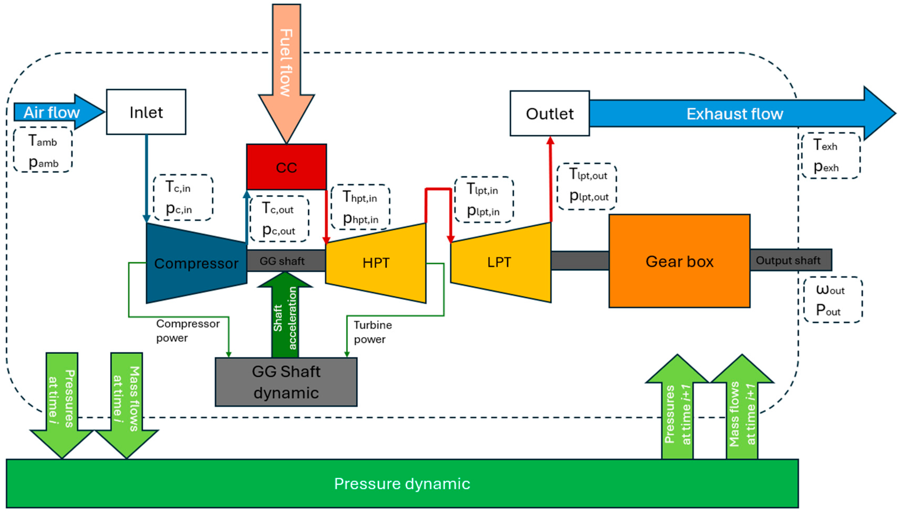
2.4. Numerical Model

The Simulink numerical model developed within this work is dynamic, modular, and parametric. The model was developed to correctly represent the system behavior in the typical engine’s operating range, combining look-up tables and physical considerations. The methodology used to develop the model has been extensively studied in the literature, proving accurate results with reduced computational cost [42,43,44,45,46,47].

The model was divided into 6 mains subsections: inlet, compressor, CC, HPT, LPT, and outlet. Each component was thermodynamically and physically connected, realizing instantaneous thermodynamic transformations upstream and downstream with the previous and following subsystems, respectively. As a result, the output flow characteristics of each component represent the input of the following section. To increase the accuracy of the model, especially during transients, iterative calculations were introduced to cover the pressure and mass flow rate dynamics in the engine. A schematic of the 0-D dynamic engine model is presented in Figure 3.

Based on physical considerations, the engine inlet was described as an adiabatic compression with a pressure loss only. The output of this component defined the compressor intake thermodynamic conditions, described by Equation (2):

$$\{\begin{array}{c}{T}_{tot,in}=T_{amb}\\ p_{tot,in}=p_{amb}\ast {\eta }_{inlet}\left({\dot{m}}_{c,in}\right)\end{array}$$

(2)

The subsystems representing the engine’s turbomachinery were modelled following isentropic laws (compression and expansions) per unit mass of fluid obtained in each machine and were corrected with the isentropic efficiency of each component (compressor, HPT, LPT) [48]. Equations (3) and (4) show how the compressor and turbines were described, where W_is is the isentropic specific work of the machine, W_re is the real specific work of the machine, c_p is the specific heat at constant pressure, R is the universal gas constant, T₁ is the temperature at the machine’s inlet, β is the compression ratio, γ is the heat capacity ratio, and η_is is the isentropic efficiency:

$$\{\begin{array}{c}{W}_{is,c}=-c_{p}R{T}_1\left({\beta }^{{\displaystyle \frac{\gamma -1}{\gamma }}}-1\right)\\ W_{re,c}={\eta }_{is,c}\left(\beta ,{\omega }_{norm},{\dot{m}}_{norm}\right)\ast W_{is,c}\end{array}$$

(3)

$$\{\begin{array}{c}{W}_{is,t}=c_{p}R{T}_1\left(1-{\displaystyle \frac{1}{{\beta }^{\frac{\gamma -1}{\gamma }}}}\right)\\ W_{re,t}={\eta }_{is,t}\left(\beta ,{\omega }_{norm},{\dot{m}}_{norm}\right)\ast W_{is,t}\end{array}$$

(4)

As can be seen in Equations (3) and (4), the value of η_is is a function of three normalized parameters: the compression/expansion ratio (β), the normalized rotational speed of the related shaft (ω_norm), and the normalized mass flow (${\dot{m}}_{norm}$). As is well known, since these parameters are physically linked, if two of these inputs are defined then the third is uniquely determined, reducing the efficiency to a function of only two of the three variables.

In the presented model, the efficiencies of each turbomachinery were described using look-up tables (provided by the engine manufacturer and validated using experimental data) with normalized mass flow rates and normalized rotational speeds as inputs. Although the values of c_p and γ are functions of the chemical composition, temperature, and pressure of the fluid, during this study, constant values for c_p and γ were considered based on the average temperature and pressure across each turbomachinery. Finally, an energy enthalpy balance has been used to obtain the total temperature (as the sum of static and dynamic temperatures) of the output flow for each subsystem.

The CC was modelled to produce an ideal (100% of fuel burned, and instantaneous chemical reactions) combustion process. The CC subsystem receives as input both air and fuel mass flows, as well as their thermodynamic characteristics. Then, the characteristics of the exhaust gases for both Jet A-1and hydrogen were obtained via the CEA-Run database. Finally, the model integrated two additional subsystems that feature the dynamic behavior of the GG shaft and the pressure dynamics inside each component. The dynamics of the GG have been modelled with a simple dynamic power balance (power generated by the HPT and power consumption of the compressor). Such a relationship is described by Equation (5), where ω is the rotational speed of the shaft, J is the rotational inertia of the shaft, P_T is the power produced by the turbine, P_C is the power consumption of the compressor, and P_E is the power losses of the GG system. As can be noticed, $P_E$ can also be represented as a decrease in the turbine power output through a dedicated efficiency term (${\eta }_m$).

$${\displaystyle \frac{d\omega }{dt}}={\displaystyle \frac{1}{J\omega }}\left(P_T-P_C-P_E\right)={\displaystyle \frac{1}{J\omega }}\left(P_T\ast {\eta }_m-P_C\right)$$

(5)

The pressure dynamics were mathematically described through a recursive implementation of the inter-component volume method aimed at calculating the values of pressure and mass flow in each section of the engine at each time step. The pressure variation was defined as defined in Equation (6), where V stands for the volume of the specific component and ${\dot{m}}_{in}$, ${\dot{m}}_{out}$ are the inlet and outlet mass flows of the subsystem, respectively. The calculation is iterated to reach convergence between the target pressure and mass flow rates that describe the different engine conditions generated by variations in the fuel flow rate.

$$\Delta p={{\displaystyle \int }}_{t_0}^{t_1}{\displaystyle \frac{\gamma RT}{V}}\left({\dot{m}}_{in}-{\dot{m}}_{out}\right)dt$$

(6)

The final step in the model design was focused on calibrating the turbomachinery performance maps provided by the manufacturer. In the literature, the extrapolation and validation of performance maps for different turbomachines, i.e., compressors and turbines, have been extensively studied [49,50,51,52]. Among others, the most effective solution is to adapt an existing performance map developed for an equivalent turbomachine using experimental data. In our study, we adapted the performance maps provided by the manufacturer with the experimental data obtained during a testing campaign.

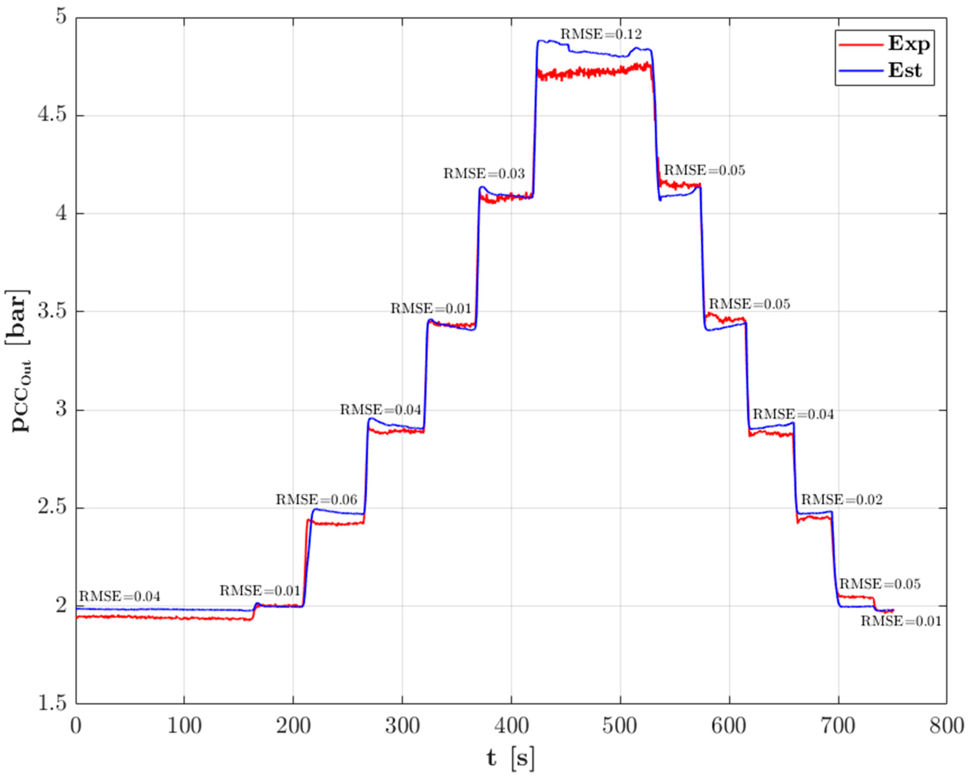
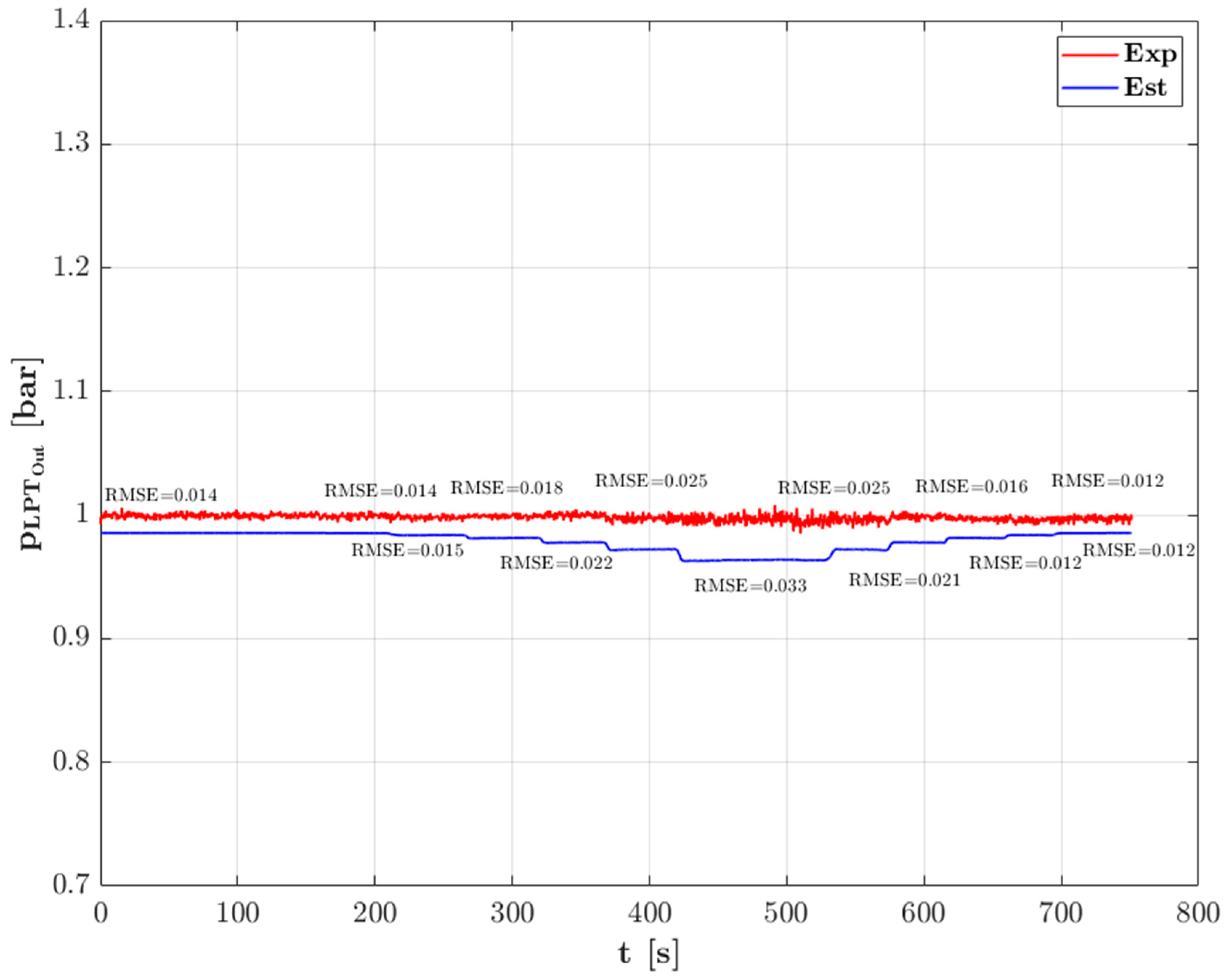
2.5. Thermocouple Dynamic

The 0-D dynamic model estimates the temperature of the air or exhaust gas flow within the engine, but such values are not completely representative of the temperature measured through a standard thermocouple due to the different thermal inertia of the sensor. With the aim of obtaining comparable results, the temperature of the hot junction in the thermocouple was estimated by using the 0-D equation of heat balance over the sensor body, as shown in Equation (7), where $k_{g-b}$ is the convective heat flux coefficient of the sensor body, $S_b$ is the sensor surface, $C_b$ is the heat capacity of the sensor, σ is the Boltzmann constant, ε is the emissivity, $T_b$, $T_g$ and $T_w$ are the temperature of the sensor body, the estimated temperature of the gas, and the temperature of the wall, respectively.

$${\displaystyle \frac{d{T}_b}{dt}}={\displaystyle \frac{k_{g-b}\ast S_b}{C_b}}\left(T_g-T_b\right)+{\displaystyle \frac{\sigma \ast \epsilon \ast S_b}{C_b}}\left(T_w^4-T_b^4\right)$$

(7)

Coupled with a simple heat balance applied to the wall (the irradiation term was neglected because of its small amplitude) as represented by Equation (8), where $k_{g-w}$ is the convective heat flux coefficient of the wall, $S_w$ is the wall surface, $C_w$ is the heat capacity of the wall, the sensor dynamic was recreated and compared to the experimental values.

$${\displaystyle \frac{d{T}_w}{dt}}={\displaystyle \frac{k_{g-w}\ast S_w}{C_w}}\left(T_g-T_w\right)$$

(8)

Similar approaches have already been validated in the literature [53]. Most of the parameters used to tune the equations have been obtained from the literature and are presented in

Table 3. List of parameters used in the thermocouple dynamic model [54,55].

${\mathit{k}}_{\mathit{g}-\mathit{b}}$ [W*m−2*C]	${\mathit{k}}_{\mathit{g}-\mathit{w}}$ [W*m−2*C]	$\mathit{\sigma }$ [W*m−2*K−4]	$\mathit{\epsilon }$ [-]	${\mathit{r}}_{\mathit{b}}$ [mm]	${\mathit{h}}_{\mathit{b}}$ [mm]	${\mathit{\rho }}_{\mathit{b}}$ [g/cm3]	${\mathit{c}}_{\mathit{b}}$ [J*g−1*C−1]
500	500	5.67 × 10−8	0.7	3.25	10.00	8.60	0.50

.

3. Results and Discussion

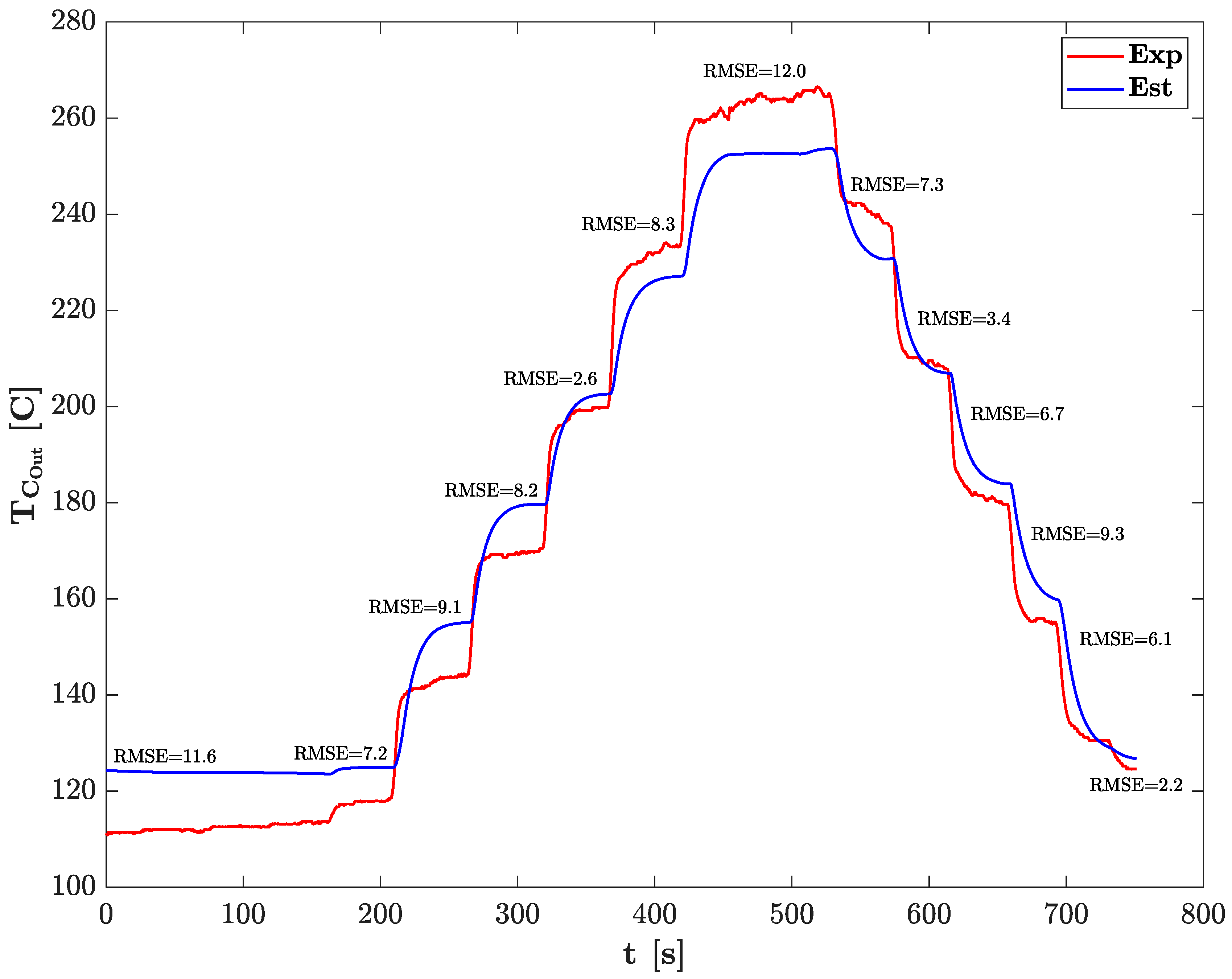
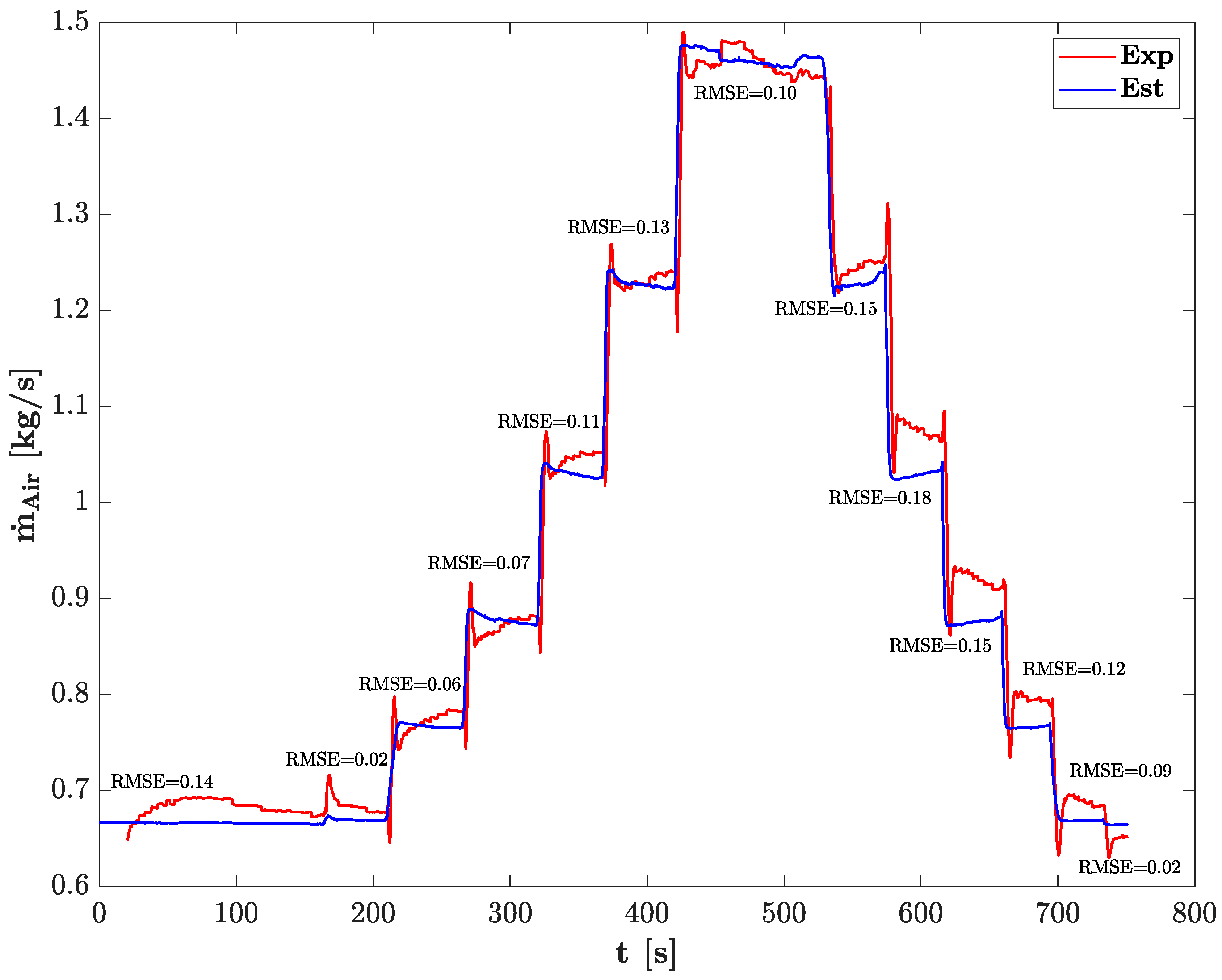
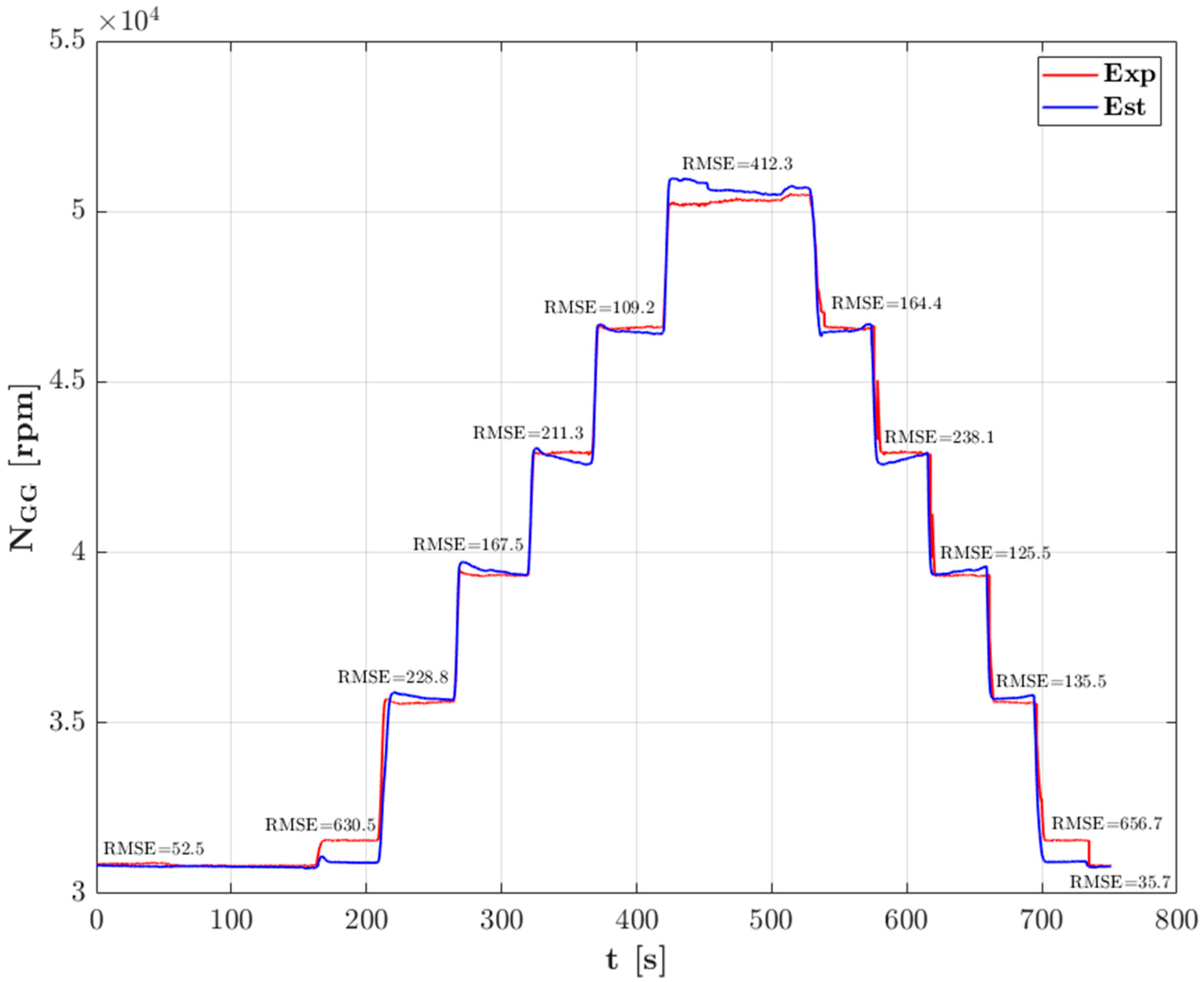
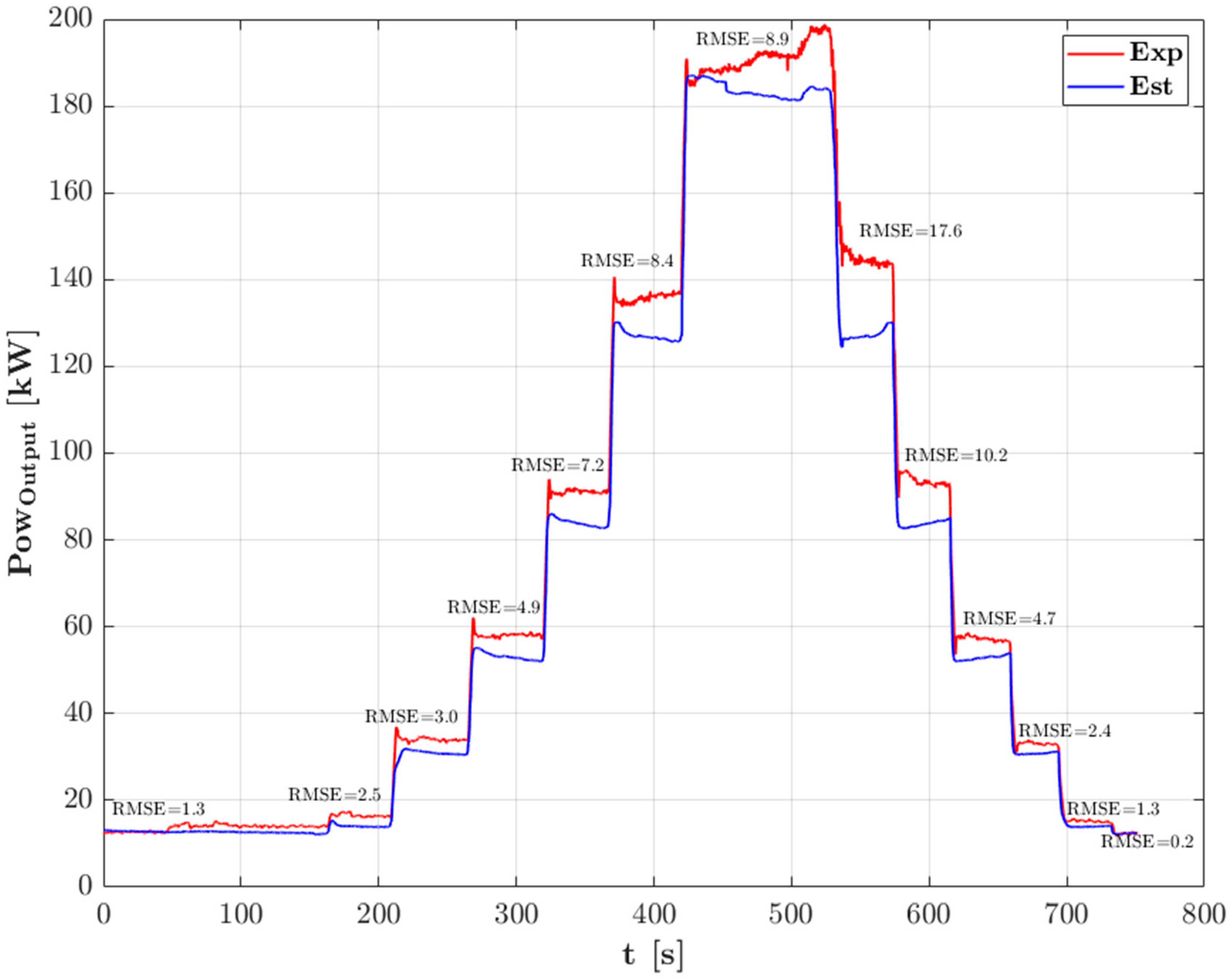
3.1. Model Validation

The 0-D dynamic model has been validated by comparing the model outputs with experimental data in a set of engine operating points using kerosene Jet A-1. During the testing activity, due to the engine characteristics, the operating point was controlled only by changing the throttle position, while the other engine parameters were mechanically and hydraulically controlled via the engine auxiliaries accordingly.

The load profile, expressed by the throttle level, used for the model validation is shown in Figure 4.

The process starts with a warm-up phase at idle conditions (up to 160 s), followed by a phase of ascending throttle (from 160 s to 520 s) and a symmetrical descending throttle phase (from 520 s to 750 s). The changes in the throttle input are instantaneous steps of finite dimension: in particular, five steps for both the ascending and descending phases from the idle condition to the maximum load. The inputs provided to the model are the air ambient conditions, the fuel mass flow rate corresponding to the throttle input, and the rotational speed of the brake, and consequently the output shaft.

Even though only a limited number of sensors could be placed on the engine, which does not cover the entirety of the characteristics obtained from the model, the quantities measured during the test include pressure and temperature levels at different sections of the engine and performance parameters. For the temperature, K-type thermocouples with ±2.2 °C accuracy were used for measurement. The pressure measurements were performed with a piezoresistive sensor with ±0.1% accuracy. The speed of the shaft was measured with a phonic wheel, with one tooth connected via a gear train to the GGS. The signal of the phonic wheel was collected by a variable reluctance sensor and preprocessed with a squaring circuit. The torque was measured with a single rotor Eddy Current Brake Dynamometer with an accuracy of ±0. 5% of the full scale, corresponding to ±1.287 kW. Finally, the air to fuel ratio, and indirectly the air mass flow, was measured via la lambda probe with an accuracy of ±0.002%.

Table 4. List of sensors mounted on the engine.

	External Conditions	Compressor Outlet	GG Shaft	CC Outlet	HPT Outlet	LPT Outlet	Brake
Thermodynamic parameters	p, T	p, T	-	p	p, T	p	-
Other parameters	-	-	RPM	-	-	λ	Poutput

shows the list of parameters that were experimentally measured during the testing campaign.

As depicted in Figure 5, the pressure estimation at the compressor outlet consistently keeps the RMSE below 0.20 bar stationaries.

Figure 5 shows that the maximum error of the model is located during the phase of maximum load, where the model underestimates the pressure provided by the compressor. Figure 6 shows the trend of the pressure level after the combustion chamber. The shape of the curve is very similar to the one presented in Figure 5 and shows very similar levels of error. This result was expected since the CC is a passive component, meaning that its effect on the pressure levels can be modelled with high accuracy.

As a further validation of the model’s accuracy in describing the engine pressure evolution, Figure 7 and Figure 8 show the trends of the HPT outlet pressure and engine outlet pressure, demonstrating good agreement with the experimental data. Figure 7 shows that the accuracy of the model does not present a substantial decrease throughout the different sections of the engine. The pressure at the exit of the HPT shows an inverted trend compared to the pressure at the exit of the compressor. The overestimation of both the compression and expansion ratios during the maximum load phase could be caused by a shifting of the stable condition of the turbo-group towards a condition with higher rotational speed. Finally, Figure 8 shows that the model slightly underestimates the pressure level at the exit of the engine (RMSE < 0.1 bar).

As shown in Figure 5, Figure 6, Figure 7 and Figure 8, the 0-D engine model outputs show overall high accuracy in describing the pressure within the engine, with RMSE not exceeding 0.2 bar. The occurrence of errors is mostly related to the relatively limited precision and quantity of data available to generate the efficiency maps of the turbomachines, with the maximum inaccuracy occurring during the maximum load phase, when the equilibrium of the machines is shifted towards higher speeds.

Figure 9 and Figure 10 show the evolution of the temperatures in the different sections of the engine. As can be seen, the temperature evolution in the main engine subsystems is characterized by the same behavior observed in the pressure, displaying the expected trends.

Looking at the temperature in the engine components, the magnitude of the percentage errors is always higher compared to the pressure levels, up to an RMSE of 50 K, in stationary conditions at the maximum load. The difference between experimental data and the numerical results obtained from the model is more marked after the combustion chamber. This observation suggests that the CEA has a limited capability to replicate the real combustion process taking place in the engine, but that it can correctly represent its trend. It is also important to note that the model underestimates the temperatures at maximum load at both the compressor and combustion chamber outlets. The analysis of the temperatures also shows a significant difference between the two phases of the test (distance between the ascending and descending sections of the test due to the thermal inertia of the system) during the experimental activity. This difference is related to the long-period thermal dynamics of the engine body and to the limited accuracy of the efficiency maps of the turbomachines when the engine is operated near the boundaries of its operating range (minimum and maximum load). The higher relevance in the results has been assigned to the data in the second half of the experimental test because it is considered closer to thermal equilibrium. To improve the accuracy of the 0-D engine model, the pressure dynamics should be coupled with the thermal analysis of the system, including both the thermal dynamics of the flow and the heat exchange with the environment. This solution would drastically increase the complexity and the computational cost of the model with little benefit in the model output compared to the real physical behavior of the engine. However, since the purpose of this model is to obtain a performance evaluation under steady-state conditions (when the engine is close to thermal equilibrium), it is reasonable to consider the model representative of the engine behavior and physically reliable.

Given that this study is intended to provide a preliminary performance comparison between Jet A-1and hydrogen, the accuracy of the results in terms of power was considered as more relevant.

In addition to the thermodynamic characteristics of the flow, the air mass flow inside the engine, the rotational speed of the GG shaft, and the power obtained at the output shaft were analyzed. Figure 11 shows the trend of the air mass flow rate that enters the engine. Both the model output and the experimental data are shown with an RMSE lower than 0.2 kg/s.

Comparing the experimental and simulated GG shaft speeds, as shown in Figure 12, the magnitude of the percentage error tends to zero in the first half of the test (from 2 to 525 s), where the load increases. In the second half of the test (from 525 to 753 s), the error remains practically unchanged. The largest differences occur in the first step over the idle condition (from 161 to 208 s), where the model slightly underestimates the rotational speed of the shaft compared to real values, and in the return to the idle at the end of the test (from 700 to 732 s), where the model similarly underestimates the rotational speed of the shaft. The overestimation of rotational speed generated relevant differences in the thermodynamic characteristics of the flow only in the phase of maximum load, where the second highest RMSE can be observed, while in the first step of load after idle the error is negligible. This result shows the sensitivity of the model to the accuracy of the turbomachines’ performance maps, showing significant variations in the air flow thermodynamic conditions as a result of small variations in the shape of the performance maps.

Finally, Figure 13 shows the power obtained at the output shaft of the engine. The model globally tends to underestimate the power, with an average RMSE during steady-state conditions on the order of magnitude of 10 kW, due to the sum of previous inaccuracies of the model (especially those related to the thermal behavior).

Considering the results presented in this section, the 0-D dynamic engine model developed in this study has demonstrated that it provides sufficiently accurate estimations of the engine parameters and performance, with errors fluctuating around 10% of the measured data in steady-state conditions.

The in-depth analysis of the results identified the lack of a numerical representation for heat rejection and heat exchange with the environment coupled with the limited accuracy of the efficiency maps available, as the main sources of discrepancies between the model output and the experimental data. Nonetheless, the physical response of the model is well-aligned with the experimental behavior of the engine and the performance of other models presented in the literature, making the model a valid candidate for further analysis.

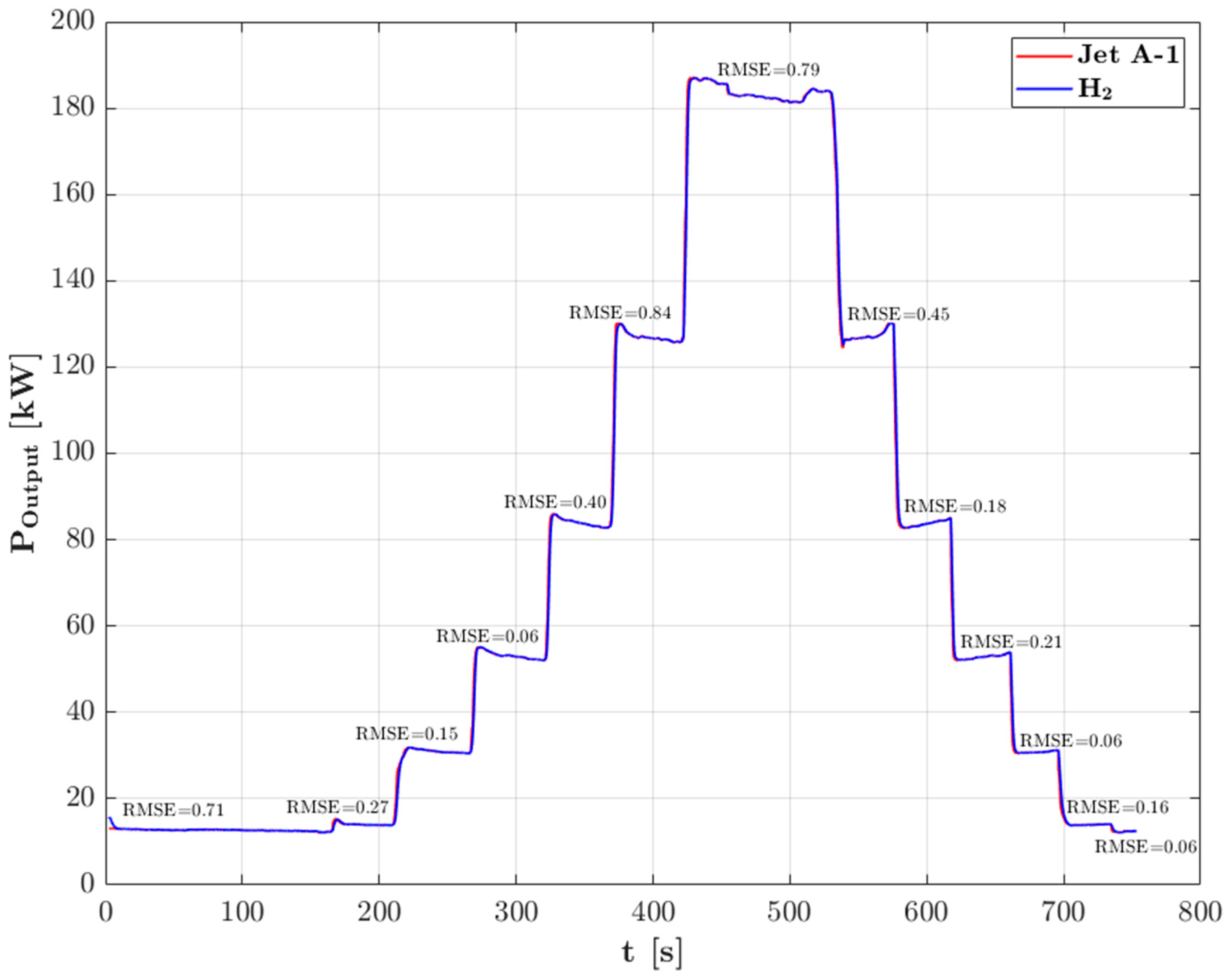
3.2. Performance Comparison between Kerosene Jet A-1 and Hydrogen

The second objective of this study was to investigate the performance of the Allison 250 C-18 operating with gaseous hydrogen.

The assumptions made to perform the comparison are summarized below:

• Constant engine power output.
• No hardware modifications.
• Similar environmental conditions.

The comparison was performed with the power output profile obtained from the simulation during the validation of the model presented in Figure 13. This profile was chosen over the measured power output to provide a fair comparison between two different simulations (kerosene Jet A-1 and hydrogen) obtained under similar assumptions. For this reason, to provide the same engine power output using hydrogen, a PID (Proportional Integral Derivative) controller was considered to dynamically adapt the hydrogen mass flow rate. Keeping the engine power output constant provides a relevant insight toward the performance of hydrogen in real scenarios. It is worth mentioning that the absence of hardware modifications and consistent ambient conditions gives further consistency to the comparison, as it does not introduce modifications to the structure of the model that could invalidate the analysis. The only modification in the model was focused on the combustion chamber, in which the simplified combustion model (based on the CEA-Run database) was modified to operate with hydrogen.

Figure 14 shows the comparison between the engine power output when running on kerosene Jet A-1 and on hydrogen. The two outputs are extremely close (RMSE < 1%). The results shown in Figure 14 also confirm that, in terms of the quality of the combustion process with hydrogen, if similar conditions in the combustion chamber are created using conventional geometry and components (injection system and combustion chamber), stable working conditions can be achieved. Table 4 summarizes the maximum and average variations between hydrogen and Jet A-1 for the fundamental engine parameters running the 0-D dynamic model. To quantify the difference in the main engine parameters operating on H₂ and Jet A-1 over the whole test, the Maximum Percentage Difference (MPD)—expressed by Equation (9), where $a_{H^2}$ and $a_{Jet A-1}$ represent the values of the generic engine parameters operating hydrogen and Jet A-1, respectively—and the Average Percentage Difference were both calculated.

$$Maximum Percentage Difference (\%)=max\left({\displaystyle \frac{a_{H^2}-a_{Jet A-1}}{a_{Jet A-1}}}\right)\ast 100$$

(9)

Both MPD and APD consider Jet A-1 as the reference fuel, leading to positive variations when using hydrogen.

The working conditions between the two simulations do not present relevant variations, but do highlight different engine behaviors when running on hydrogen. As is evident in

Table 5. Maximum (MPD) and Average (APD) percentage difference of the main engine parameters operating the 0-D dynamic engine model with hydrogen and Jet A-1.

	MPD (%)	APD (%)
Air mass flow (kg\s)	+8.0%	+2.3%
Total mass flow (kg\s)	+7.1%	+1.5%
GGS rotational speed (rpm)	+5.2%	+1.3%
β compressor (-)	+8.8%	+2.3%
β HPT (-)	+7.5%	+1.8%
β LPT (-)	−4.5%	−0.4%
Cp after the combustion (J\K*kg)	+3.5%	+1.6%

, the GG behavior is characterized by a higher rotational speed of the shaft, mass flow rate, and compression ratio (compressor) in all working conditions. The increases in air mass flow rate and compression ratio are directly related to the higher rotational speed at which the group finds a dynamic equilibrium based on the turbine and compressor power balance (stable condition). The LPT and the corresponding shaft, on the other hand, show a small decrease in expansion ratio at the same rotational speed (fixed value from the reduction gear input of 2.8940 × 10⁴ rpm).

A crucial aspect of running hydrogen in turbine engines is related to the exhaust flow characteristics (temperature and specific heat of the gas mixture), which have an impact on engine performance. Since the hydrogen LHV is three times higher compared to Jet A-1, an average 64% reduction in the fuel mass flow rate was found between the two simulations. Figure 15 shows the comparison between hydrogen and kerosene Jet A-1 mass flow rates. Despite this result constituting a great advantage of hydrogen over Jet A-1 in aeronautical applications, where weight reduction is one of the main design criteria, the increase in weight derived by the hydrogen storage systems required on-board compensates for this advantage. The simulation output clearly shows that when running on hydrogen, the temperature at the end of the combustion is lower by an average of 20° C compared to Jet A-1 due to the higher dilution of the injected fuel when running on hydrogen (the same engine components were considered during this study). This aspect is strictly connected to the quantity and composition of the exhaust gases. The amount of exhaust gases is slightly smaller but has a higher concentration of water vapor and nitrogen when running on hydrogen. The water vapor is characterized by a higher specific heat compared to the carbon-based end-gas of conventional fuels, leading to cooler exhaust flow at equal energy released from the combustion process. Figure 16 shows the comparison between hydrogen and kerosene Jet A-1 exhaust temperatures.

To provide a fair comparison between the performance of the two fuels, the kerosene Equivalent Brake Specific Fuel Consumption when running on hydrogen was calculated and compared to the standard BSFC (calculated using kerosene as a fuel), both in terms of absolute values and the average percentage difference (APD) for each throttle level. The results of this comparison are shown in Figure 17, demonstrating an average reduction in fuel consumption of 1.1% when running on hydrogen. The decrease in specific fuel consumption tends to increase in magnitude moving toward the maximum load. The magnitude of the difference does not constitute a significant improvement of hydrogen compared to kerosene Jet A-1 for engineering applications. On the other hand, the similar performance displayed by hydrogen constitutes a valuable outcome, guaranteeing consistency in the engine performance of aeronautical propulsion systems against the backdrop of a conversion toward sustainability.

Moreover, from the analysis shown in Figure 18, which illustrates the thermal efficiency of the engine and its average difference (AD) at each throttle level, it can be seen that the efficiency at maximum load is increased by 0.23% when running on hydrogen (blue line) compared to kerosene Jet A-1 (red line), while the remaining engine conditions show very similar performance, with a slightly improved efficiency of 0.12% on average. This result further confirms the assumption proposed during the analysis shown in Figure 14, Figure 17 and Figure 18, in which a fairly constant performance—in terms of engine power output, BSFC, and thermal efficiency—can be obtained by the 0-D engine model using kerosene Jet A-1 and hydrogen.

4. Conclusions

This paper presents a preliminary numerical investigation of the performance of an aeronautical turbine engine operated with gaseous hydrogen. For this purpose, a 0-D dynamic engine model was developed and validated using kerosene Jet A-1, testing the real engine in a test cell. Several data sets have been acquired, with the aim of collecting enough data to describe the engine behavior over its whole engine operating range. Through the assumptions and the modelling procedure followed in this study, the numerical engine model has shown accurate physical and thermodynamic outputs, close to the real engine behavior, in all the tested conditions.

After the validation of the model, the tool was used to perform a preliminary comparison of the engine operating on hydrogen, collecting information both in terms of performance and the physical and thermodynamic behavior of the engine, and showing a result of very similar behavior.

Combining the outcome of this activity with a pros and cons analysis related to the adoption of hydrogen in air mobility, the following conclusions can be drawn:

• Due to its much higher LHV, hydrogen reaches the same energy as Jet A-1 with a reduced mass flow rate. Hydrogen revealed a reduction of approximately 64% in fuel flow rate to obtain the same power output as Jet A-1. This condition implies that the fraction of aircraft weight dedicated to fuel could be greatly reduced from an energy standpoint. However, this positive effect cannot be fully exploited with the current generation of hydrogen tanks, which are much heavier compared to traditional aeronautical tanks.
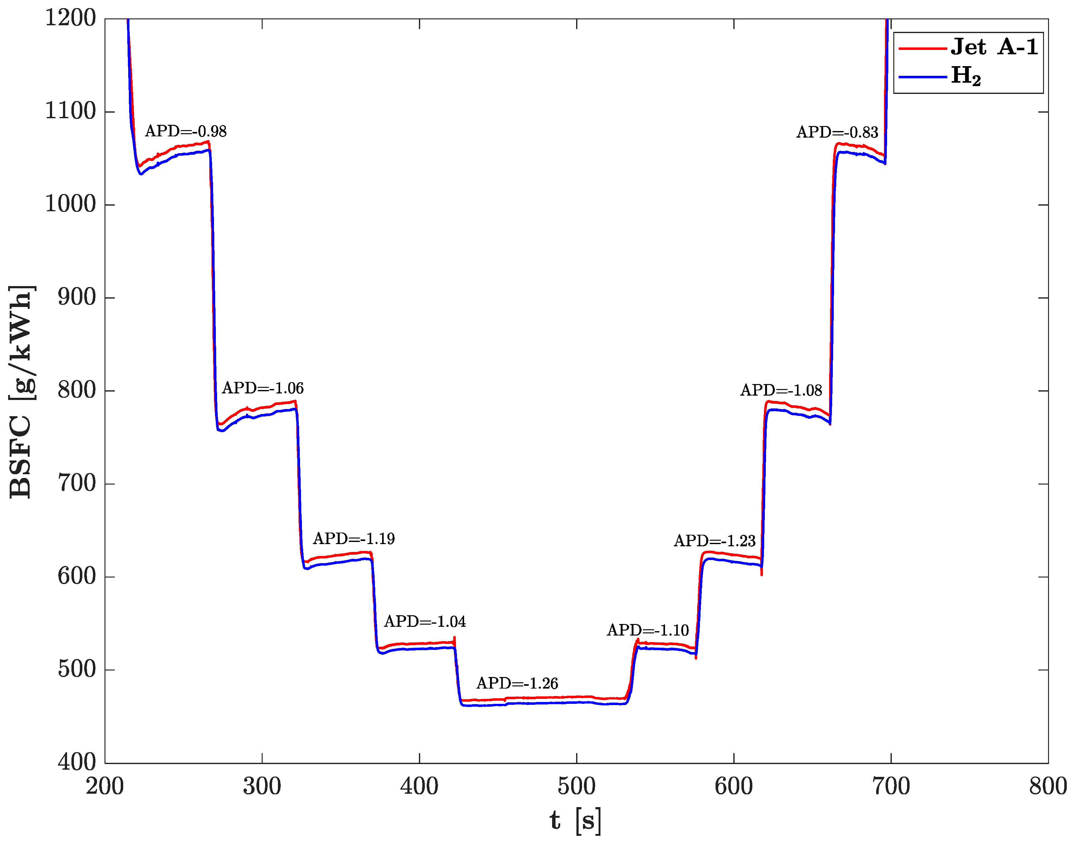
• The similar specific fuel consumption indicates that conventional aircraft could perform similar missions with the same amount of energy stored in the fuel tank system. At ambient conditions, hydrogen is characterized by a mass density five orders of magnitude lower than kerosene, with an LHV only three times higher, requiring pressurized and/or cryogenic tanks to be stored in acceptable volumes. The estimated mass of these tanks compared to Jet A-1 tanks varies significantly in different previous studies, from a maximum increase of 66%. Nonetheless, all studies agree on an increase in the volume of the tank of at least five times.
• Since gaseous hydrogen is CO₂-free, the quantity of CO₂ present in the combustion of hydrogen is limited to the percentage of CO₂ initially present in the air. This result represents the main advantage of hydrogen over conventional fossil fuels in terms of reducing the environmental impact of air traffic.
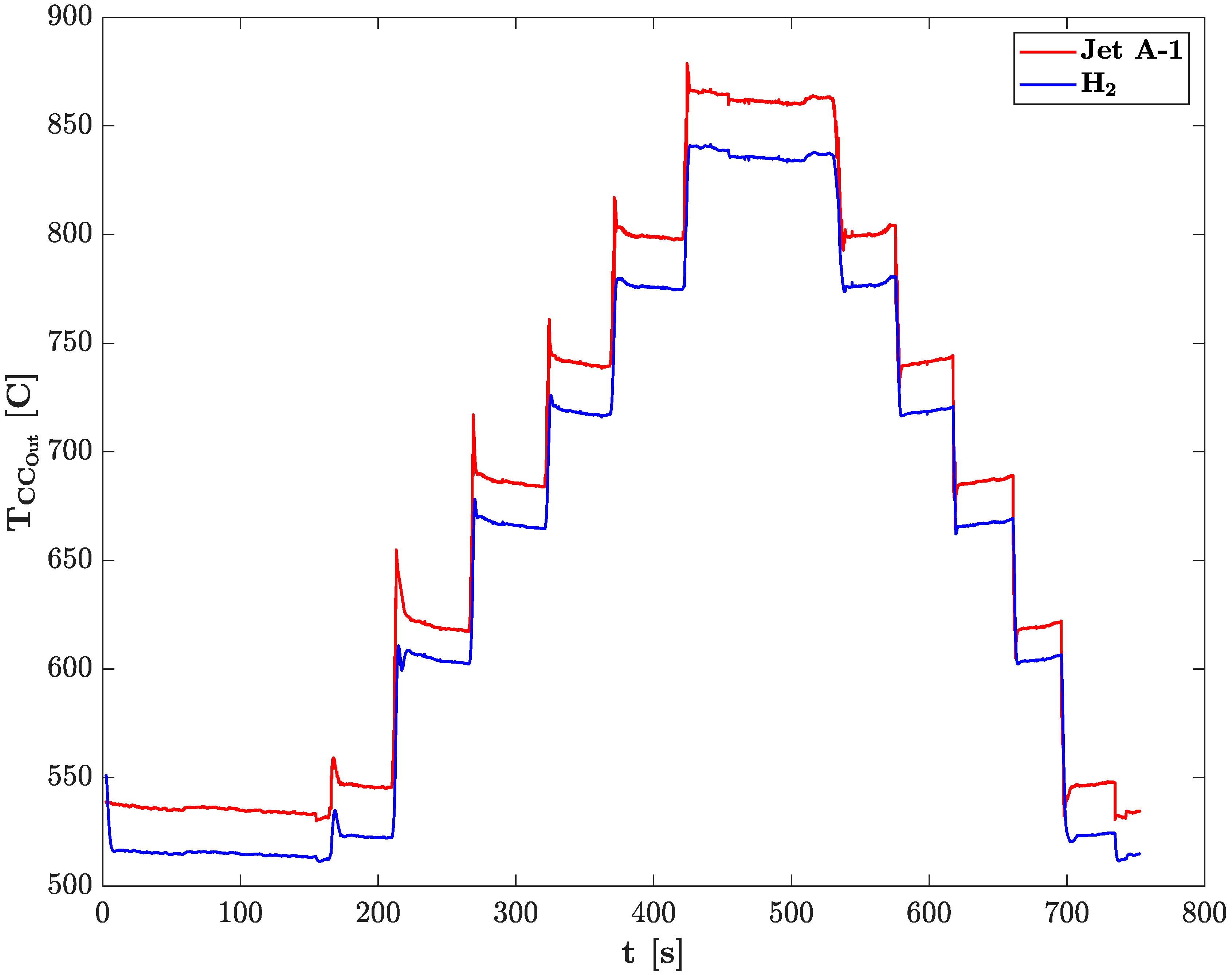
• Running on hydrogen, the temperature of the engine sections after the CC is lower. At the outlet of the combustion chamber, an average decrease of 2.2% in temperature was observed. Taking into account the thermal and structural limitations of today’s materials, hydrogen would be able to produce more power while reaching the same temperature at the exit of the combustion chamber, either by introducing more fuel or reducing the air intake.
• The decrease in temperature at the inlet of the turbines is partially compensated by the increase in specific heat of the gas (mixture running on hydrogen). The increase in the specific heat (approximately 1.6%) may be related to the higher presence of water vapor in the exhaust flow.
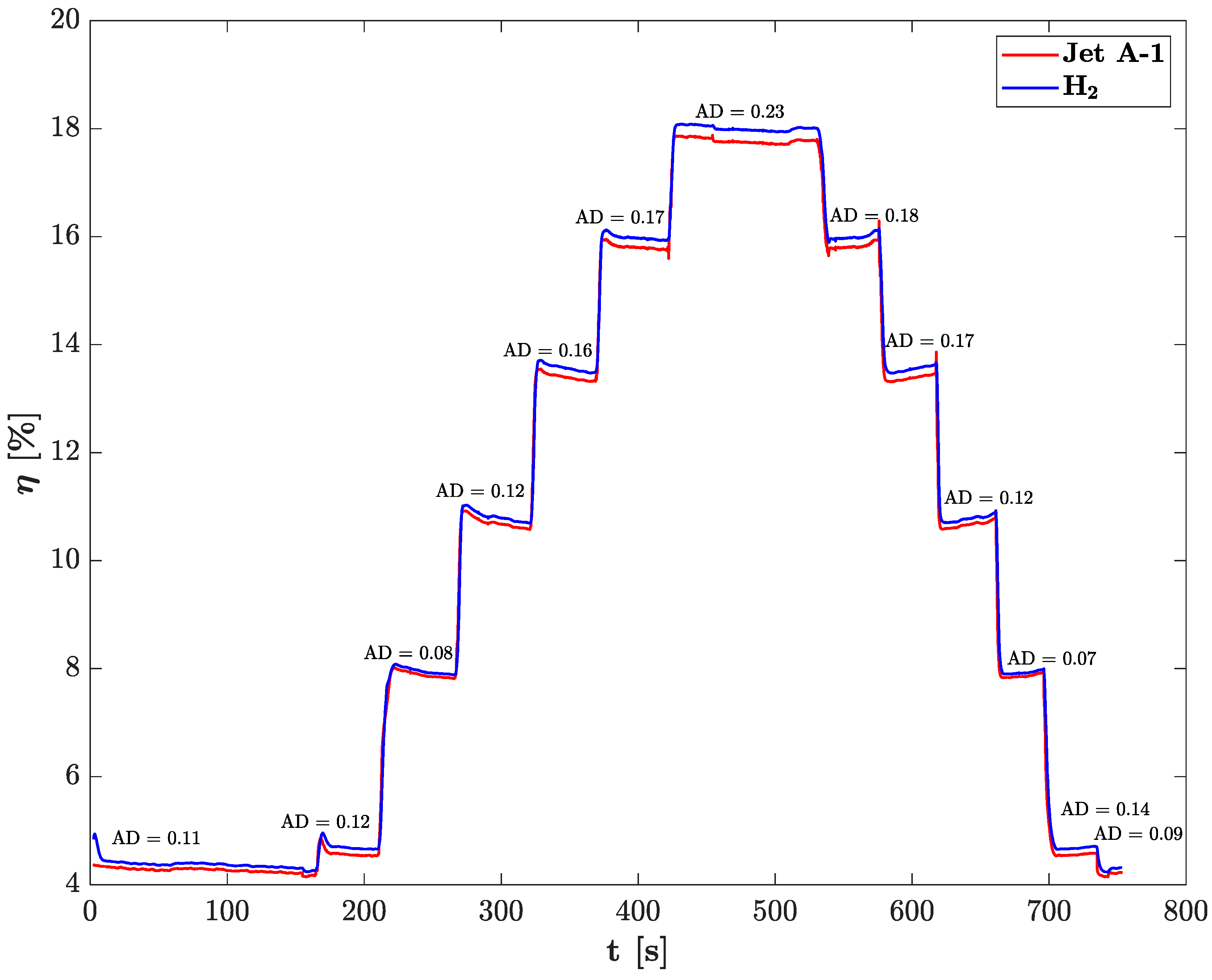
• Running on hydrogen, the dynamic power balance of the GG has been shifted toward different engine conditions, characterized by higher rotational speed, increased air mass flow rate, and an increased compression ratio. Only the LPT has shown lower efficiency at the new operating points (no efficiency variations were recorded for either the compressor or the HPT).

Further activities are currently ongoing to convert the engine to operate on hydrogen, coupling CFD 3D simulation of the hydrogen flow through the conventional combustion chamber and hardware modifications of the engine to operate on hydrogen. Combining the present study with future research and detailed investigations of new components aimed at handling hydrogen (tanks, delivery systems, injectors, valves), it will be possible to further extend the research on hydrogen solutions for achieving a greener and more sustainable aviation.

References

1. Climate Change 2022, Mitigation of Climate Change.pdf. Available online: https://www.ipcc.ch/report/ar6/wg3/downloads/report/IPCC_AR6_WGIII_SummaryForPolicymakers.pdf (accessed on 23 February 2024).
2. Climate Change and Sustainable Transport UNECE. Available online: https://unece.org/transport/climate-change-and-sustainable-transport (accessed on 11 March 2024).
3. Transforming Our World: The 2030 Agenda for Sustainable Development|Department of Economic and Social Affairs. Available online: https://sdgs.un.org/2030agenda (accessed on 18 March 2024).
4. Sustainable Development Goals—European Commission. Available online: https://international-partnerships.ec.europa.eu/policies/sustainable-development-goals_en (accessed on 11 March 2024).
5. Communication from the Commission to the European Parliament, the European Council, the Council, the European Economic and Social Committee and the Committee of the Regions. The European Green Deal. 2019. Available online: https://eur-lex.europa.eu/legal-content/EN/TXT/?uri=COM%3A2019%3A640%3AFIN (accessed on 11 March 2024).
6. Transport—Energy System. Available online: https://www.iea.org/energy-system/transport (accessed on 18 March 2024).
7. Martin, J.; Neumann, A.; Ødegård, A. Renewable hydrogen and synthetic fuels versus fossil fuels for trucking, shipping and aviation: A holistic cost model. Renew. Sustain. Energy Rev. 2023, 186, 113637. [Google Scholar] [CrossRef]
8. Ebrie, A.S.; Kim, Y.J. Investigating Market Diffusion of Electric Vehicles with Experimental Design of Agent-Based Modeling Simulation. Systems 2022, 10, 28. [Google Scholar] [CrossRef]
9. Su-ungkavatin, P.; Tiruta-Barna, L.; Hamelin, L. Biofuels, electrofuels, electric or hydrogen?: A review of current and emerging sustainable aviation systems. Prog. Energy Combust. Sci. 2023, 96, 101073. [Google Scholar] [CrossRef]
10. Tajuddin, M.H.B. The Comparison Study between Aviation Jet A-1 And Super Bio-Jet Fuel (Jatropha Based) Usages on Allison 250 Mockup Gas Turbine Engine. 2013. Available online: https://ir.unikl.edu.my/xmlui/handle/123456789/3912 (accessed on 6 December 2023).
11. Almena, A.; Siu, R.; Chong, K.; Thornley, P.; Röder, M. Reducing the environmental impact of international aviation through sustainable aviation fuel with integrated carbon capture and storage. Energy Convers. Manag. 2024, 303, 118186. [Google Scholar] [CrossRef]
12. Corchero, G.; Montañés, J.L. An approach to the use of hydrogen for commercial aircraft engines. Proc. Inst. Mech. Eng. Part G J. Aerosp. Eng. 2005, 219, 35–44. [Google Scholar] [CrossRef]
13. Brewer, G.D. Hydrogen Aircraft Technology; Routledge: London, UK, 2017; ISBN 978-1-351-43979-4. [Google Scholar]
14. Adler, E.J.; Martins, J.R.R.A. Hydrogen-powered aircraft: Fundamental concepts, key technologies, and environmental impacts. Prog. Aerosp. Sci. 2023, 141, 100922. [Google Scholar] [CrossRef]
15. Tiwari, S.; Pekris, M.J.; Doherty, J.J. A review of liquid hydrogen aircraft and propulsion technologies. Int. J. Hydrogen Energy 2024, 57, 1174–1196. [Google Scholar] [CrossRef]
16. Degirmenci, H.; Uludag, A.; Ekici, S.; Karakoc, T.H. Challenges, prospects and potential future orientation of hydrogen aviation and the airport hydrogen supply network: A state-of-art review. Prog. Aerosp. Sci. 2023, 141, 100923. [Google Scholar] [CrossRef]
17. Prewitz, M.; Schwärzer, J.; Bardenhagen, A. Potential analysis of hydrogen storage systems in aircraft design. Int. J. Hydrogen Energy 2023, 48, 25538–25548. [Google Scholar] [CrossRef]
18. Gimenez, F.R.; Mady, C.E.K.; Henriques, I.B. Assessment of different more-electric and hybrid-electric configurations for long-range multi-engine aircraft. J. Clean. Prod. 2023, 392, 136171. [Google Scholar] [CrossRef]
19. Chiara Massaro, M.; Pramotton, S.; Marocco, P.; Monteverde, A.H.A.; Santarelli, M. Optimal design of a hydrogen-powered fuel cell system for aircraft applications. Energy Convers. Manag. 2024, 306, 118266. [Google Scholar] [CrossRef]
20. Nicolay, S.; Karpuk, S.; Liu, Y.; Elham, A. Conceptual design and optimization of a general aviation aircraft with fuel cells and hydrogen. Int. J. Hydrogen Energy 2021, 46, 32676–32694. [Google Scholar] [CrossRef]
21. Massaro, M.C.; Biga, R.; Kolisnichenko, A.; Marocco, P.; Monteverde, A.H.A.; Santarelli, M. Potential and technical challenges of on-board hydrogen storage technologies coupled with fuel cell systems for aircraft electrification. J. Power Sources 2023, 555, 232397. [Google Scholar] [CrossRef]
22. Ringuedé, A.; Hubert, S.; Atwi, L.; Lair, V. Prospects of hydrogen and its derivative as energy vector for electricity production at high temperature: Fuel cells and electrolysers. Curr. Opin. Electrochem. 2023, 42, 101401. [Google Scholar] [CrossRef]
23. Haglind, F.; Singh, R. Design of Aero Gas Turbines Using Hydrogen. J. Eng. Gas Turbines Power 2006, 128, 754–764. [Google Scholar] [CrossRef]
24. Chiesa, P.; Lozza, G.; Mazzocchi, L. Using Hydrogen as Gas Turbine Fuel. J. Eng. Gas Turbines Power-Trans. ASME 2005, 127, 73–80. [Google Scholar] [CrossRef]
25. Adam, A.; He, W.; Fan, Y.; Han, D. Investigation of flow characteristics and mixing of liquid hydrogen within a premixing swirl tube for the turbine engine combustor. Int. J. Hydrogen Energy 2024, 49, 367–383. [Google Scholar] [CrossRef]
26. Funke, H.H.-W.; Keinz, J.; Kusterer, K.; Ayed, A.H.; Kazari, M.; Kitajima, J.; Horikawa, A.; Okada, K. Development and Testing of a Low NOx Micromix Combustion Chamber for Industrial Gas Turbines. Int. J. Gas Turbine Propuls. Power Syst. 2017, 9, 27–36. [Google Scholar] [CrossRef]
27. Haj Ayed, A.; Kusterer, K.; Funke, H.H.-W.; Keinz, J.; Striegan, C.; Bohn, D. Experimental and numerical investigations of the dry-low-NOx hydrogen micromix combustion chamber of an industrial gas turbine. Propuls. Power Res. 2015, 4, 123–131. [Google Scholar] [CrossRef]
28. Aircraft Certification|EASA. Available online: https://www.easa.europa.eu/en/domains/aircraft-products/aircraft-certification (accessed on 24 March 2024).
29. Babahammou, H.R.; Merabet, A.; Miles, A. Technical modelling and simulation of integrating hydrogen from solar energy into a gas turbine power plant to reduce emissions. Int. J. Hydrogen Energy 2024, 59, 343–353. [Google Scholar] [CrossRef]
30. Balli, O.; Ozbek, E.; Ekici, S.; Midilli, A.; Hikmet Karakoc, T. Thermodynamic comparison of TF33 turbofan engine fueled by hydrogen in benchmark with kerosene. Fuel 2021, 306, 121686. [Google Scholar] [CrossRef]
31. Wang, X.; He, A.; Hu, Z. Transient Modeling and Performance Analysis of Hydrogen-Fueled Aero Engines. Processes 2023, 11, 423. [Google Scholar] [CrossRef]
32. Paoli, M.D.; Ponti, D.I.F. Validazione Preliminare del Modello Dinamico di un Turboalbero Aeronautico. Master’s Thesis, Università di Bologna, Bologna, Italy, 2014. [Google Scholar]
33. M250 Turboshaft. Available online: https://www.rolls-royce.com/products-and-services/civil-aerospace/helicopters/m250-turboshaft.aspx (accessed on 25 March 2024).
34. The M250—A Model Engine|Rolls-Royce. Available online: https://www.rolls-royce.com/media/our-stories/discover/2018/the-m250-a-model-engine.aspx (accessed on 27 March 2024).
35. Type Certificate Data Sheets (TCDS)|EASA. Available online: https://www.easa.europa.eu/en/document-library/type-certificates (accessed on 17 September 2024).
36. 250-C18-Operation-Maintenance-Manual.pdf. Available online: https://pscorp.ph/wp-content/uploads/2019/06/250-C18-Operation-Maintenance-Manual.pdf (accessed on 25 March 2024).
37. Chemical and Physical Information. In Toxicological Profile for JP-5, JP-8, and JET A Fuels; Agency for Toxic Substances and Disease Registry (US): Atlanta, GA, USA, 2017. Available online: https://www.ncbi.nlm.nih.gov/books/NBK592027/ (accessed on 30 March 2024).
38. Table 1. ASTM Fuel Specification Test Results for Jet A-1. Available online: https://www.researchgate.net/figure/ASTM-FUEL-SPECIFICATION-TEST-RESULTS-FOR-JET-A-1_tbl1_267501767 (accessed on 30 March 2024).
39. The Energy Density of Hydrogen: A Unique Property. Demaco Cryogenics. 2024. Available online: https://demaco-cryogenics.com/blog/energy-density-of-hydrogen (accessed on 30 March 2024).
40. McBride—Sanford Gordon and Associates Cleveland, Ohio.pdf. Available online: https://ntrs.nasa.gov/api/citations/19950013764/downloads/19950013764.pdf (accessed on 30 March 2024).
41. NASA-RP-1311-2.pdf. Available online: https://shepherd.caltech.edu/EDL/PublicResources/sdt/refs/NASA-RP-1311-2.pdf (accessed on 30 March 2024).
42. Camporeale, S.M.; Fortunato, B.; Mastrovito, M. A Modular Code for Real Time Dynamic Simulation of Gas Turbines in Simulink. J. Eng. Gas Turbines Power 2002, 128, 506–517. [Google Scholar] [CrossRef]
43. Kim, S.-K.; Pilidis, P.; Yin, J. Gas Turbine Dynamic Simulation Using Simulink®; SAE Technical Paper 2000-01–3647; SAE International: Warrendale, PA, USA, 2000. [Google Scholar] [CrossRef]
44. Eastbourn, S.; Roberts, R. Modeling and Simulation of a Dynamic Turbofan Engine Using Simulink. In Proceedings of the 47th AIAA/ASME/SAE/ASEE Joint Propulsion Conference & Exhibit, San Diego, CA, USA, 31 July–3 August 2011; American Institute of Aeronautics and Astronautics: Reston, VA, USA, 2023. [Google Scholar] [CrossRef]
45. Asgari, H.; Venturini, M.; Chen, X.; Sainudiin, R. Modeling and Simulation of the Transient Behavior of an Industrial Power Plant Gas Turbine. J. Eng. Gas Turbines Power 2014, 136, 061601. [Google Scholar] [CrossRef]
46. Roberts, R.A.; Eastbourn, S.M. Modeling Techniques for a Computational Efficient Dynamic Turbofan Engine Model. Int. J. Aerosp. Eng. 2014, 2014, e283479. [Google Scholar] [CrossRef]
47. Hashmi, M.B.; Lemma, T.A.; Ahsan, S.; Rahman, S. Transient Behavior in Variable Geometry Industrial Gas Turbines: A Comprehensive Overview of Pertinent Modeling Techniques. Entropy 2021, 23, 250. [Google Scholar] [CrossRef] [PubMed]
48. Dixon, S.L. Fluid Mechanics and Thermodynamics of Turbomachinery, 4th ed.; in SI/metric units; Butterworth-Heinemann: Boston, MA, USA, 1998; ISBN 978-0-7506-7059-3. [Google Scholar]
49. Venturini, M. Development and Experimental Validation of a Compressor Dynamic Model. J. Turbomach. 2004, 127, 599–608. [Google Scholar] [CrossRef]
50. Tsoutsanis, E.; Meskin, N.; Benammar, M.; Khorasani, K. A component map tuning method for performance prediction and diagnostics of gas turbine compressors. Appl. Energy 2014, 135, 572–585. [Google Scholar] [CrossRef]
51. Aldi, N.; Morini, M.; Pinelli, M.; Spina, P.R.; Suman, A. Cross Validation of Multistage Compressor Map Generation by Means of Computational Fluid Dynamics and Stage-Stacking Techniques. In Volume 3B: Oil and Gas Applications; Organic Rankine Cycle Power Systems; Supercritical CO2 Power Cycles; Wind Energy; American Society of Mechanical Engineers: Düsseldorf, Germany, 2014; p. V03BT25A009. [Google Scholar] [CrossRef]
52. GmbH, G. GasTurb—Smooth C/T. Available online: https://www.gasturb.com/software/smooth-c-t.html (accessed on 17 September 2024).
53. Liu, B.; Huang, Q.; Wang, P. Influence of surrounding gas temperature on thermocouple measurement. Case Stud. Therm. Eng. 2020, 19, 100627. [Google Scholar] [CrossRef]
54. Manjhi, S.K.; Kumar, R. Performance assessment of K-type, E-type and J-type coaxial thermocouples on the solar light beam for short duration transient measurements. Measurement 2019, 146, 343–355. [Google Scholar] [CrossRef]
55. Demsis, A.; Verma, B.; Prabhu, S.V.; Agrawal, A. Heat transfer coefficient of gas flowing in a circular tube under rarefied condition. Int. J. Therm. Sci. 2010, 49, 1994–1999. [Google Scholar] [CrossRef]
Figure 1. Allison 250 C-18 graphical representation [36].
Aerospace 11 00816 g001
Figure 2. Allison 250 C-18 flow path and component detail [36].
Aerospace 11 00816 g002
Figure 3. Schematic of the 0-D dynamic engine model.
Aerospace 11 00816 g003
Figure 4. Load profile during the experimental campaign.
Aerospace 11 00816 g004
Figure 5. Measured (red line) and estimated (blue line) pressures at the compressor outlet and RMSE for each load step.
Aerospace 11 00816 g005
Figure 6. Measured (red line) and estimated (blue line) pressure at the CC outlet and RMSE for each load step.
Aerospace 11 00816 g006
Figure 7. Measured (red line) and estimated (blue line) pressure at the HPT outlet and RMSE for each load step.
Aerospace 11 00816 g007
Figure 8. Measured (red line) and estimated (blue line) pressure at the LPT outlet and RMSE for each load step.
Aerospace 11 00816 g008
Figure 9. Measured (red line) and estimated (blue line) temperature at the compressor outlet and RMSE for each load step.
Aerospace 11 00816 g009
Figure 10. Measured (red line) and estimated (blue line) temperature at the HPT outlet and RMSE for each load step.
Aerospace 11 00816 g010
Figure 11. Measured (red line) and estimated (blue line) Air mass flow rate at the engine’s inlet and RMSE for each load step.
Aerospace 11 00816 g011
Figure 12. Measured (red line) and estimated (blue line) rotational speed of the GG shaft and RMSE for each load step.
Aerospace 11 00816 g012
Figure 13. Measured (red line) and estimated (blue line) engine power output and RMSE for each load step.
Aerospace 11 00816 g013
Figure 14. Engine power output comparison using kerosene Jet A-1 (red line) and hydrogen (blue line) in the 0-D dynamic engine model and RMSE for each load step.
Aerospace 11 00816 g014
Figure 15. Fuel mass flow rate comparison using kerosene Jet A-1(red line) and hydrogen (blue line) in the 0-D dynamic engine model.
Aerospace 11 00816 g015
Figure 16. Combustion chamber outlet temperature comparison and average difference (AD) using kerosene Jet A-1 (red line) and hydrogen (blue line) in the 0-D dynamic engine model for each tested throttle level.
Aerospace 11 00816 g016
Figure 17. BSFC comparison using kerosene Jet A-1 (red line) and hydrogen (blue line) in the 0-D dynamic engine model and ADP ranging from 50% to 90% load (throttle position).
Aerospace 11 00816 g017
Figure 18. Thermal efficiency of the engine and average difference (AD) using kerosene Jet A-1 (red line) and hydrogen (blue line) in the 0-D dynamic engine model for each tested throttle level.
Aerospace 11 00816 g018