Abstract
Flow through complex thermodynamic machinery is intricate, incorporating turbulence, compressibility effects, combustion, and solid–fluid interactions, posing a challenge to classical physics. For example, it is not currently possible to simulate a three-dimensional full-field gas flow through the propulsion of an aircraft. In this study, a new approach is presented for predicting the real-time fluid properties of complex flow. This perspective is obtained from deep learning, but it is significant in that the physical context is embedded within the deep learning architecture. Cases of excessive working states are analyzed to validate the effectiveness of the given architecture, and the results align with the experimental data. This study introduces a new and appealing method for predicting real-time fluid properties using complex thermomechanical systems.
1. Introduction
Complex thermodynamic machinery has intricate flow characteristics. Among these, turbulence is typically observed in engineering [1,2,3]. Turbulence is regarded as one of the challenging problems in classical physics [4], characterized by complex flow parameters, substantial temporal fluctuations, and marked features of non-uniformity and irregularity. Considerable effort has been devoted to the analysis of complex flow, particularly the internal flow through complicated thermodynamic machinery [5,6]. Unfortunately, it has not been possible thus far to simulate a three-dimensional full-field gas flow through the propulsion of an aircraft owing to the complexity of its structure and working process. Therefore, real-time prediction of the flow parameter in complex thermodynamic machinery is currently difficult. Furthermore, monitoring the operation of thermodynamic machinery in real time, such as the safety monitoring of aircraft engine operations, is challenging. Moreover, the lack of dual redundancy monitoring, which relies on real-time prediction, poses significant hidden dangers to the safe operation of thermal machinery.
Deep learning is a class of computing systems designed to learn to perform tasks directly from raw data without hard-coding task-specific knowledge, which has received increasing attention in recent years [7,8,9]. This system has gained popularity due to its versatility and revolutionary success in various domains [10,11,12]. In addition, deep learning has raised optimism for solving complex flow problems in engineering [13,14]. However, deep learning processes are generally not interpretable. It is critical to know the reasons behind a decision made by a deep learning system to avoid hidden dangers in various domains, such as aerospace, nuclear engineering, and civil aviation [15]. This is particularly important for complex mechanical systems, such as aircraft engines, that operate in harsh environments and require high levels of safety. Therefore, the explained deep learning model has become an urgent topic of exploration [16,17].
Underlying the above comments is the notion that deep learning may provide a new perspective for investigating flow through thermodynamic machinery, even though it is a complex phenomenon related to mathematics, physics, and engineering. A method for discovering the fundamental links from complex flow architectures to deep learning networks is an appealing prospect. The direct incorporation of differentiable physical equations as network layers in a neural network is an interesting method for establishing the fundamental links [18,19]. For instance, PINO, or Physics-Informed Neural Operator, is an approach that models differential operators through neural operators and is particularly tailored for addressing partial differential equations (PDEs) in physics [20,21,22]. Introducing algebraic constraints into the loss function of a deep learning network to train a deep learning model [23,24,25] is also a method for establishing the fundamental links.
Nevertheless, it is not easy to use differential equations describing the complete working process in many mechanical engineering applications, such as the intricate flow through an aircraft engine. This affects the development of the method for establishing the fundamental links between complex thermodynamic machinery and deep learning networks. In this study, an alternative approach called physics-embedded deep learning is presented for linking physical and network architectures to facilitate the real-time prediction of the fluid properties of complex flows for engineering. This approach refines the overall mechanical system into a combination of individual component models, coupling those models using physical architecture. It emphasizes the coupling relationship between the components and the overall system, avoiding limitations introduced by strict adherence to physical equations, while efficiently predicting the parameters of complex flow inside the complete machinery system. Several challenging cases across a wide range of working states and important scientific and engineering problems of aircraft engines are investigated.
2. Complex Flow in the Propulsion of Aircraft
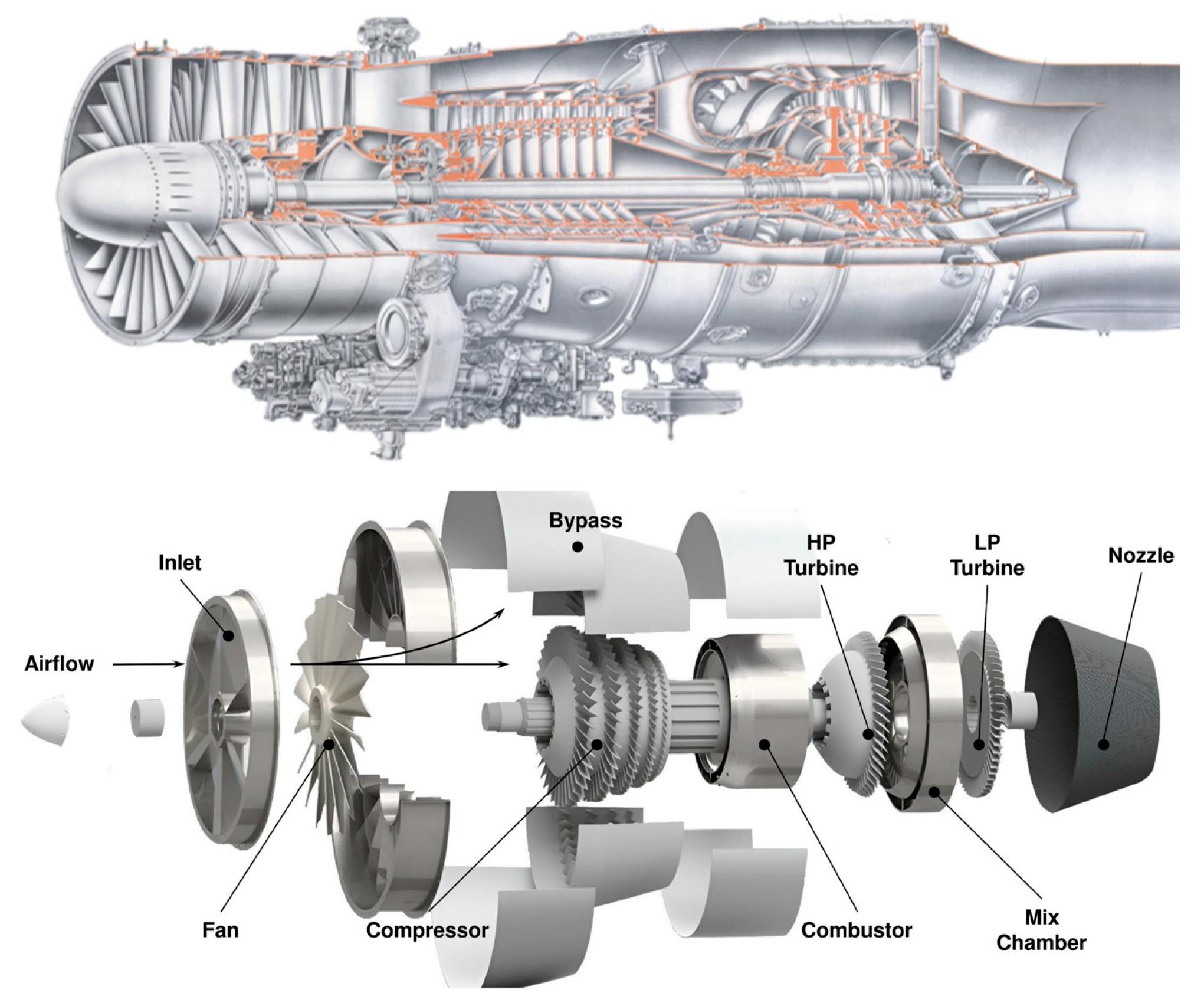
A turbofan is a type of airbreathing jet engine widely used in aircraft propulsion [26]. A typical modern turbofan produces thrust to power aircraft by ingesting ambient air, compressing the air, undergoing combustion, and expanding the hot gas through thrust-producing exhaust nozzles, as shown in the schematic cross-section in Figure 1. As shown in the figure, a low-pressure compressor, usually known as a fan, compresses air into a bypass duct, and its inner portion supercharges the core compressor. A fan is often an integral part of a multi-stage core low-pressure compressor. The bypass airflow either passes through a separate ‘cold nozzle’ or mixes with hot gases from the low-pressure turbine exhaust before expanding through the ‘mixed-flow nozzle’.
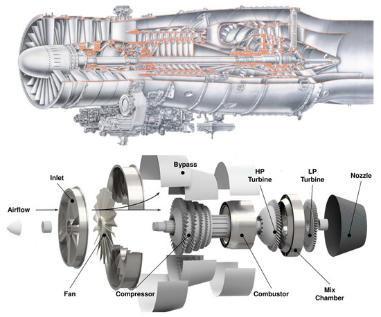
Figure 1.
Structural diagram of a low-bypass turbofan engine.
The design of a turbofan typically begins with a study of the complete engine using a relatively simple aerothermodynamic ‘cycle’ analysis. The operating characteristics of turbofan components, such as the fan, compressor, and turbine, are represented in this study by performance maps that are based on experimental test data [27,28]. The design of individual engine components is further refined, simulated, and experimentally tested in isolation by component design teams as the process progresses. These results are then used to calibrate the component performance maps and improve the cycle analysis of the complete engine. The process continues with the refined component designs until the component and engine performance goals are met. The design trade-offs between engine performance and component performance still deserve in-depth study [29]. Component design teams rely on advanced numerical techniques to understand component operations and achieve optimal performance. Although advanced numerical simulations of isolated components may yield detailed performance data at unique component operating points, they do not account for the systematic interactions between the engine components. The overall engine performance is dependent on the components working together efficiently over a range of demanding operating conditions. However, several components are sensitive to interactions with adjoining components [30]. Consequently, it is important to consider the engine as a system of components that influence each other, and not simply as isolated components. However, a detailed simulation of a complete turbofan engine requires considerable computational capacity. A three-dimensional, viscous, and unsteady aerodynamic simulation of a gas turbine engine requires approximately 1012 floating-point operations per second, with a multidisciplinary analysis two to three times that value [31]. Today, this computing power is only available on a few expensive supercomputers with a large number of processors.
As outlined above, traditional methods are not applicable for real-time fluid property prediction. Thus, new methods are required to meet the increasing need for engineering and fundamental research. Fortunately, recent advances in deep learning have created new possibilities for real-time fluid property prediction in the field of complex flow, particularly for the treatment of the internal flow of complex thermodynamic machinery.
Deep learning is the name used for ‘stacked neural networks’ that are composed of several layers [32]. The layers are composed of nodes. A node is simply a place where computation occurs and is loosely patterned on a neuron in the human brain that fires when it encounters sufficient stimuli. A node combines the input from the data with a set of coefficients or weights that either amplify or dampen that input, thereby assigning significance to inputs regarding the task that the algorithm is trying to learn. Deep learning networks are distinguished from the more commonplace single-hidden-layer neural networks by their depth; that is, the number of node layers that data must pass through in a multistep process of a scheduled task. Each layer of nodes in a deep learning network is trained on a distinct set of features based on the output of the previous layer. The further one advances into the neural net, the more the nodes can recognize complex features because they aggregate and recombine features from the previous layer. Underlying the above comments on deep learning is the fact that information in the nodes of a neural network is nonphysical and driven by training data. Although classical deep learning has advantages, such as savings in computational efficiency, it also has flaws concerning current engineering problems, such as issues with generalization and the need for large amounts of training data [33].
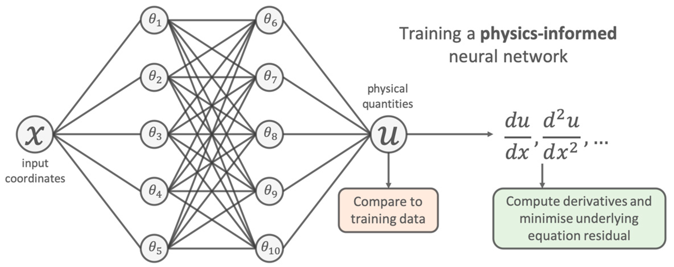
A more recent strategy involves combining physical principles and traditional algorithms with deep learning in a more nuanced manner to create more powerful models in the burgeoning field of scientific deep learning [34]. An effective way to create a hybrid model is to synergistically combine data-driven and model-based approaches [35]. Another approach that has received significant attention is the use of physics-informed neural networks that can be used to solve forward and inverse problems related to differential equations [36,37]. In this approach, a deep neural network is used to represent the solution of a differential equation that is trained using a loss function and directly penalizes the residual of the underlying equation, as shown in Figure 2.
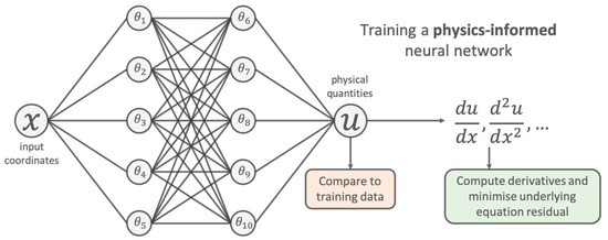
Figure 2.
Schematic of physics-informed neural network.
Physics-informed neural networks have multiple benefits in comparison with classical methods. For example, they provide approximate mesh-free solutions that have tractable analytical gradients and an elegant method of carrying out joint forward and inverse modeling [38]. Although popular and effective, this approach has significant limitations when compared with classical approaches, such as poor computational efficiency [39] and poorly understood theoretical convergence properties [40,41]. However, there are no differential equations describing the complete working process in many complex mechanical engineering applications, such as the complex flow in an aircraft engine considered in this study. This not only affects the development of such approaches but also makes the investigation of complex physical problems in engineering very challenging.
3. Physics-Embedded Deep Learning for Investigating Complex Flow in Turbofan Engines
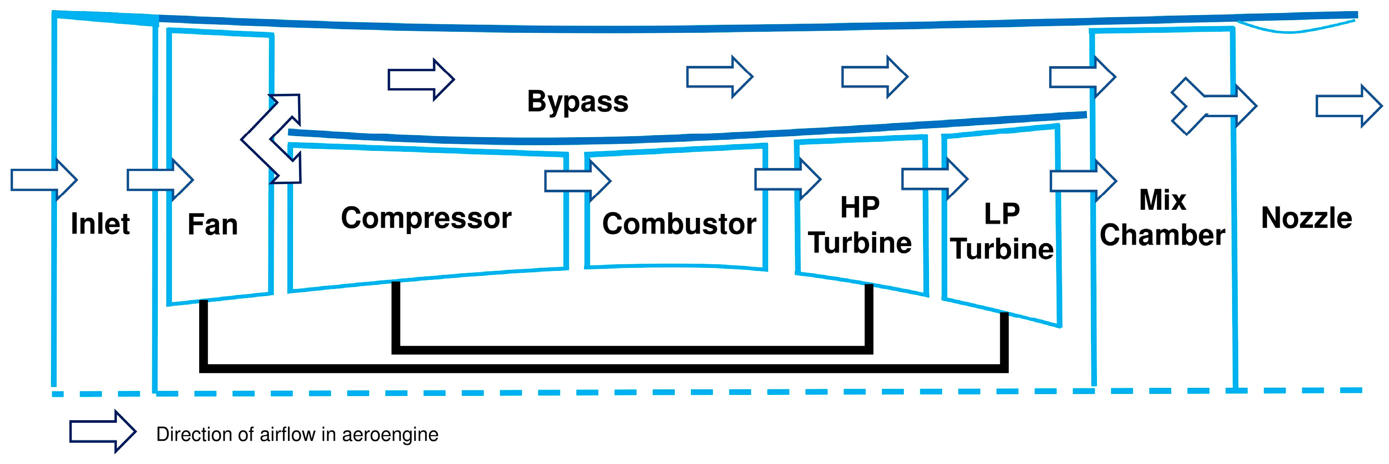
A new domain decomposition approach, called physics-embedded deep learning, is presented in this study for solving large, multi-scale physical problems related to complex mechanical engineering. As mentioned previously, a turbofan operates by ingesting ambient air through the inlet, compressing the air through the fan and compressor, undergoing combustion through the combustor, generating work through high- and low-pressure turbines to drive the fan and compressor, respectively, and expanding the hot gas through the nozzles. In particular, a fan, usually known as a low-pressure compressor, compresses air into a bypass duct as its inner portion supercharges the compressor. The bypass airflow is passed to a mixing chamber with low-pressure turbine exhaust gases before expanding through the nozzle. These various component systems work together according to certain physical laws during the operation of an aircraft engine, as shown in Figure 3. The main goal of physics-embedded deep learning is to address the coupling of the working process and mechanism described above, which is achieved using domain decomposition.
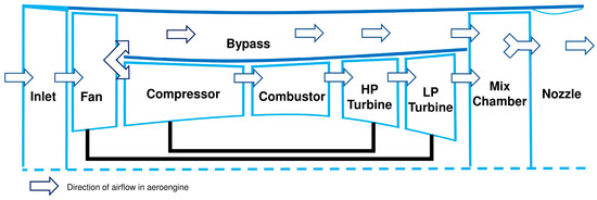
Figure 3.
Working process of a turbofan engine.
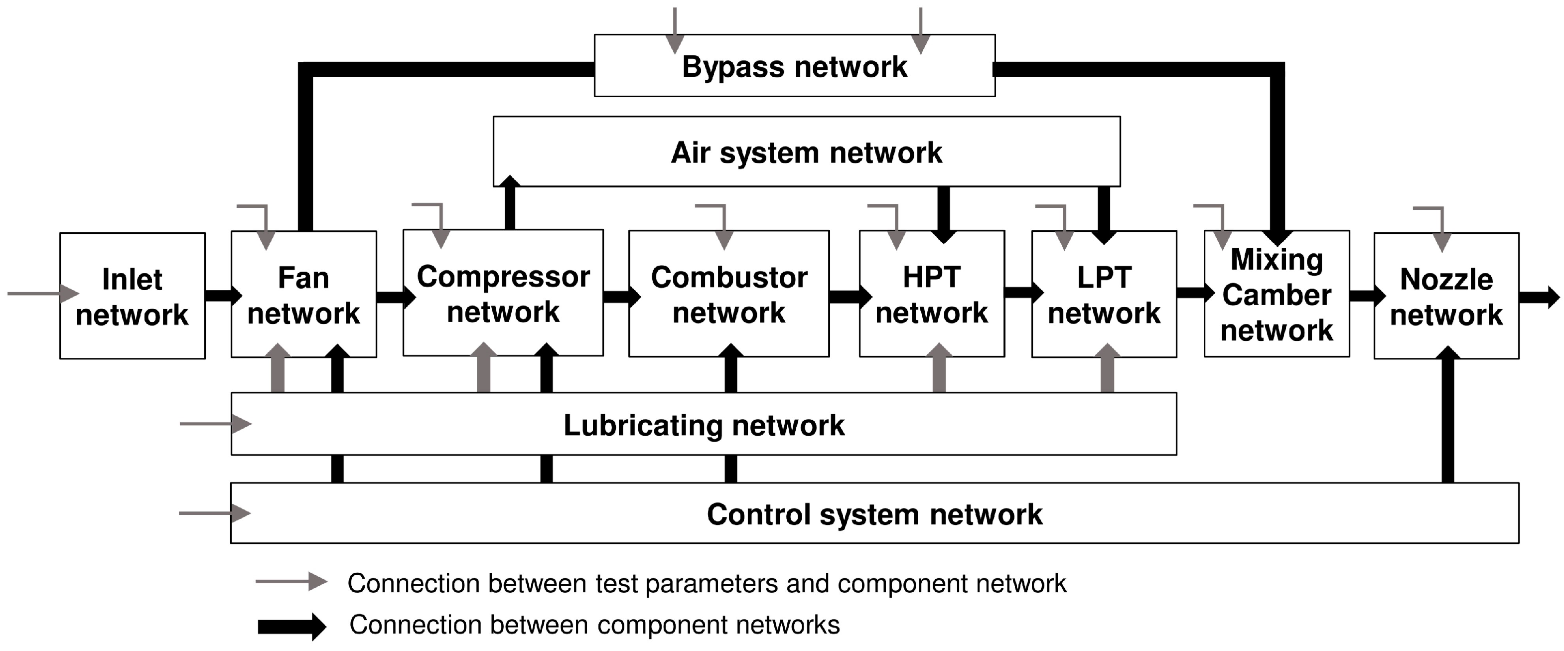
Engineers are expected to understand how these components work together. In contrast, researchers normally emphasize the discovery of physical laws. Therefore, components are transferred from physical to digital space matching to facilitate using an artificial intelligence network. Each independent learning network is used to represent the physical components, such as the inlet, fan, and compressor, as shown in Figure 4. In the physical space, air enters the fan and compressor components through the inlet; therefore, there is a data transmission relationship between the inlet, fan, and compressor networks in the digital space. The cooling air system in an aircraft engine includes a compressor bleed conduit extending from the compressor to the turbine blade cooling fluid supply that provides cooling fluid to at least one turbine blade. Therefore, an air system network was created in the digital space that transmitted data from the compressor network to the turbine network. The primary purpose of a lubrication system is to deliver oil to the internal engine components. These components are directly related to the fans, compressors, and high- and low-pressure turbines. Thus, the lubricating network inputs data into the fan, compressor, and high- and low-pressure turbine networks. Furthermore, the data link relationship of the control system network has a one-to-one correspondence with the physical aircraft engine. The test parameters are sent to their corresponding networks during the data training process. For example, the compressor speed is sent to the compressor network rather than to the fan network.
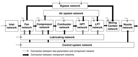
Figure 4.
Aircraft engine component matching in digital space.
The domain decomposition method involves dividing the entire computational domain into several subdomains, solving each subdomain, and finally coupling the solutions of subdomains through coordination strategies. In physics-embedded deep learning, the independent learning network used to represent the physical component is collectively referred to as a component network. Assuming a node within a component network is represented by , and a component network is represented by NN, the complex connections between nodes form a component network. The specific ways of connection between nodes are not discussed here (discussed in Section 4), and the structure of a component network is represented by NN(). The output of a component network is:
where H represents the output of a component network, i indicates the location of the component network, xi is the input parameters corresponding to the component/system i, and Hk represents the component network output that is unidirectionally linked to component network i. The equation reveals that the decoupling of the independent computational domain is determined by the relationship between the engine’s physical components. This relationship denotes a direct connection between a physical component of the engine and other physical components, leading to data transmission in the corresponding computational domain. Therefore, solving the entire computational domain is equivalent to learning the coupling relationships between all of the engine components:
Here g denotes engine components in the air system, s represents system or bypass, y(xi) signifies the output of the entire computational domain, xi refers to input parameters, and xg and xs, respectively, represent the inputs to the corresponding component networks, including input parameters and outputs from other component networks.
Representation learning involves the acquisition of effective features from data to enhance the representation and capture vital information. Deep learning serves as an approach to representation learning, as it views the hidden layers of neural networks as hierarchically learning representations of input data, succinctly expressed by:
Here i denotes input, NNi represents the input layer, and NNh represents the hidden layer in deep learning. Comparing Equations (2) and (3) reveals that in physics-embedded deep learning, the embedded physical knowledge restricts the number of parameters entering the component network. Different input parameters define the output representation of independent computational domains and mitigate the impact of irrelevant input parameters on independent computational domains. From the above equations, it is inferred that the solution of the independent component network is equivalent to the performance of the related physical components/systems, and the coupling between component networks is analogous to the co-working relationship in engine components. In the equivalent relationship, the operation of an aircraft engine conventionally represented by physical equations is directly substituted with network learning. The physics-embedded deep learning fundamentally avoids the human-made factors introduced by physical modeling, making it easier to characterize the operation of complex thermodynamic machinery. Therefore, physics-embedded deep learning explicitly articulates the hierarchical features of the data, facilitating the prediction of complex flow parameters on the engine component section.
4. Component Networks
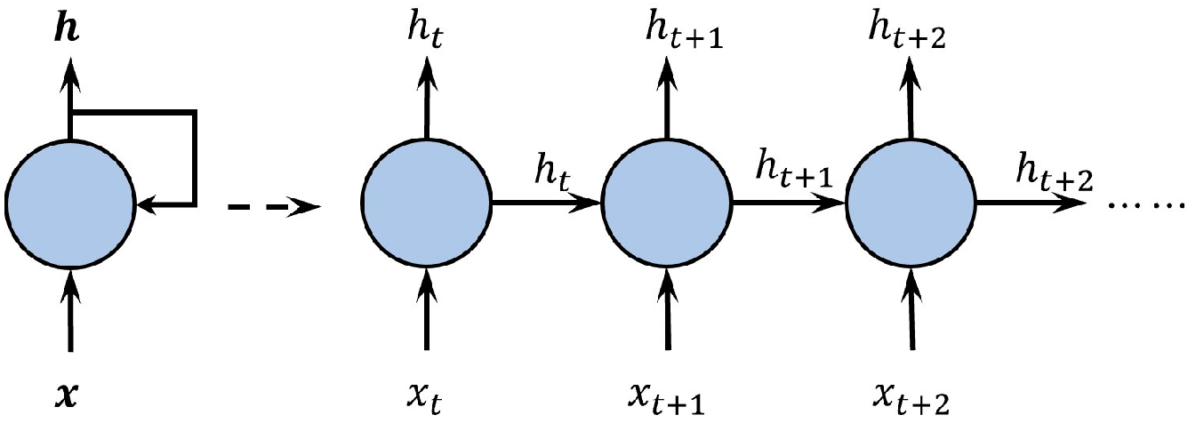
Component networks played a critical role in training the presented deep learning approach. In addition, the influences of the measurement parameter space and time series must be considered within networks. One alternative approach is to use a mature artificial intelligence network, such as a recurrent neural network (RNN) [42]. An RNN is a deep learning network that is ideal for sequential data because it uses iterative calculations that enable nodes to incorporate current inputs and past results. In an RNN, a structure composed of nodes participating in iterative calculations is called a cell. This is unlike conventional network architectures that process inputs as separate independent nodes. Cells at different iterative times are linked in a chain by unfolding the iterative calculation in sequential order. This represents the transfer of information in a time or space sequence, as shown in Figure 5. However, RNNs lose past information in deep sequential data owing to the vanishing gradient problem. A long short-term memory (LSTM) neural network was introduced to address this problem, which is a memory cell with three gate units that increase the flexibility of information processing [43].

Figure 5.
Schematic of unfolded RNN.
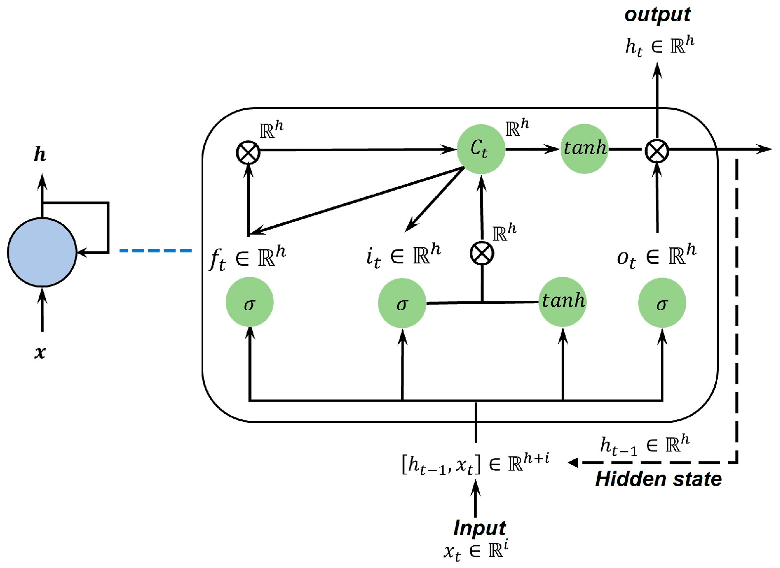
Compared with conventional RNNs, the processing of information flow in an LSTM cell is multi-threaded instead of single-threaded. The inner components of an LSTM cell are presented in Figure 6.
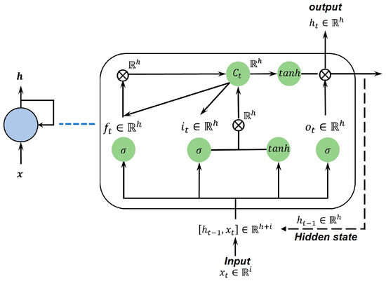
Figure 6.
The inner components of an LSTM cell.
At the t-th time, an LSTM cell receives an input vector xt, the hidden state is the same as the previous output of cell ht−1, and one output vector ht is produced. For a forward pass, a combined vector of the input x and hidden state ht−1 is fed into the cell. The vector is controlled by the input, forget, and output gate functions, which determine the amount of information that should be kept, forgotten, and outputted for the current state of the cell, respectively. These gate functions are respectively expressed as:
where denotes the sigmoid function, xt denotes the input data at time t in a sequence of length l, W denotes the weight matrix, and b denotes the bias vector. i, f, and o denote the elements associated with the input, forget, and output gates, respectively. ht−1 denotes the hidden state in which the values are the same as the output result from the previous calculation.
Subsequently, a candidate cell state at time t is calculated based on the input vector and hidden state. The cell state C at time t is updated by the cell state from the previous time and candidate cell. These values are also controlled by the input and forget gates. These calculations are expressed as:
Finally, the output of cell h at time t is computed, which is expressed as:
5. Results
5.1. Real-Time Prediction of the Exhaust Gas Temperature
The real-time prediction of the exhaust gas temperature (EGT) was considered as the first case study. The EGT is typically defined as the gas temperature at the exit of an aircraft engine and is considered a key parameter for optimizing fuel economy, diagnosis, and prognosis. The turbine blade temperature is a key indicator of the normal life consumption of a blade. However, direct sensor measurements for turbine modules are limited because of the extremely hot environment. Consequently, frequent malfunctions occur, leading to low reliability in temperature measurements. The EGT sensors located downstream from the highest-temperature sections provide a means to approximately infer the temperatures of the turbine blades/disks. These sensors are also considered the most vulnerable elements of the entire turbine engine instrumentation. Real-time and accurate EGT values are particularly vital for high-performance military turbofan engines, where the margin between hot-section operating conditions and material limitations is shrinking. Therefore, the real-time and accurate prediction of EGT holds significant value. Traditional fluid simulation methods encounter a huge challenge in the field of real-time flow parameter prediction in that the complex flow through an aircraft engine cannot be completely simulated in real time.
Based on the preceding comments regarding physics-embedded deep learning, supplementary work is required to finalize a method for the real-time prediction of EGT. The previous discussion focused solely on the architecture of a single-type digital engine model. For a specific problem, it is necessary to establish a corresponding digital model based on a specific type of engine and its available data parameters. The aircraft engine considered in this case study was a two-shaft mixed turbofan engine that is widely used in the aviation industry.
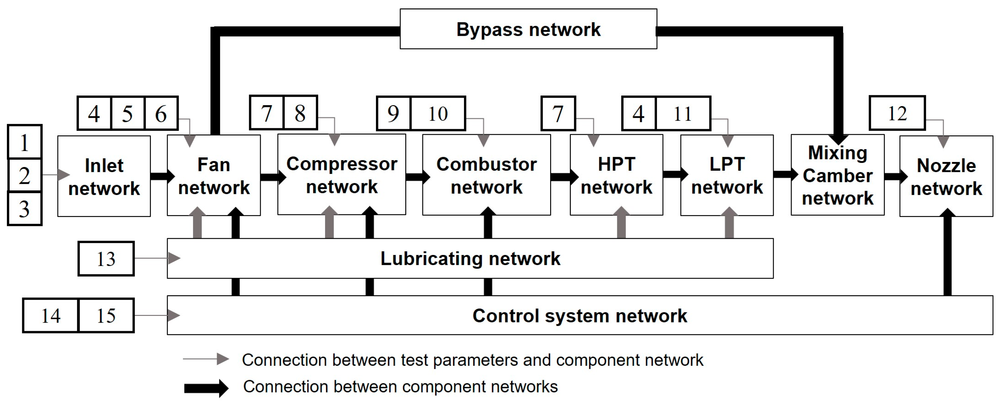
The specific engine digital model consisted of 11 independent learning networks, including the inlet, fan, compressor, combustor, high-pressure turbine (HPT), low-pressure turbine (LPT), mixing chamber, nozzle, bypass, lubricating, and control system networks. The order in which air flows through the components in the physical space mirrors the data transmission relationship among independent learning networks in the digital space, as shown in Figure 7. Furthermore, as discussed above, the data link relationships for the control system, lubricating, and bypass networks corresponded one-to-one to the physical aircraft engine. The selected features were then sent to the corresponding networks. All the independent component networks used the LSTM network, with all LSTM networks configured to have 12 output nodes, to consider the influence of the time series in this case study.
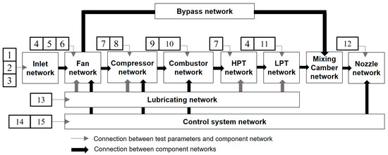
Figure 7.
Two-shaft mixed turbofan engine digital model.
Next, a regression model was added to correlate the aircraft engine performance in the digital space with the target parameters. The inputs to the regression model were the outputs of the component networks corresponding to the exhaust components of the aircraft engine in physical space. For example, a turbofan engine with split flow will exhaust the core and bypass flows into the atmosphere through main and bypass nozzles, respectively. Consequently, two output features were produced by the corresponding networks and sent to the regression model. In contrast, the regression model only received the features produced by the nozzle network for a mixed exhaust turbofan engine. The regression model was a fully connected network; that is, any node in the n − 1th layer was connected to all nodes in the nth layer.
The inputs for each component network within the model must be set to transfer the engine components from physical to digital space matching after the deep learning architecture of a specific digital model is established. External and internal inputs exist for each component network. The external inputs consist of relevant parameters that express the characteristics of the components. Internal inputs are formed by the data transmission relationship between the component networks. For example, measured features include the fuel flow and low- and high-pressure rotor speeds. However, only the low-pressure rotor speed expresses the characteristics of a fan. In addition, a component network in the digital space reads the input that expresses the characteristics of the component. Moreover, many types of features can be measured for a component but not all are related to the target parameter. From the perspective of association, the exhaust gas temperature (as the target parameter) is directly related to the environmental, engine state, and control parameters. These parameters were utilized as external inputs for the component networks within the model.
This study used a dataset that included six flight and four engine test records provided by the Civil Aviation Flight University of China. The records included the atmospheric humidity, rotational speeds of the high- and low-pressure shafts, angle of the guide vane, total temperature, and total pressure at the component section. The data listed in Table 1 were selected as external inputs for the component networks in the case study. In the table, the numbers in the index columns correspond to those in Figure 7 and represent the position of the input features. The abbreviations HP, LP, and PL indicate high-pressure, low-pressure, and pressurizing lines, respectively.

Table 1.
Selected features for the component input.
Different indicators have different dimensions and value ranges. The gradient of the model along different directions changes significantly if the data are directly input into the model for training, making convergence difficult. Therefore, it is necessary to normalize and scale the data of all dimensions to the range of [0, 1], which can accelerate the convergence speed and improve the prediction accuracy. The min–max method was used to standardize the data, which is expressed as:
where x and x* denote the original and standardized data, respectively. xmin and xmax represent the minimum and maximum values for each dataset, respectively. The output of the model was inversely normalized to obtain the predicted exhaust gas temperature after completing the model training with the standardized data. The mean square error (MSE) was selected as the loss function of the model during the training process, which is expressed as:
where yi denotes the standardized target data, f(xi) denotes the regression model output, and N denotes the training sample size. The training process was iterative with two stages: forward and back propagation. During forward propagation the input data were passed in specific directions in digital space, representing one-way links between different nodes in the neural network model. After the computation occurred at the nodes, the output of the regression model was obtained and used to calculate the iteration errors using the loss function. Back propagation occurred when the errors (as input) passed along the opposite direction of the forward propagation. The coefficients and weights were adjusted based on the contributions of the nodes to the error. The training ended when the error met the accuracy criterion or the number of specified iterations in the round was reached.
The model training parameters initialization is detailed in Table 2. In Table 2, batch size is the number of data points utilized in each iteration of training in a neural network. Epoch is the occurrence of a complete pass through the entire training dataset during the training of a machine learning model. The training process was conducted five times at a fixed model capacity defined by a specific number of nodes, resulting in five distinct digital engine models. Each model was utilized to predict EGT based on the provided input values. Subsequently, the performance metrics of these five digital models were aggregated and measured to comprehensively assess their predictive capabilities. The evaluation was based on the average relative error (ARE), which is expressed as:
where Ym denotes the digital model output, Yr denotes the test target experimental data, and N denotes the testing sample size.
Table 2.
Configuration of Model Training Parameters.
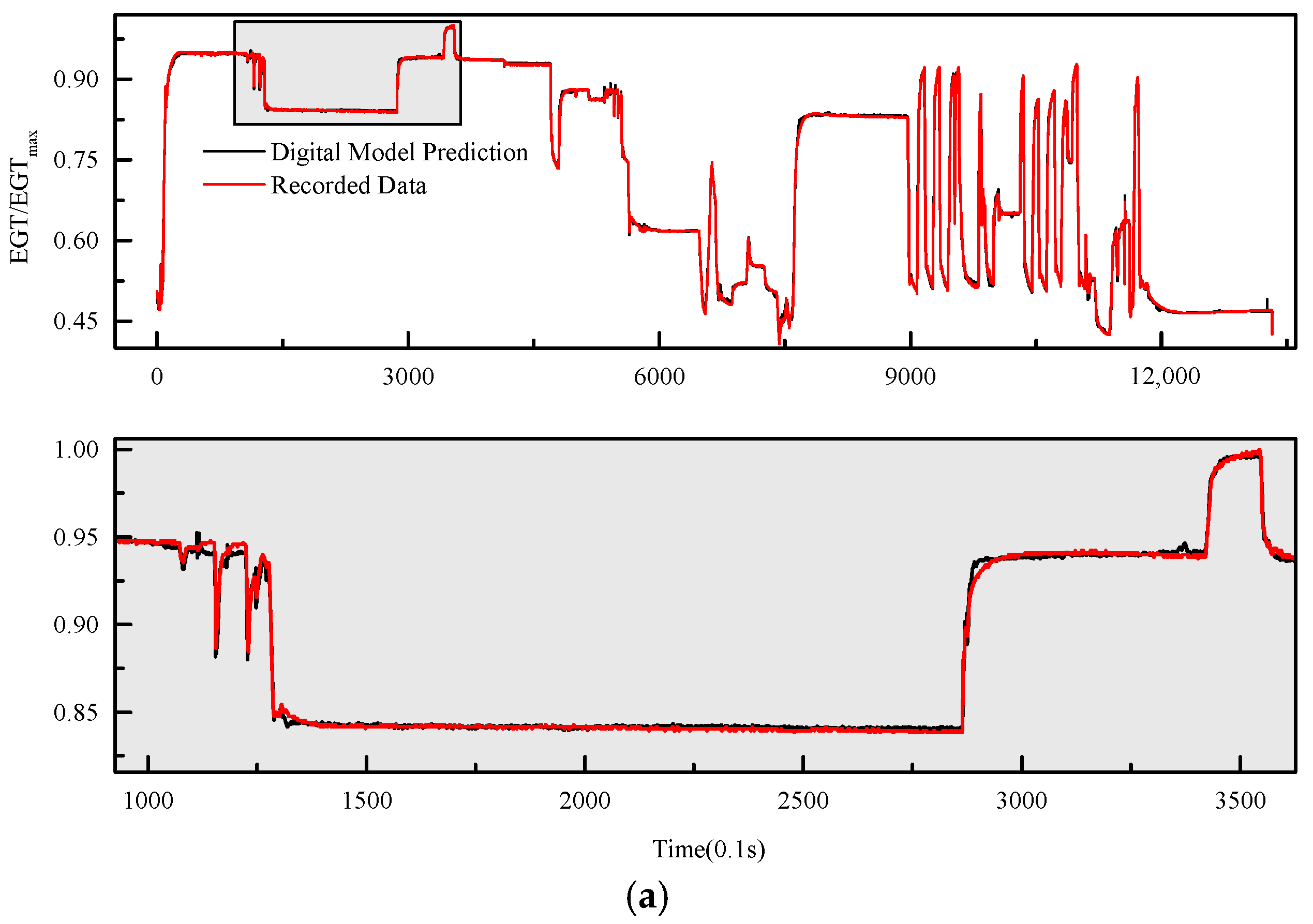
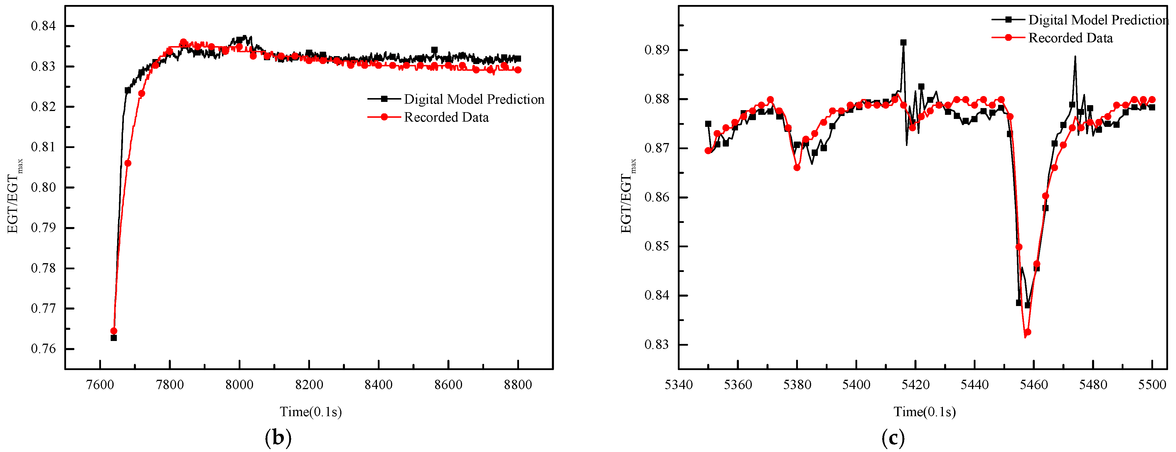
The test results of the digital engine model performance on two separate testing datasets are listed in Table 3. Additionally, experiments were conducted on testing dataset 2 with different model capacities to explore their impact on predictive accuracy. Figure 8 and Figure 9, respectively, showcase the model performance for real-time prediction of EGT on two testing datasets. The digital engine model effectively and accurately predicted the EGT during steady- and unsteady-state conditions, making it a reliable method for real-time EGT predictions. This is demonstrated by the ARE of models DM_1 and DM_2 in Table 3, as well as in Figure 8 and Figure 9. In the zoom-ins of Figure 8 and Figure 9a, it is evident that the model incurs significant EGT prediction errors during engine slow-speed and unsteady-state conditions, especially at positions where the engine initiates acceleration or deceleration. These errors arise from two main factors, namely fluctuations in EGT sensor measurement during such states and the presence of latency in the model’s real-time predictions.
Table 3.
Results of the digital model on testing datasets.
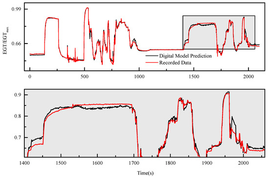
Figure 8.
Performance of the digital model on testing dataset 1.
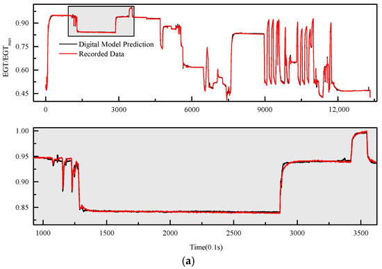
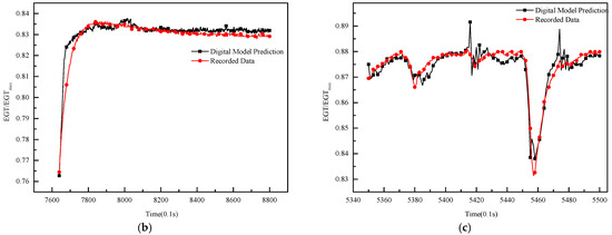
Figure 9.
Performance of the digital model on testing dataset 2. (a) All engine state conditions. (b) Unsteady- to steady-state conditions [7640, 8800]. (c) Unsteady-state conditions [5350, 5500].
In the DM_2-2 and DM_2-3, the number of output nodes for their independent component networks is 10 and 9, respectively. In the context of DM_2-1, DM_2-2, and DM_2-3 models, DM_2-1 exhibits the largest model capacity, followed by DM_2-2, and DM_2-3 possesses the smallest capacity. A comparison of the model performance with different capacities on testing dataset 2 indicates that reducing model capacity results in an increased standard deviation, signifying a decrease in stability. But the models still demonstrate effective predicting of the EGT under both steady- and unsteady-state conditions, as evidenced by the ARE of the models.
5.2. Real-Time Prediction of the Total Pressure
The real-time prediction of the total pressure at the compressor exit was considered in the second case study. This case highlights the versatility of the presented architecture for parameter prediction, demonstrating that the architecture enabled accurate prediction of the performance parameters of the entire engine and facilitated the acquisition of performance parameters for individual components within the engine system. This distinction is essential because the behavior of an engine component may differ when operating as part of a complete engine assembly compared with its isolated performance in numerical simulations.
The constant demand for performance improvements in aircraft engines has led to attempts to advance compressor technology to achieve superior performance. Increasing the compressor pressure ratio is one method to improve engine performance. However, this renders the compressor unstable. The instability indicator usually considers dynamic parameters, such as pressure, vibration, temperature, and rotational speed. The total pressure fluctuates sharply when the compressor becomes unstable. Therefore, the total pressure at the compressor exit is typically used for monitoring engine operation.
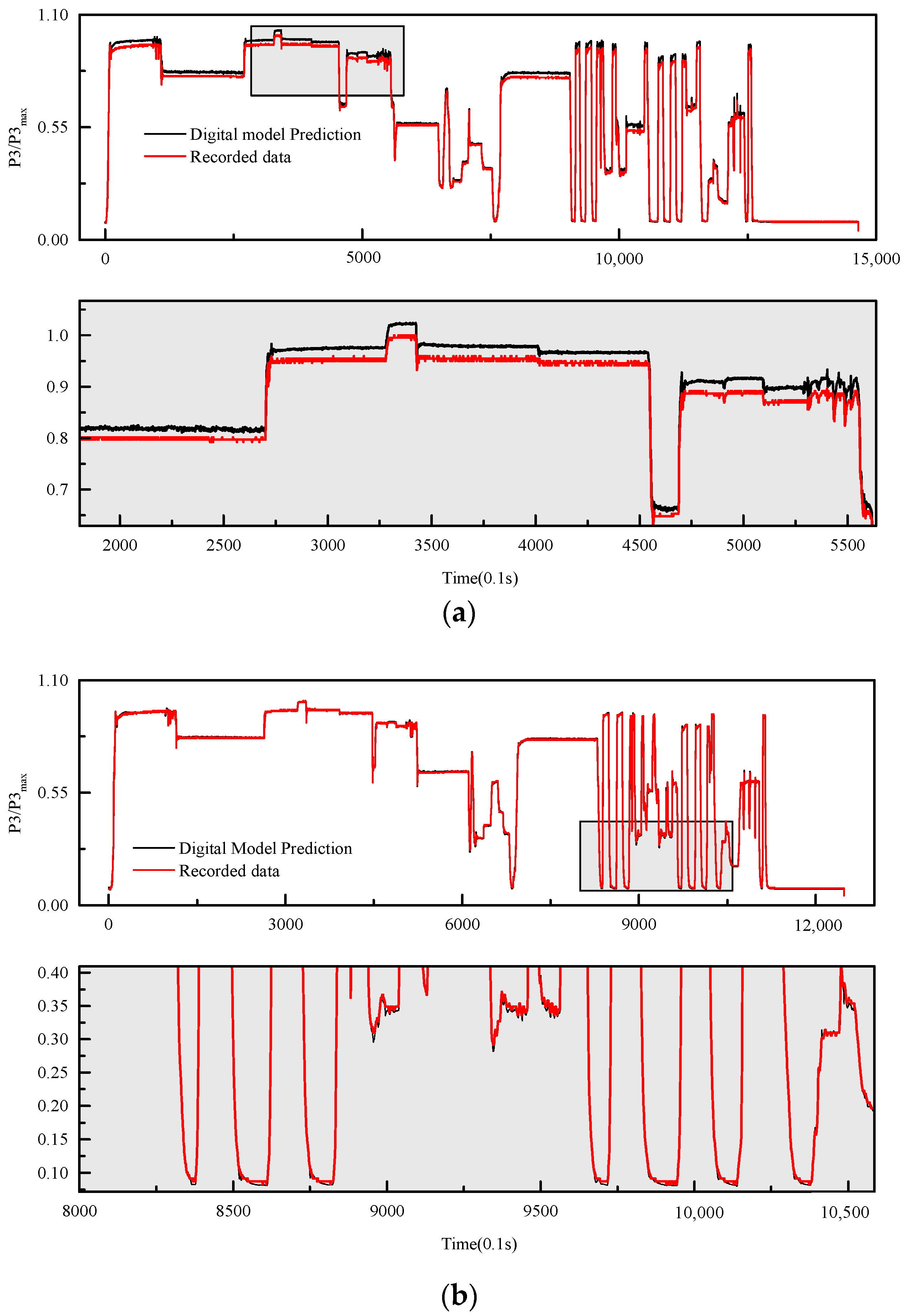
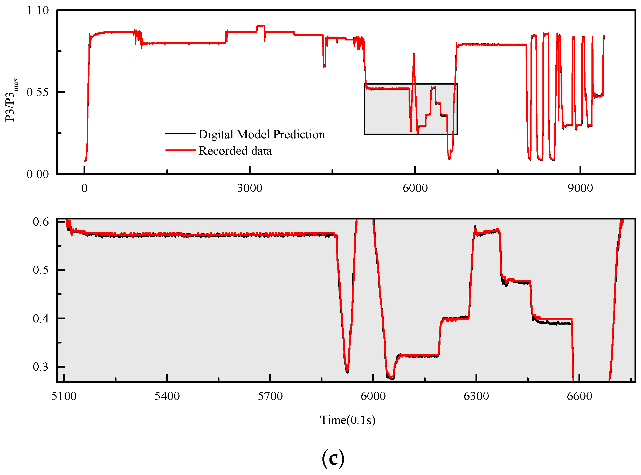
The digital model architecture and process for predicting the total pressure at a compressor outlet were consistent with those described in the first case study, except the total pressure at the combustor inlet from the input parameters was excluded. The digital model obtained from the training data was validated under different flight missions, and the results are listed in Table 4. The model performance for these flight missions is illustrated in Figure 10. The results demonstrated that the digital model consistently and accurately predicted the cross-sectional parameter of the compressor in real-time during the engine slow-speed, intermediate, maximum, acceleration, and deceleration state conditions. Comparing the model performance across the three engine flight missions, as shown in Figure 10, it is evident that the model incurs large prediction errors when the engine initiates acceleration/deceleration. This situation is particularly pronounced in flight mission 1. It is observed from Figure 10a that errors of model prediction in engine unsteady-state conditions impact the model prediction in engine steady-state conditions, leading to an increase in model prediction error in engine steady-state conditions. This discrepancy stems from the normalization of training data to a specific range. The represented engine performance of flight mission 1 experiences a relative degradation compared with the engine performance depicted in the training dataset. Consequently, the model prediction in flight mission 1 manifests an overestimation relative to the recorded parameter value.
Table 4.
Results of the digital model on three flight conditions.
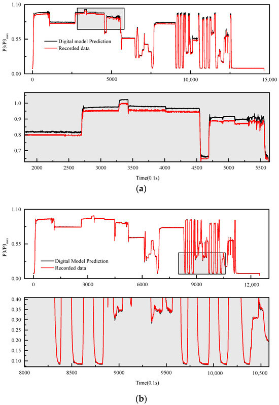
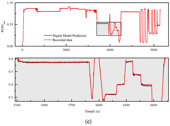
Figure 10.
Performance of the digital model on three flight missions. (a) Flight mission 1. (b) Flight mission 2. (c) Flight mission 3.
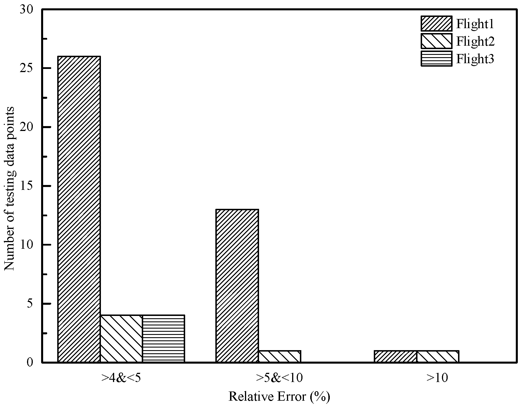
Insights into the number of testing data points where the digital model exhibited large prediction errors are provided in Figure 11. The height of the bar in Figure 11 represents the number of testing data points, and the horizontal coordinates are the ARE of the model predicting parameter. Analyzing both Figure 10 and Figure 11 alongside the MRE of the model in three flight missions, it is evident that data points with significant errors in real-time model predictions are rare, accounting for less than 0.3% of the total prediction testing data points. When comparing Figure 10b,c, the model exhibits a higher MRE in real-time parameter prediction for flight mission 2. This can be attributed to the small numerical values in the recorded testing data, leading to a notable increase in the MRE due to the small denominator when calculating the relative error.
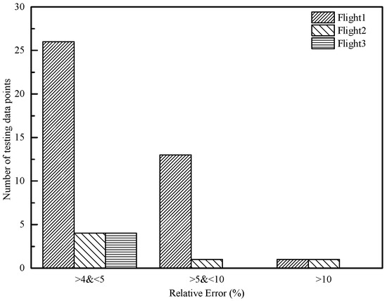
Figure 11.
Histogram of prediction error statistics of the digital model for three flight missions.
5.3. Real-Time Performance Degradation Comparison
The application of parameter prediction to analyze the performance degradation of aircraft engines was considered in the third case study. This case study was designed to highlight the features of a digital engine model, which was utilized to address aircraft engine engineering problems that were difficult to address using conventional methods. Aircraft engine performance is crucial to ensure successful flight missions. However, variations in manufacturing and assembly tolerances can lead to differences in aircraft engine performance. Additionally, engine performance changes over its lifetime owing to the degradation and recovery processes, further affecting its overall performance. Therefore, it is imperative to measure the extent of performance change caused by the engine lifespan to assess whether it meets flight requirements.
The EGT is commonly used as an aircraft engine performance metric to evaluate the degradation of an aircraft engine in real time. The gas temperature decreases after the gas works on the turbine. The lower the EGT, the more the gas has worked on the turbine. A higher than standard range EGT is a warning sign for aircraft engine health. Thus, a change in EGT represents a change in the aircraft engine performance. In general, the EGT at the maximum operating condition (often referred to as the peak state) is meticulously recorded and compared with the EGT at the peak state of the previous flight. This practice serves as a critical indicator for evaluating engine performance degradation. Nonetheless, this assessment presents a multifaceted challenge because of the significant influence of diverse factors, including flight missions, intricate control laws governing engine behavior, and ever-changing external environmental conditions. Consequently, the comparison of EGT inherently involves different flight states, introducing complexities into the analysis. In addition, the presence of an unidentified engine model in a degraded state poses challenges for traditional numerical simulation methods to assess the EGT.
Obtaining the performance parameters in a consistent operating state before and after a change in engine performance forms the basis for evaluating performance degradation. To address this, an approach involving the construction of two distinct digital engine models was presented representing the engine before and after performance degradation. Preservation of the engine characteristics within the corresponding timeframe of the data was ensured by carefully crafting the engine digital model with appropriate data. Subsequently, both digital models were fed identical datasets to predict the performance parameters and the digital engine models executed simulations based on the given flight states and control law.
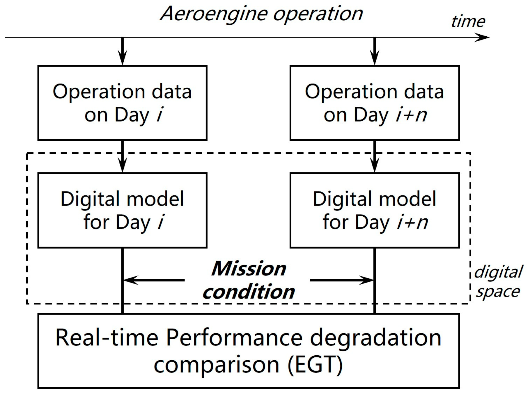
The process of comparing engine performance degradation based on real-time EGT predictions is depicted in Figure 12. Two sets of operational data were available for an aircraft engine corresponding to the ith and i + nth days. For this analysis, it was assumed that the aircraft engine did not undergo any maintenance or performance recovery during its period of use. Two distinct digital models were meticulously mapped using the aforementioned datasets by leveraging the given architecture. These digital models were designed to encapsulate the engine behavior under specific mission conditions, encompassing the operating environment and aircraft engine state. As such, the model functionality was driven by a combination of essential data, including environmental, engine state, and control parameters. Subsequently, a digital experiment was conducted for performance comparison where both digital models were executed under identical mission conditions, and real-time EGT predictions were made. The essence of the performance degradation was assessed by carefully scrutinizing and contrasting the EGT values predicted by the two digital models.
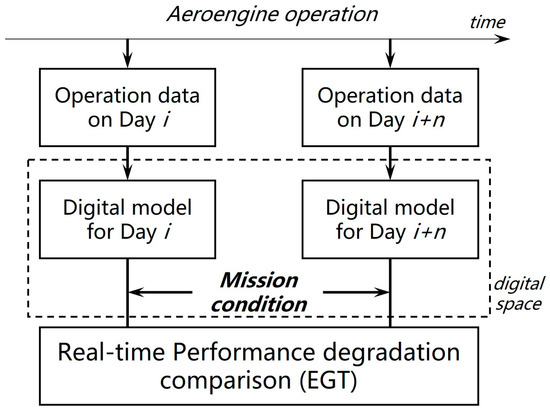
Figure 12.
Process of comparison degradation in aircraft engine performance (EGT).
Unlike the first case study, the third case study utilized flight data from the engine, resulting in a more limited availability of the parameters. This limitation arose because of the constraints of the airborne environment, where the total aircraft engine load was restricted and the arrangement of sensors on the engine during flight was significantly lower than that of the extensive sensor setup utilized in aircraft engine testing. Consequently, the features selected for the digital model in this case study were limited to those that were measurable during airborne operations. One of the most noticeable effects was a reduction in the cross-sectional aerodynamic parameters of certain components. The selected parameters mainly include the air temperature, flight altitude, inlet guide vane angle, rotor speed, area of nozzle throat, oil pressure, throttle position, and afterburner switch. Similarly, all the independent component networks used the LSTM network, with all LSTM networks configured to have 12 output nodes.
The smaller the EGT predicted by the model, the better the corresponding aircraft engine performance. Theoretically, the EGT predicted by the digital model on day i was expected to be lower than that predicted on day i + n under the same mission conditions. This result was consistent with the discussion above. The architectures of the two digital models in the demonstration were consistent with those in the first case study. The two digital models represented the states of the aircraft engine after three (baseline model) and six flights. The baseline model mostly predicted lower exhaust gas temperatures in real time when compared with the other model. Figure 13 illustrates the real-time EGT prediction of two digital models representing engine performance at different runtimes. The black curve represents the predicted EGT values by the digital model for an engine with short runtimes, while the red one represents the predicted EGT values by the digital model for an engine with long runtimes. As depicted in Figure 13, the values of the former are lower than those of the latter. Performance degradation was quantified by averaging the predictions of the two models under steady-state conditions and then computing their differences. The errors arising from the digital model training affect the assessment of engine performance degradation. To mitigate the impact of these errors on the calculation of performance degradation, the evaluation method is expressed as:
where Δ denotes the performance metric to evaluate the engine performance degradation, Δo denotes the difference between the two models under steady-state conditions, and Me denotes the model correction. The model correction is equal to the absolute average of the difference between the model-predicted values and the recorded testing values.
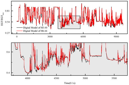
Figure 13.
Comparison of performance prediction of engine digital models representing different states.
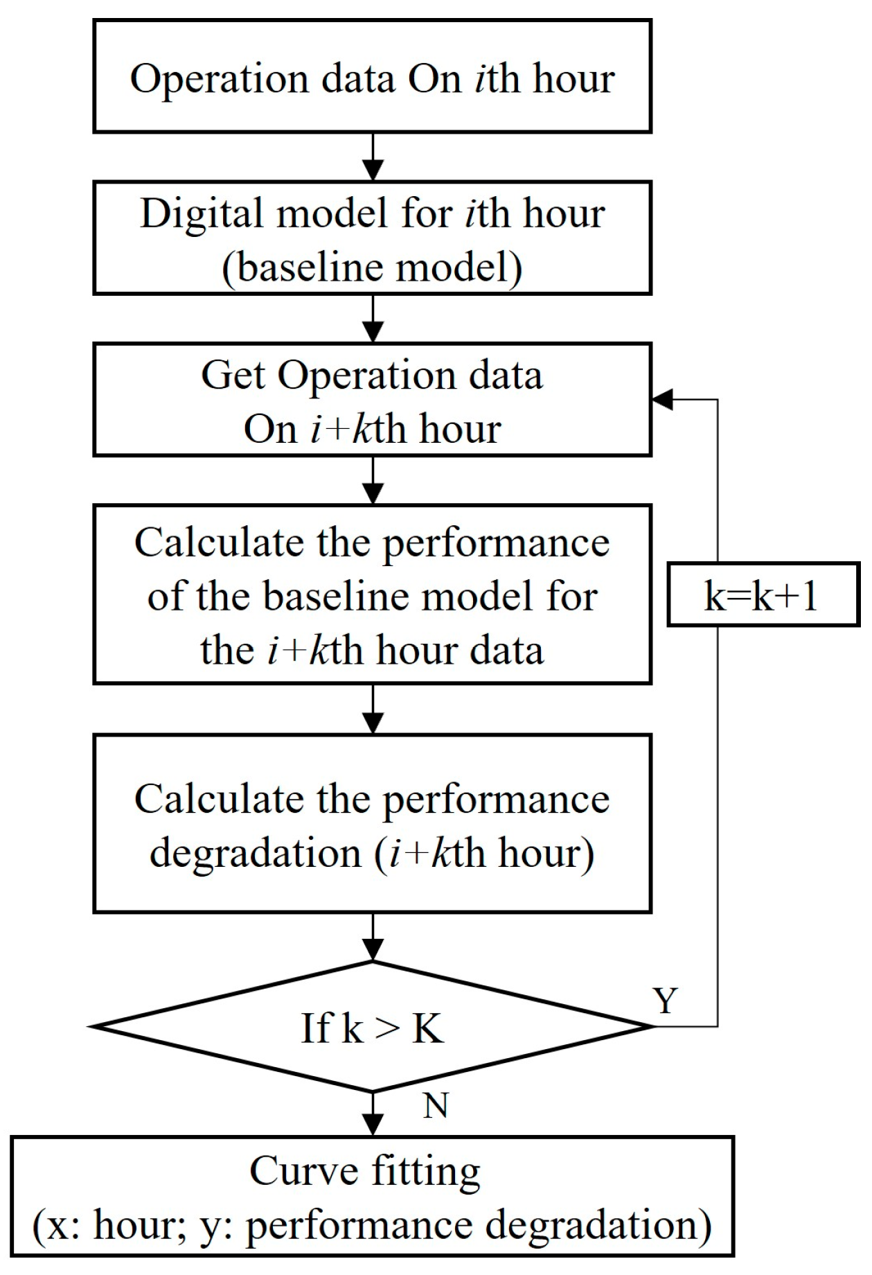
The above process was repeated to obtain the engine performance degradation curve, which illustrated the changes in engine performance over its operating time. To simplify the process, a digital model was generated by training the engine with data from its initial state. Subsequent flight data were then sequentially fed into the digital model to predict the engine performance parameters under specific operating conditions corresponding to the initial state. The extent of performance degradation was determined by comparing the experimental and predicted EGT during the same flight sorties. The specific flow is shown in Figure 14.
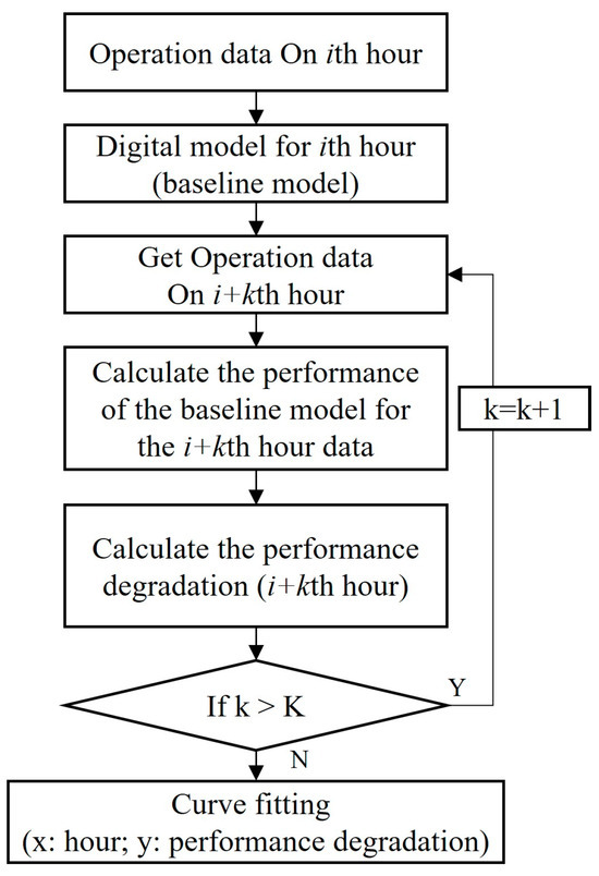
Figure 14.
Process for obtaining engine performance degradation curves.
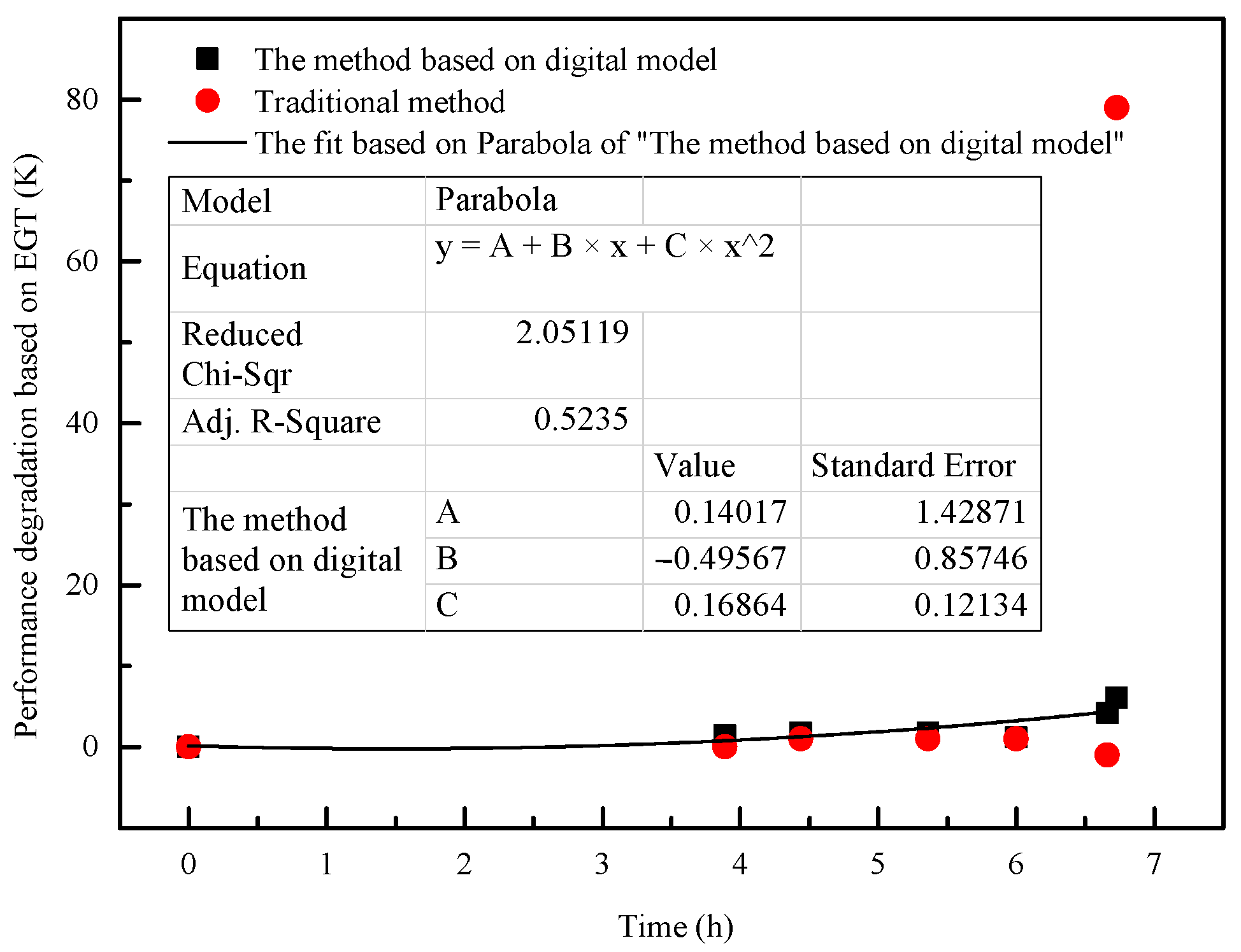
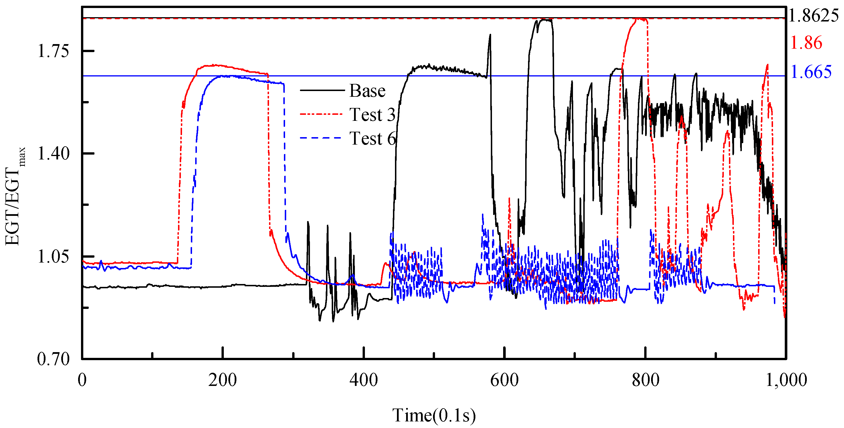
A performance degradation prediction result based on six flight testing data is presented in Table 5, and the performance degradation prediction curve is shown in Figure 15. In Table 5, ‘Testing’ represents flight testing data, and ‘Base’ serves as the baseline for engine performance degradation evaluation. ΔT denotes the degradation evaluation calculated using the traditional method. ΔD denotes the degradation evaluation calculated using the digital model-based method presented in this study. The traditional method evaluates engine performance degradation by measuring the difference in performance metrics at the engine’s maximum state condition. The graph illustrates a gradual decline in engine performance over time. From Figure 15, it is evident that traditional methods exhibit significant deviations when predicting the performance degradation of ‘Test 6’. Figure 16 provides the EGT values of flight testing, along with the maximum recorded data. Figure 16 reveals a significant disparity in the testing data of ‘Test 6’, leading to the ineffectiveness of the traditional method. In contrast, the performance degradation evaluation based on the digital model is not constrained by the engine flight mission and provides a more effective prediction of the evaluation of engine performance degradation. Moreover, it is essential to note that achieving more accurate results requires additional engine operational data and a more detailed experimental design. Addressing these aspects will be a key focus of future efforts to improve and refine performance predictions.
Table 5.
The results of the engine performance degradation based on EGT.
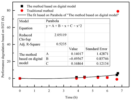
Figure 15.
Parabola fit of degradation based on EGT.

Figure 16.
EGT value of the flight testing.
6. Conclusions
Predicting the fluid properties in complex flow through thermodynamic machinery is a common problem in engineering. Some complex flows have been investigated by classic hydrodynamic studies using either the Navier–Stokes–Fourier framework or the molecular-level method. Most researchers caution that investigating complex flow is challenging.
This study introduced physics-embedded deep learning as a novel approach for predicting real-time fluid properties in complex flow. This method leveraged a domain decomposition approach to represent complex mechanical systems, specifically aircraft engines, in digital space using physics-embedded deep learning. Each engine component, including the inlet, fan, and compressor, was modeled as an independent learning network, and data transmission relationships were established to simulate their interactions. The architecture was validated through two case studies for EGT and the predicted total pressure at the compressor outlet in aircraft engines. The two parameters respectively represent the overall performance and component performance of the engine. Accurate and efficient performance was demonstrated using engine testing data. Moreover, an advantage of the presented method is its capability to address complex aero-engineering problems that are traditionally challenging to solve, thus offering valuable insights. In the case of engine performance degradation, the engine deteriorates, leading to changes in the physical equations describing engine operation. As the method does not directly rely on the physical equations that describe the complex thermodynamic machinery, it can more efficiently predict the aerodynamic parameters of the engine under degraded conditions. Finally, the presented approach promotes safety and efficiency in the aerospace industry.
In this study, real-time prediction refers to the timely prediction of complex flow parameters during the operation of thermodynamic machinery. This is achieved by continuously inputting sensor data into the model. For this study, the parameter prediction was executed within the engine onboard computer, utilizing the i7-6820EQ CPU to emulate the operational setting. Real-time data transmission operates at a frequency of 50 Hz, requiring parameter prediction to be completed within 20 ms. Within the computational environment, the time of the model loading and real-time predictions for one data record is 6 s and 0.013 s, respectively. The time for real-time prediction meets the demands of the onboard computational environment. It is crucial to note that the time spent on real-time parameter prediction is predominantly influenced by the component network, and more intricate networks may necessitate additional time.
Author Contributions
Methodology, software, visualization, writing—original draft preparation, Z.L.; methodology, data curation, writing—original draft preparation, H.X.; data curation, visualization, writing—reviewing and editing, D.X. All authors have read and agreed to the published version of the manuscript.
Funding
This research was funded by the National Natural Science Foundation of China, grant number 52076180; National Science and Technology Major Project, grant number J2019-I-0021-0020; Science Center for Gas Turbine Project, grant number P2022-B-I-005-001; The Fundamental Research Funds for the Central Universities.
Data Availability Statement
The data that support the findings of this study are available from the corresponding author, Hong Xiao, upon reasonable request.
Acknowledgments
Zhifu Lin and Dasheng Xiao contributed equally to this work. Special thanks go to R. S. Myong of Gyeongsang National University, Republic of Korea, for his helpful discussions.
Conflicts of Interest
The authors declare no conflicts of interest.
References
- Yarom, E.; Sharon, E. Experimental observation of steady inertial wave turbulence in deep rotating flows. Nat. Phys. 2014, 10, 510. [Google Scholar] [CrossRef]
- Barkley, D.; Song, B.; Mukund, V.; Lemoult, G.M.; Hof, A.B. The rise of fully turbulent flow. Nature 2015, 526, 550. [Google Scholar] [CrossRef]
- Bauer, P.; Thorpe, A.; Brunet, G. The quiet revolution of numerical weather prediction. Nature 2015, 525, 47–55. [Google Scholar] [CrossRef]
- Falkovich, G.; Sreenivasan, K.R. Lessons from hydrodynamic turbulence. Phys. Today 2006, 59, 43–49. [Google Scholar] [CrossRef]
- Ozawa, H.; Shimokawa, S.; Sakuma, H. Thermodynamics of fluid turbulence: A unified approach to the maximum transport properties. Phys. Rev. E 2001, 64, 026303. [Google Scholar] [CrossRef]
- Righi, M.; Pachidis, V.; Konozsy, L.; Giersch, T.; Schrape, S. Experimental validation of a three-dimensional through-flow model for high-speed compressor surge. Aerosp. Sci. Technol. 2022, 128, 107775. [Google Scholar] [CrossRef]
- LeCun, Y.; Bengio, Y.; Hinton, G. Deep learning. Nature 2015, 521, 436–444. [Google Scholar] [CrossRef]
- Sarker, I.H. Deep learning: A comprehensive overview on techniques, taxonomy, applications and research directions. SN Comput. Sci. 2021, 2, 420. [Google Scholar] [CrossRef] [PubMed]
- Schmidhuber, J. Deep learning in neural networks: An overview. Neural Netw. 2015, 61, 85–117. [Google Scholar] [CrossRef] [PubMed]
- Senior, A.W.; Evans, R.; Jumper, J.; Kirkpatrick, J.; Sifre, L.; Green, T.; Qin, C.; Žídek, A.; Nelson, A.W.R.; Bridgland, A.; et al. Improved protein structure prediction using potentials from deep learning. Nature 2020, 577, 706–710. [Google Scholar] [CrossRef] [PubMed]
- Devlin, J.; Chang, M.W.; Lee, K.; Toutanova, K. Bert: Pre-training of deep bidirectional transformers for language understanding. arXiv 2018, arXiv:1810.04805. [Google Scholar]
- Rajkomar, A.; Oren, E.; Chen, K.; Dai, A.M.; Hajaj, N.; Hardt, M.; Liu, P.J.; Liu, X.; Marcus, J.; Sun, M.; et al. Scalable and accurate deep learning with electronic health records. NPJ Digit. Med. 2018, 1, 18. [Google Scholar] [CrossRef] [PubMed]
- Chen, Y.; Wang, S.; Liu, W. Data-Driven Transition Models for Aeronautical Flows with a High-Order Numerical Method. Aerospace 2022, 9, 578. [Google Scholar] [CrossRef]
- Xie, C.; Wang, J.; Li, K.; Ma, C. Artificial neural network approach to large-eddy simulation of compressible isotropic turbulence. Phys. Rev. E 2019, 99, 053113. [Google Scholar] [CrossRef] [PubMed]
- Dong, Y.; Liao, F.; Pang, T.; Su, H.; Zhu, J.; Hu, X.; Li, J. Boosting adversarial attacks with momentum. In Proceedings of the IEEE Conference on Computer Vision and Pattern Recognition 2018, Salt Lake City, UT, USA, 18–21 June 2018. [Google Scholar]
- Rauker, T.; Ho, A.; Casper, S.; Hadfield-Menell, D. Toward transparent ai: A survey on interpreting the inner structures of deep neural networks. In Proceedings of the 2023 IEEE Conference on Secure and Trustworthy Machine Learning (SaTML), San Francisco, CA, USA, 8–10 February 2023. [Google Scholar]
- Xu, F.; Uszkoreit, H.; Du, Y.; Fan, W.; Zhao, D.; Zhu, J. Explainable ai: A brief survey on history, research areas, approaches and challenges. In Proceedings of the Natural Language Processing and Chinese Computing: 8th CCF International Conference, NLPCC 2019, Dunhuang, China, 9–14 October 2019. [Google Scholar]
- Haakon, R.; Suraj, P.; Adil, R.; Omer, S. Physics guided neural networks for modelling of non-linear dynamics. Neural Netw. 2022, 154, 333–345. [Google Scholar]
- Amos, B.; Kolter, J.Z. OptNet: Differentiable optimization as a layer in neural networks. arXiv 2021, arXiv:1703.00443. [Google Scholar]
- Pang, G.; D’Elia, M.; Parks, M.; Karniadakis, G.E. nPINNs: Nonlocal physics-informed neural networks for a parametrized nonlocal universal Laplacian operator. Algorithms and applications. J. Comput. Phys. 2020, 422, 109760. [Google Scholar] [CrossRef]
- Zanardi, I.; Venturi, S.; Panesi, M. Adaptive physics-informed neural operator for coarse-grained non-equilibrium flows. Sci. Rep. 2023, 13, 15497. [Google Scholar] [CrossRef]
- Xu, C.; Yongjie, F.; Shuo, L.; Xuan, D. Physics-Informed Neural Operator for Coupled Forward-Backward Partial Differential Equations. In Proceedings of the 1st Workshop on the Synergy of Scientific and Machine Learning Modeling ICML2023, Honolulu, HI, USA, 28 July 2023. [Google Scholar]
- Zobeiry, N.; Humfeld, K.D. A physics-informed machine learning approach for solving heat transfer equation in advanced manufacturing and engineering applications. Eng. Appl. Artif. Intell. 2021, 101, 104232. [Google Scholar] [CrossRef]
- Arnold, F.; King, R. State-space modeling for control based on physics-informed neural networks. Eng. Appl. Artif. Intell. 2021, 101, 104195. [Google Scholar] [CrossRef]
- Shinjan, G.; Amit, C.; Georgia, O.B.; Biswadip, D. RANS-PINN based Simulation Surrogates for Predicting Turbulent Flows. In Proceedings of the 1st Workshop on the Synergy of Scientific and Machine Learning Modeling ICML2023, Honolulu, HI, USA, 28 July 2023. [Google Scholar]
- Balli, O.; Caliskan, H. Turbofan engine performances from aviation, thermodynamic and environmental perspectives. Energy 2021, 232, 121031. [Google Scholar] [CrossRef]
- Tsoutsanis, E.; Li, Y.G.; Pilidis, P.; Newby, M. Part-load performance of gas turbines: Part I—A novel compressor map generation approach suitable for adaptive simulation. In Proceedings of the ASME Gas Turbine India Conference 2012, Mumbai, India, 1–3 December 2012. [Google Scholar]
- Tsoutsanis, E.; Li, Y.G.; Pilidis, P.; Newby, M. Part-load performance of gas turbines: Part II-Multi-point adaptation with compressor map generation and ga optimization. In Proceedings of the ASME Gas Turbine India Conference 2012, Mumbai, India, 1–3 December 2012. [Google Scholar]
- Liu, J.; Zhang, Q.; Pei, J.; Tong, H.; Feng, X.; Wu, F. Fsde: Efficient evolutionary optimization for many-objective aero-engine calibration. Complex Intell. Syst. 2022, 8, 2731–2747. [Google Scholar] [CrossRef]
- Flack, R.D. Fundamentals of Jet Propulsion with Applications; Cambridge University Press: Cambridge, UK, 2005; Volume 17. [Google Scholar]
- Pinto, R.N.; Afzal, A.; D’Souza, L.V.; Ansari, Z.; Mohammed Samee, A. Computational fluid dynamics in turbomachinery: A review of state of the art. Arch. Comput. Methods Eng. 2017, 24, 467–479. [Google Scholar] [CrossRef]
- Goodfellow, I.; Bengio, Y.; Courville, A. Deep Learning; MIT Press: Cambridge, MA, USA, 2016. [Google Scholar]
- Nagarajan, V. Explaining generalization in deep learning: Progress and fundamental limits. arXiv 2021, arXiv:2110.08922. [Google Scholar]
- Karniadakis, G.E.; Kevrekidis, I.G.; Lu, L.; Perdikaris, P.; Wang, S.; Yang, L. Physics-informed machine learning. Nat. Rev. Phys. 2021, 3, 422–440. [Google Scholar] [CrossRef]
- Elattar, H.M.; Elminir, H.K.; Riad, A.M. Towards online data-driven prognostics system. Complex Intell. Syst. 2018, 4, 271–282. [Google Scholar] [CrossRef]
- Tartakovsky, A.M.; Marrero, C.O.; Perdikaris, P.; Tartakovsky, G.D.; Barajas-Solano, D. Physics-informed deep neural networks for learning parameters and constitutive relationships in subsurface flow problems. Water Resour. Res. 2020, 56, e2019WR026731. [Google Scholar] [CrossRef]
- Yang, L.; Zhang, D.; Karniadakis, G.E. Physics-informed generative adversarial networks for stochastic differential equations. SIAM J. Sci. Comput. 2020, 42, 292–317. [Google Scholar] [CrossRef]
- Raissi, M.; Perdikaris, P.; Karniadakis, G.E. Physics-informed neural networks: A deep learning framework for solving forward and inverse problems involving nonlinear partial differential equations. J. Comput. Phys. 2019, 378, 686–707. [Google Scholar] [CrossRef]
- Han, J.; Jentzen, A.; Weinan, E. Solving high-dimensional partial differential equations using deep learning. Proc. Natl. Acad. Sci. USA 2018, 115, 8505–8510. [Google Scholar] [CrossRef]
- Han, J.; Jentzen, A.; Ee, W. Deep learning-based numerical methods for high-dimensional parabolic partial differential equations and backward stochastic differential equations. Commun. Math. Stat. 2017, 5, 349–380. [Google Scholar]
- Sirignano, J.; Spiliopoulos, K. DGM: A deep learning algorithm for solving partial differential equations. J. Comput. Phys. 2018, 375, 1339–1364. [Google Scholar] [CrossRef]
- Wigstrom, H. A neuron model with learning capability and its relation to mechanisms of association. Kybernetik 1973, 12, 204–215. [Google Scholar] [CrossRef] [PubMed]
- Gers, F.A.; Schmidhuber, J.; Cummins, F. Learning to forget: Continual prediction with lstm. Neural Comput. 2000, 12, 2451–2471. [Google Scholar] [CrossRef]


Disclaimer/Publisher’s Note: The statements, opinions and data contained in all publications are solely those of the individual author(s) and contributor(s) and not of MDPI and/or the editor(s). MDPI and/or the editor(s) disclaim responsibility for any injury to people or property resulting from any ideas, methods, instructions or products referred to in the content. |
© 2024 by the authors. Licensee MDPI, Basel, Switzerland. This article is an open access article distributed under the terms and conditions of the Creative Commons Attribution (CC BY) license (https://creativecommons.org/licenses/by/4.0/).