
Reinforcement Learning for Dual-Control Aircraft Six-Degree-of-Freedom Attitude Control with System Uncertainty
School of Astronautics, Harbin Institute of Technology, Harbin 150001, China
*
Author to whom correspondence should be addressed.
Aerospace 2024, 11(4), 281; https://doi.org/10.3390/aerospace11040281
Submission received: 7 February 2024
/
Revised: 20 March 2024
/
Accepted: 2 April 2024
/
Published: 4 April 2024
Abstract
:This article proposes a near-optimal control strategy based on reinforcement learning, which is applied to the six-degree-of-freedom (6-DoF) attitude control of dual-control aircraft. In order to solve the problem that the existing reinforcement learning is difficult to apply to the high-dimensional multiple-input multiple-output (MIMO) systems, the Long Short-Term Memory (LSTM) neural network is introduced to replace the polynomial network in the adaptive dynamic programming (ADP) technique. Meanwhile, based on the Lyapunov method, a novel online adaptive updating law of LSTM neural network weights is given, and the stability of the system is verified. In the simulation process, the algorithm proposed in this article is applied to the six-degree-of-freedom attitude control problem of dual-control aircraft with system uncertainty. The simulation results show that the algorithm can achieve near-optimal control.
1. Introduction
Aircraft attitude control is an important part of the design of aircraft autopilot. With the increase in aircraft flying altitude and speed, pure aerodynamic control has been unable to meet the tracking requirements of attitude control commands. Therefore, some scholars have proposed a dual-control strategy of direct force and aerodynamic force. When the aerodynamic force cannot meet the required overload, direct force is provided by the reaction jet to assist the aircraft in establishing the required attitude and improve system dynamic response performance [1,2,3,4,5,6].
In general, the aerodynamic force is generated by the attitude angle and tail fins of the aircraft, and the direct force is generated by the reaction jet. Due to the limitations of aircraft layout, the volume of the attitude control engine is generally small, and the fuel carried is also limited (the disposable solid fuel rocket is usually used). During the flight process of the aircraft, it is always accompanied by attitude adjustment. How to reduce the fuel consumption of the attitude control engine is the key problem in the design of the controller. Once the fuel is exhausted in advance, the dynamic response of the aircraft will decline, and even the controller will diverge. That is to say, how to ensure the optimality of control input is a key point of aircraft attitude control.
Since the optimal control theory was proposed in the 1950s, it has been widely used in the field of aircraft control. For linear systems, the most common method is to design a quadratic cost function and solve the linear Riccati equation to obtain the optimal control law. However, for nonlinear systems, solving the nonlinear partial differential Hamilton–Jacobi–Bellman (HJB) equation is a very complex problem, especially when considering external interference and system uncertainty, which make it more difficult to solve the equation and limit the practical application of the optimal control theory to a certain extent.
With the development of neural network techniques, reinforcement learning is a recently emerging near-optimal control method. Reinforcement learning algorithms are mainly divided into model-dependent and model-independent. Adaptive dynamic programming (ADP) is widely used as a model-based reinforcement learning algorithm. This method was first proposed by Werbos [7]. Its basic logic is to use a neural network to approximate the optimal cost function, so as to avoid the “disaster of dimensionality” problem in dynamic programming calculation and provide a convenient and effective solution for the optimal control problem of high-dimensional nonlinear systems. This method combines modern control theory with an intelligent control algorithm, which is not a complete “black box” strategy, ensuring the credibility of the algorithm. Considering that the offline iterative ADP algorithm has difficulty in ensuring stability when the system structure changes or there is external interference, the online iterative ADP algorithm is gradually recognized by scholars and has been widely developed and applied [8,9,10,11,12]. Pang [13] used the ADP algorithm to solve the optimal control problem of continuous-time linear periodic systems. Rizvi [14] used the ADP algorithm to solve linear zero-sum differential game problems, obtained complete system measurement values by introducing an observer, and proposed two ADP algorithms, namely the policy iteration and value iteration algorithms. For linear time-varying systems, Xie [15] proposed an ADP algorithm that introduced a virtual system to replace the original system, thus avoiding the integration problem in iterative operation. In the article [16], Jia designed a data-driven ADP algorithm to suppress the Pogo vibration of liquid rockets. Nie [17] designed an ADP algorithm based on a model-free single-network adaptive critic method for non-affine systems such as solid-rocket-powered vehicles, which can achieve optimal control of trajectory tracking for solid-rocket-powered vehicles. In the article [18], Xue designed a novel integral ADP scheme for input-saturated continuous-time nonlinear systems, and through event-triggered control law, the computational burden and communication cost were reduced. In the articles [19,20], the ADP scheme was applied to aircraft guidance law design. However, in the existing ADP algorithm, how to deal with the MIMO system is a problem to be solved. In the articles [21,22,23,24,25,26], the ADP technique was applied to the application control system, such as attitude control of hypersonic aircraft [21], satellite control allocation [22], multi-target cooperative control [23], formation of quadrotor UAVs [24], attitude control of morphing aircraft [25], and air-breathing hypersonic vehicle tracking control [26]. In these articles, although the processing system was a high-dimensional system, without exception, they all used a single control input, that is, a single-input multiple-output (SIMO) system. At present, the ADP algorithm for the MIMO system rarely appears. In the process of the author’s reproduction of the existing ADP algorithm, the MIMO system will cause the polynomial neural network to easily fall into saturation, and the convergence speed is very slow, even unable to converge. In this context, how to improve the network depth is an important problem to be solved to promote the application of the ADP algorithm.
To solve this problem, some scholars proposed to use other more complex neural networks instead of polynomial neural networks to improve the fitting ability of the ADP algorithm, such as RBF neural networks. In the article [27], Zhang designed an ADP algorithm based on a sliding mode surface for nonlinear switched systems. The algorithm uses the integral sliding mode term to combat the disturbance of the system and ensure the stability of the system during the switching process and uses the ADP algorithm to ensure the optimality of the control input. In the ADP algorithm, the RBF neural network is used instead of the polynomial network to realize the optimal control of the MIMO-switched system. The simulation process uses a dual-inverted pendulum system instead of the actual application system.
In fact, there is no essential difference between the chained neural network and the polynomial neural network, but the activation function is replaced, so the fitting ability of the network is slightly increased. In the existing article, the ADP algorithm based on the chained neural network has not been applied to the actual MIMO system. Considering the shortcomings of chained neural networks, this paper introduces a kind of recurrent network with gating units, namely the LSTM neural network [28,29,30] instead of the polynomial network. As a complex network, the LSTM neural network has a strong fitting ability, which can effectively solve the problem of insufficient fitting ability of multinomial networks. An additional term is introduced into the optimal control law to ensure the boundedness of the closed-loop system.
When the neural network is replaced, the following problem is how to design the weight update law. In the existing ADP algorithm, the design method of weight update law is to take the value of the Hamilton function as the error and perform a partial derivative operation on the network weights, respectively, so as to obtain the gradient of weight decreasing along the error, and then obtain the update law of each weight of the network. This method is intuitive and effective, but when the complexity of the network increases, the calculation of the gradient becomes very complex, resulting in the gradient descent method no longer being applicable. At this time, a new design method of network weight update law is needed to replace the gradient descent method.
In this paper, an adaptive dynamic programming algorithm based on the LSTM neural network (ADP-LSTM) is proposed to solve the optimal 6-DoF attitude control problem of dual-control aircraft. The main contributions of this paper are as follows:
- (1)
- A reinforcement learning near-optimal control method based on the LSTM neural network is proposed, which is applied to the 6-DoF attitude control of dual-control aircraft. Different from the existing algorithms, this algorithm does not need to decouple the nonlinear aircraft attitude dynamics model, and retains the internal characteristics of the system as much as possible. The algorithm can effectively solve the optimal control problem of the MIMO nonlinear control system.
- (2)
- Based on the nonlinear optimal control theory, an additional term based on output feedback is introduced to ensure that the closed-loop system with disturbance is bounded and converges in the small neighborhood of the control command.
- (3)
- Based on the Lyapunov method, the online adaptive updating law of LSTM neural network weights is given. All the updating laws are analytical, which avoids the excessive burden of system operation caused by large-scale real-time operation and proves the stability of the system.
- (4)
- In the simulation analysis, it is verified that the algorithm can effectively solve the optimal 6-DoF attitude control problem of dual-control aircraft.
The rest of this paper is arranged as follows: In the Section 2, the 6-DoF attitude dynamics model of dual-control aircraft is established. In the Section 3, based on the nonlinear optimal control theory, the nonlinear partial differential HJB equation is designed, and the optimal controller is designed. In the Section 4, the design method of a near-optimal controller based on the ADP-LSTM technique is given, the novel online update law of LSTM neural network weights is designed based on the Lyapunov method, and the stability of the system is proved. In the Section 5, the ADP-LSTM is applied to the 6-DoF attitude control problem of dual-control aircraft, and the simulation process is analyzed. The Section 6 is the conclusion.
2. Attitude Dynamics Model of Dual-Control Aircraft
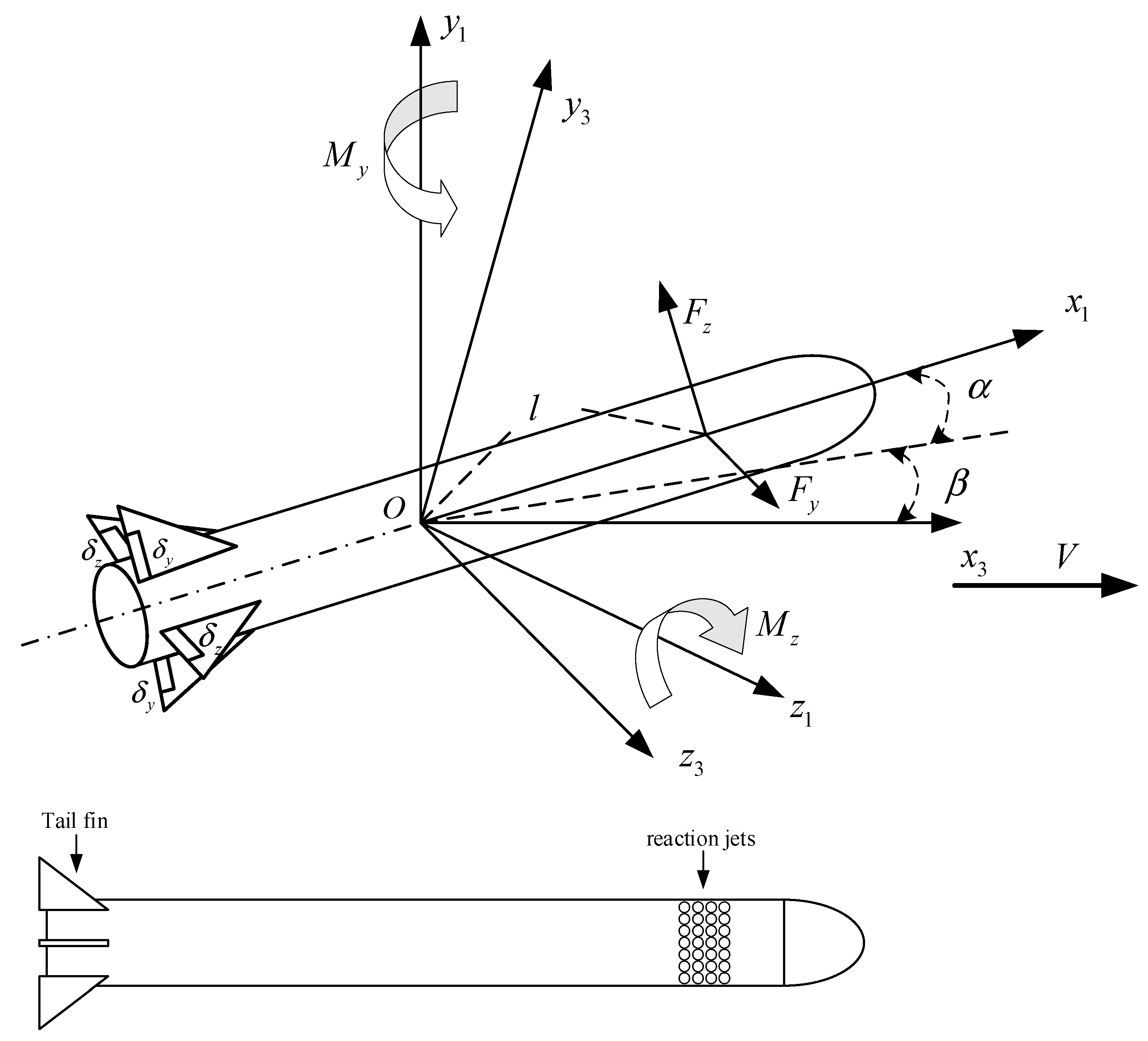
As shown in Figure 1, dual-control aircraft’s pitch and yaw channels have two control inputs, i.e., tail fins and reaction jets. Since the direct force is perpendicular to the axis of the aircraft, it will not affect the rolling channel, so there is only one control input in the roll channel, i.e., tail fins. Among them, the aircraft has four tail fins in a cross layout. Two vertical fins provide , two horizontal fins provide , and is generated by the differential between horizontal fins and vertical fins.
The missile body coordinate system and the missile velocity coordinate system are defined in Figure 1. The axis is the longitudinal axis of the missile and the axis is along , the velocity of the missile. The axis is in the plane of symmetry of the missile. The relationship between the two coordinate systems is determined by two angles, i.e., the angle of attack and the sideslip angle . Let denote the pitch rotational rate. We define the aerodynamic parameters in the elevation loop of the dual-control system as , , , , , , , , , , , , , , , , , .
Where is the partial derivative of the pitching moment with respect to the pitch rate , is the partial derivative of the pitching moment with respect to the angle of attack , is the partial derivative of the pitching moment with respect to the rudder deflection angle , is the partial derivative of the yaw moment with respect to the yaw rate , is the partial derivative of the yaw moment with respect to the sideslip angle , is the partial derivative of the yaw moment with respect to the rudder deflection angle , is the partial derivative of the roll moment with respect to the roll rate , is the partial derivative of the roll moment with respect to the rudder deflection angle , , and are the component of moment of inertia on axis , and respectively, and is the distance from the point of the lateral thrust to the mass center of the missile.
Considering entering the terminal guidance stage, the main engine of the aircraft is shut down, the aircraft mass and velocity are constant, and the attitude dynamics model of the dual-control aircraft is established through the above aerodynamic parameters.
The external forces on the missile are gravity, aerodynamic force, and direct force, so the missile overload dynamic model of the pitch channel can be written as
The derivative of Equation (6) is
By substituting Equations (1) and (3) into Equation (7), we can obtain
With further simplification, we obtain
The dynamic response of the controller actuator is considered as the inertial system, i.e.,
where and are the mechanical constants of the actuator, respectively.
By substituting Equation (6) into Equation (5), we obtain
Similarly, we can obtain the dynamic model of the yaw channel as
The attitude dynamics model of rolling channel considering three-channel coupling is
Finally, the aircraft attitude dynamics model is obtained as
We define as the state vector, where is the control vector, then Equation (18) can be written as the following state space model:
where
where is the external disturbance.
3. Design of Optimal Control Law Based on HJB Equation
Consider continuous affine nonlinear systems with a class of uncertainties
where is the state vector of the system, is the control input vector, and and are the system function and control matrix, respectively.
Assumption 1.
The nonlinear function satisfies the local Lipschitz condition in the set containing the origin and f(0) = 0. The control matrix is bounded.
Consider reference systems without uncertainties
Assumption 2.
There is a symmetric positive definite matrix such that the system uncertainty satisfies and the system uncertainty is bounded, that is, .
Based on the above assumptions, the control system cost function is defined as
where , is a symmetric positive definite matrix, and is defined as the tracking error.
Remark 1.
The minimum value of the cost function is achieved by searching for the optimal control term . When designing the cost function, the tracking error of the system and the upper bound of the uncertainty of the system are described, and it can be seen from the definition that 0. Therefore, when the minimum cost function is obtained, the closed-loop system state can converge to a sufficiently small neighborhood of the control command, and the interference of uncertainty is considered to achieve the effect of interference suppression.
According to the optimal control theory of nonlinear systems, the Hamiltonian function of the design reference system is
where is the partial derivative of the cost function with respect to the state of the system , i.e., .
The optimal cost function can be obtained by solving the following Hamilton–Jacobi–Bellman (HJB) Equation (24):
According to the necessary conditions 0, the optimal control law is
By substituting Equation (25) into Equation (24), the HJB equation can be rewritten as
Remark 2.
It can be seen that in order to obtain the optimal control law , the above HJB equation needs to be solved to obtain the optimal cost function and its partial derivative to the system state . However, for nonlinear systems, it is very difficult to solve the HJB equation, especially in the case of considering external disturbance, so the difficulty of solving the equation further increases. On the other hand, if we can find the cost function to ensure the Hamiltonian function , we can obtain the optimal control law . In other words, through this idea, the optimal control problem can be transformed into the problem of how to obtain the optimal cost function . In the next section, a reinforcement learning algorithm based on the LSTM neural network is proposed, which uses the LSTM neural network to fit the optimal cost function, so as to achieve approximate optimal control.
4. Design of Approximate Optimal Control Law Based on Reinforcement Learning
4.1. LSTM Neural Network
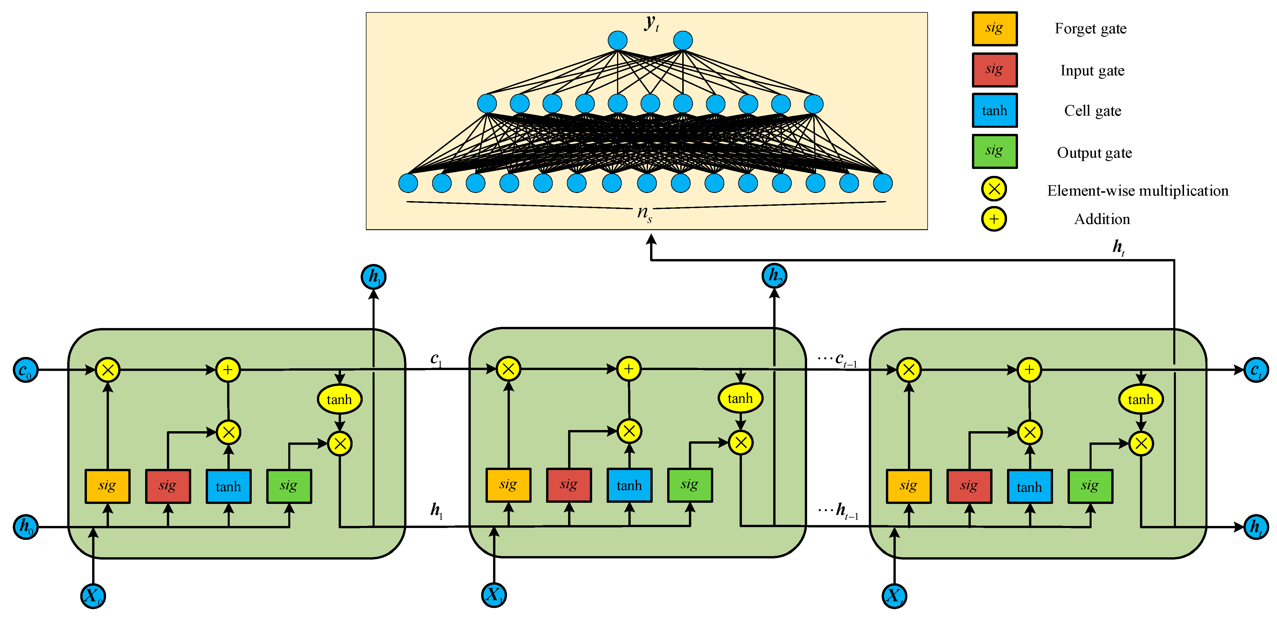
The LSTM neural network shown in Figure 2 contains three parts, i.e., a forget gate, an input gate, and an output gate. Except for the same hidden state as the RNNs, it also introduces a cell state for keeping the long-term memory information. At the current time t, the cell state is updated through the data from the forget gate and the input gate to achieve a long-term memory update. Then, the cell state , the last step hidden state , and the current step input are mixed via the output gate to obtain a network output. The details of the LSTM neural network can be obtained from another article [29]. The LSTM neural network is expressed as follows:
where denotes the element-wise multiplication; is the cell state vector; is the input vector; and , and are the input, forget, and output gates, respectively. The sigmoid function and the hyperbolic tangent function apply point-wise to the vector elements. Furthermore, , , , , , , , , , , , and are the weighting matrices.
According to Equation (36), we can know that the dimension of the output value of the LSTM neural network is related to the number of cell states. To obtain the output dimension we need, the usual method is introducing a scaling matrix , i.e., . However, when the scale difference between the input and output of the network is large, the value of each element in the scaling matrix will be too large or too small, which will affect the update of other weights of the network. Therefore, we introduce a full connection layer as the scaling matrix of the network to increase the depth of the network and improve the fitting accuracy of the network, i.e.,
4.2. Design of Near-Optimal Control Law Based on LSTM Neural Network and Output Feedback
The optimal output value of the neural network is defined as
Assumption 3.
There exist an optimal weight , standard bias terms , , , , and optimal network weights in approximating the unknown function which can be expressed as , where presents the optimal output value of , and is the mapping error uniformly bounded as , where is an arbitrarily small positive constant. The terms of the optimal weight matrices are all constant.
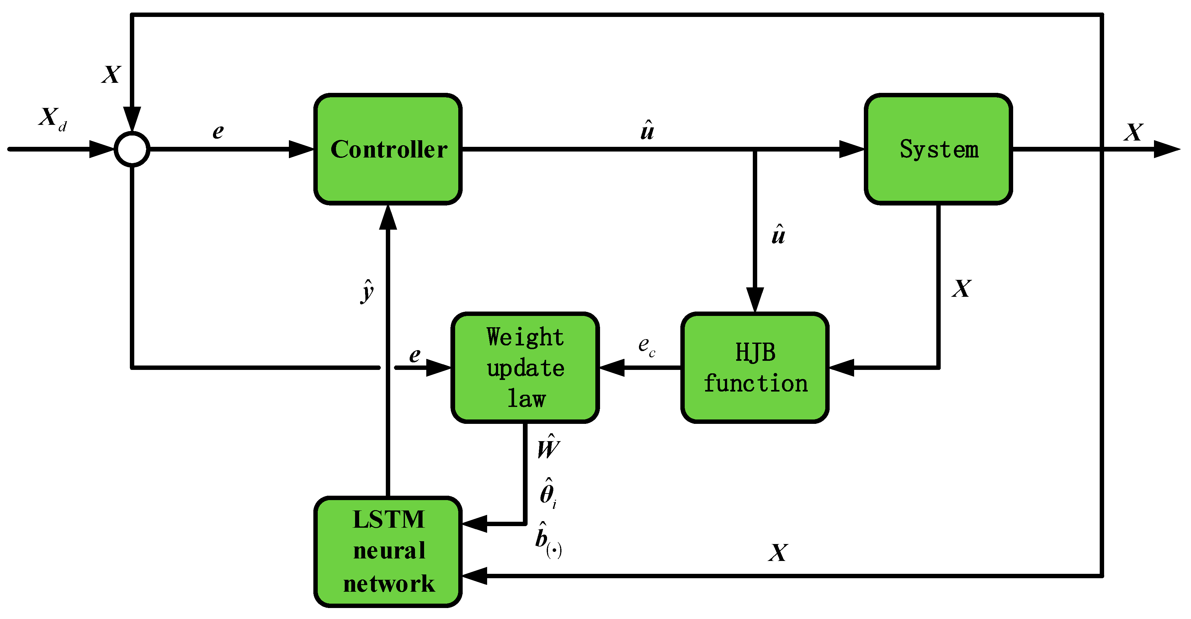
The detailed structure of the ADP-LSTM algorithm can be seen in Figure 3.
The difference between the estimated value and the optimal value of the Hamilton function is defined as the training error of the LSTM neural network, i.e.,
As we know from the last section, , and Equation (40) can be rewritten as
where is a positive definite matrix.
The difference between the neural network output and the optimal value is
where . By substituting Equation (42) into Equation (41), Equation (41) can be rewritten as
The time derivative of Equation (43) can be obtained as
where .
Theorem 1.
The following control law can ensure that the closed-loop system converges to a sufficiently small neighborhood of the control command, and the control law is approximately optimal.
where .
Remark 3.
The above control law is an improved form of the optimal control law (25) in the previous section, in which ensures that the system control input is approximately optimal. As an additional term, ensures that the tracking error of the closed-loop system finally converges to a sufficiently small neighborhood of the control command. The stability analysis will be given in the next section.
4.3. Design of Online Weight Update Law for LSTM Neural Networks
For brevity, we define , and by substituting it into the control law, we can obtain
According to the definition of and Assumption 3, we know that , so Equation (48) can be rewritten as
Also for brevity, we define and , where, by the difference method, we can obtain
Thus, Equation (49) can be further simplified as
Consider that is the output of the LSTM neural network, which can be expressed as
According to the Taylor expansion formula, we can obtain
where , .
Proof of Theorem 1.
To ensure that the tracking error of the Hamiltonian function can converge to 0, the Lyapunov function is defined as follows:
The time derivative of Equations (54) and (55) can be obtained as
To ensure that is negative, we set the
According to matrix operation rules, we can obtain
where is the i-th line of .
Expand the terms on the right side of Equation (58) to obtain
where , and are i-th elements of , and respectively.
By eliminating the corresponding term, the update law of the weight ’s i-th line is obtained as
Similarly, in order to obtain the update law of other weights, set
We can obtain
□
Remark 4.
By substituting the weight update law (63), (65)~(69), and the control law (45) into Equation (57), it can be obtained that . is a positive constant, so ; obviously, is positive, and according to the Lyapunov stability theory, closed-loop systems are bounded and . According to the optimal control theory, when , and ; at this point, the cost function is optimal. According to the definition of the cost function in Section 3, the system tracking error and control input are both considered; that is to say, the optimal performance cost function can ensure system tracking error 0, and the closed-loop control system is bounded and can converge to the small neighborhood of the control command.
Remark 5.
In this article, ADP-LSTM is described as a model-based reinforcement learning algorithm, rather than a data-based form. During the process of updating the weights of the LSTM neural networks, the algorithm does not rely on training data and loss functions, such as common stochastic gradient descent algorithms. Instead, it is based on the Lyapunov method, which directly provides an analytical solution for the network weight update law (63) and (65)~(69). In other words, ADP-LSTM does not require training data and loss functions. This direct update law eliminates a large number of iterative operations in the network training process, significantly reducing the system’s computational burden and single-step computation time.
5. Simulation Analysis
In the simulation process, the 6-DoF attitude dynamics model of the dual-control aircraft mentioned in the Section 2 is applied to verify the performance of the control law which is presented in this paper. The command signal is , and all aerodynamic parameters are designed based on an aircraft flying altitude of 30 km.
When the aircraft flies at an altitude of 30 km, the thin atmospheric density results in a decrease in aerodynamic force. At this time, relying on pure aerodynamic control will seriously reduce the dynamic characteristics and control quality of the control system. Usually, the dual-control strategy is used to design the aircraft autopilot, because the direct force is generated by the reaction jet, which is not affected by the flight altitude, and can effectively compensate for the lack of control input caused by insufficient aerodynamic force.
Due to the volume limitation of the aircraft, it is impossible to place the orbit control engine with a large volume and weight. Therefore, the attitude control engine is used in this simulation, which only affects the attitude and has a very small direct impact on the overload. Therefore, the overload establishment of the aircraft still depends on the aerodynamic force; that is to say, in order to obtain enough overload, the aircraft will make a large angle of attack or sideslip angle maneuver. At this time, the assumption that the aerodynamic parameters are considered as constant or slow time variables is no longer tenable. Therefore, taking the aerodynamic parameters and as examples, we consider and as functions of the AOA and sideslip angle, i.e.,
We consider other aerodynamic parameters as perturbation parameters, i.e.,
As the roll angle and roll rate are both small, we consider and as constants. We consider that the external disturbance vector is Gaussian white noise.
The initial weights of the LSTM neural network are randomly selected in the closed interval . According to the practical application, the tail fin angle and the magnitude of the direct force are subject to saturation constraints, i.e., , , , , and . The initial state of the system is .
To verify the optimality of ADP-LSTM, the adaptive sliding mode control method (SMC-RNN) proposed in reference [31] was applied to the attitude control model during the simulation process and compared with ADP-LSTM. The algorithm in reference [31] combines sliding mode control and Recurrent Neural Networks (RNN), using RNNs to fit system terms and external disturbances to achieve adaptive control of the system model and external disturbances. However, it is important to note that the algorithm in reference [31] did not consider energy optimization during its design process. Therefore, comparing it with ADP-LSTM can effectively reflect the energy-optimal control effect of ADP-LSTM.
The LSTM neural networks used in ADP-LSTM have eight input nodes, eight output nodes, and 10 cell states, making the system state the input vector of the network. The RNNs also have eight input nodes, eight output nodes, and 10 hidden states; the structure of RNNs can be found in the article [31].
To verify the control effectiveness of ADP-LSTM, two simulation scenarios are designed: tracking a fixed overload command and tracking a time-varying overload command. Both scenarios represent common target maneuver forms and can demonstrate the general applicability of the algorithm presented in this paper.
The aircraft parameters of the pitch channel can be seen in Table 1. Considering that the aircraft has an axisymmetric shape, the pitch channel parameters are consistent with the yaw channel parameters.
5.1. Scenario 1: Tracking a Fixed Overload Command
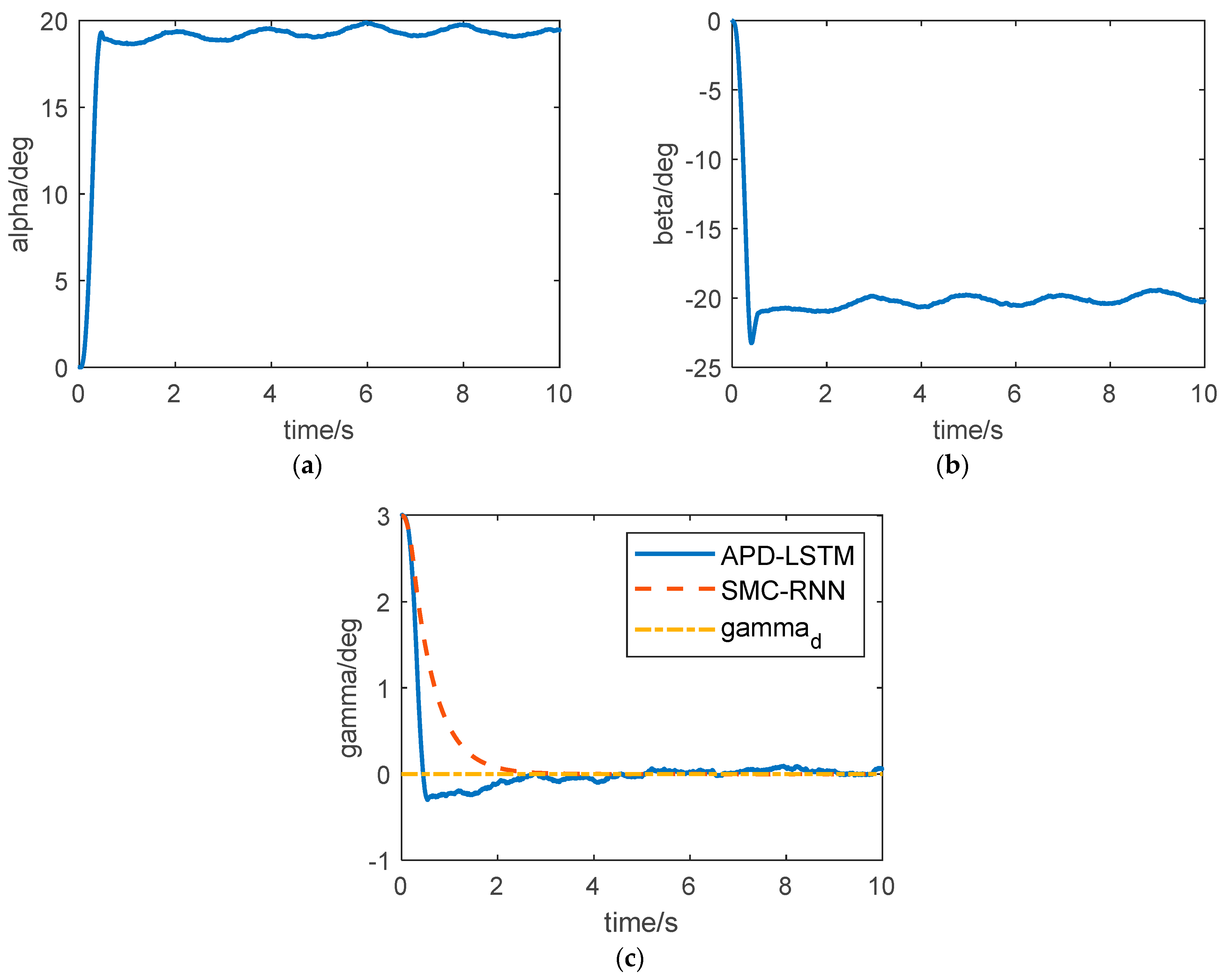
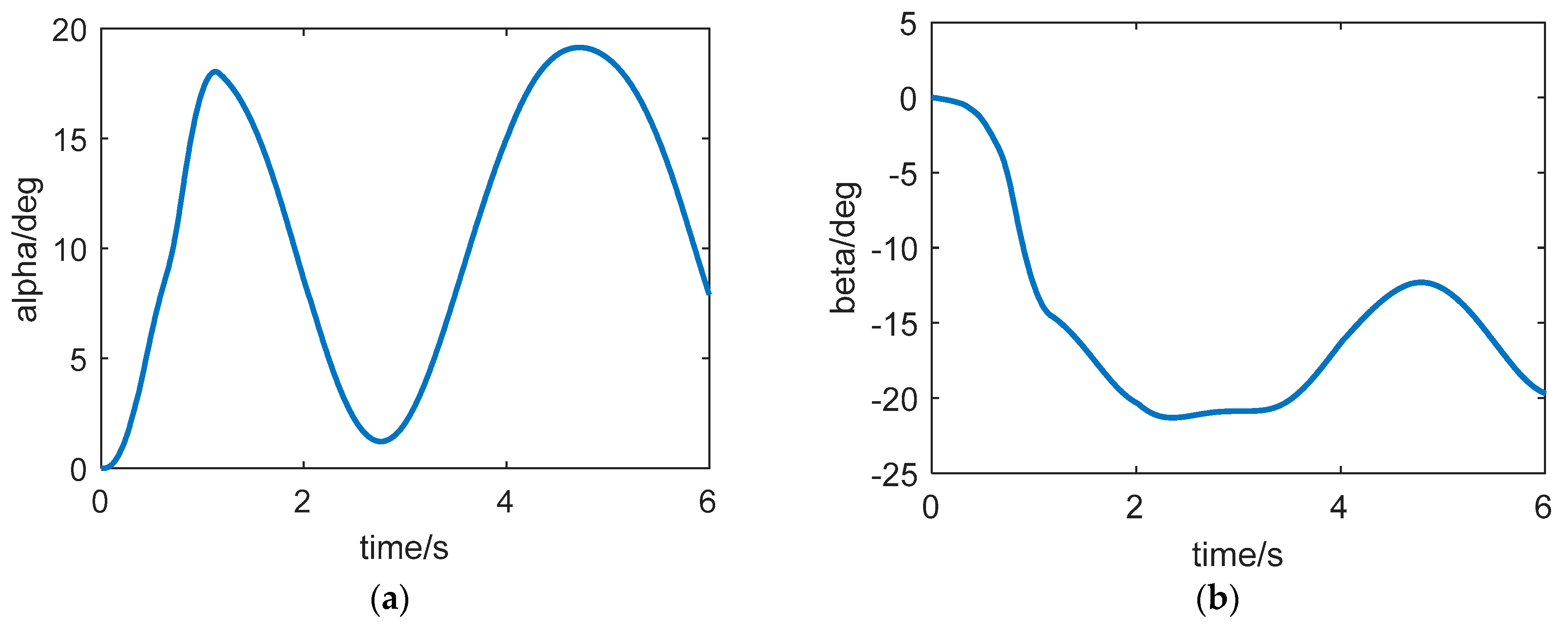
The curve of the angle of attack, sideslip angle, and roll angle are shown in Figure 4. According to the previous introduction, the overload of the aircraft is established by the aerodynamic force, so in order to track the overload command as soon as possible, the angle of attack and sideslip angle of the aircraft need to respond quickly. In Figure 4a,b, we can see that the angle of attack and sideslip angle both enter the steady state quickly. Like other STT aircraft, the controller designed in this paper ensures that the aircraft body axis does not roll; that is, the roll angle command is 0 deg. To verify the effect of the controller, the initial roll angle is set to 3 degrees. As can be seen from Figure 4c, the controller can ensure that the roll angle converges to 0 deg. Both ADP-LSTM and SMC-RNN can achieve control of roll angle, among which ADP-LSTM has a faster convergence speed but some overshoot, while SCM-RNN, although it has no overshoot, has a slower convergence speed.
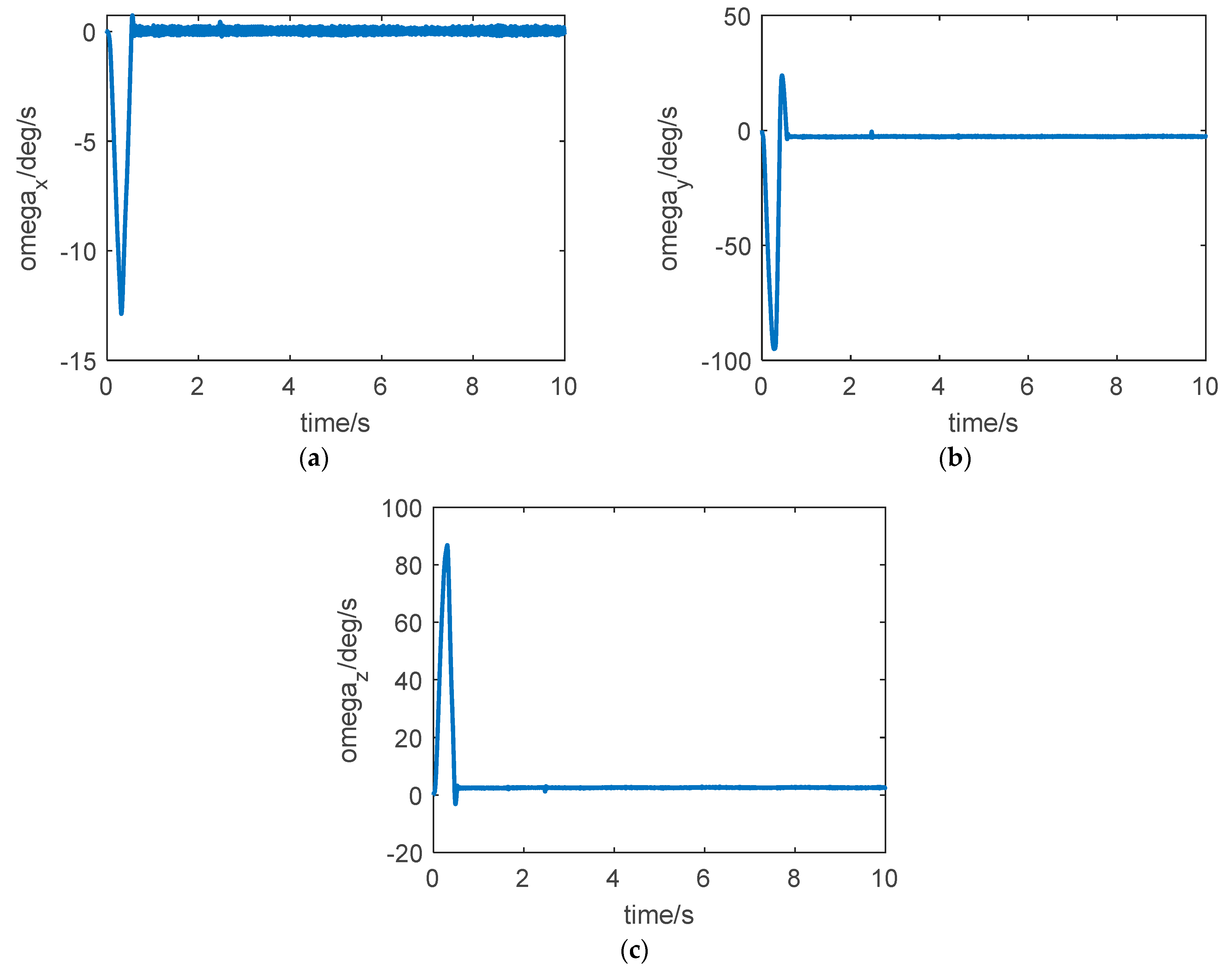
The curve of roll rate, yaw rate, and pitch rate are shown in Figure 5. This state intuitively reflects the attitude agility of the aircraft. It can be seen from Figure 5 that the aircraft has strong agility and fast attitude response speed under the effect of the dual-control strategy.
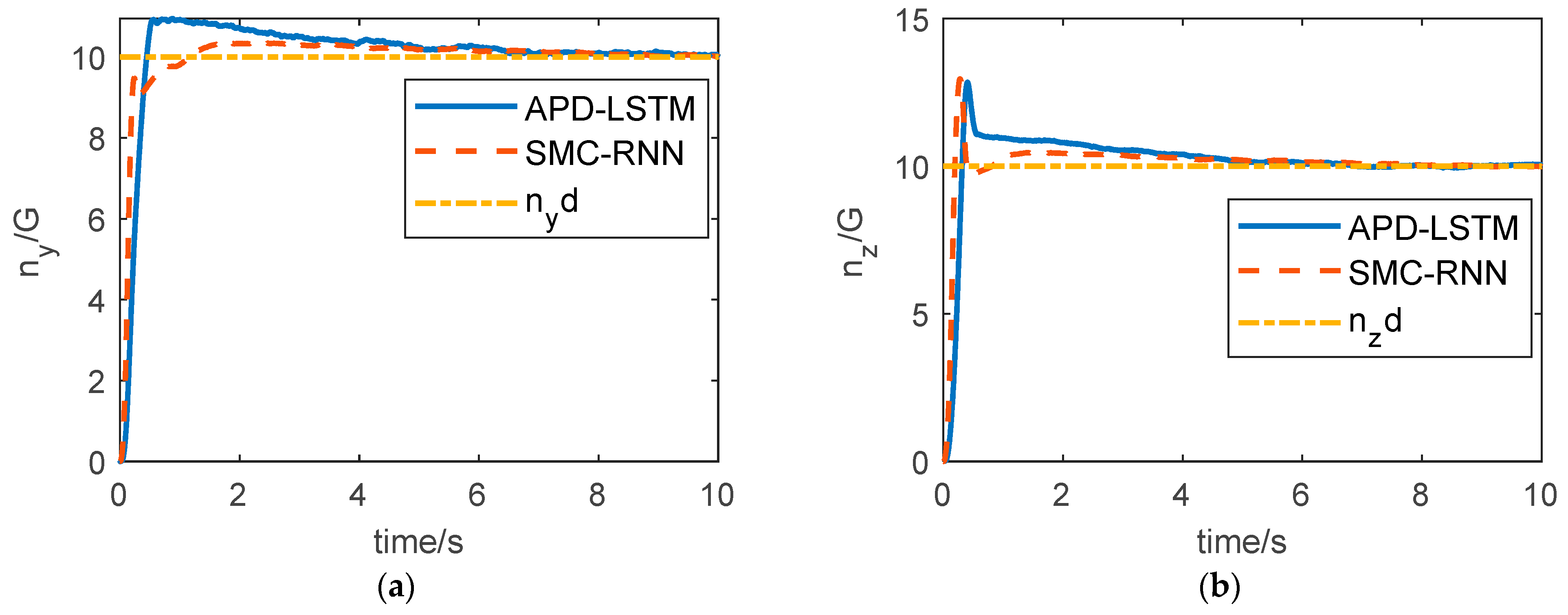
The overload curves of the two controllers are shown in Figure 6. It can be seen from Figure 6 that the aircraft overload can track the command signal by ADP-LSTM, but it has to be admitted that the convergence rate is slow for two reasons. First, according to the nonlinear system optimal control theory, when the Hamilton function tends to zero, the optimal control input obtained at this time can only ensure that the tracking error converges to 0 in infinite time, i.e., 0. Second, there are coupling terms between the pitch, yaw, and roll channels of the aircraft, which reduce the control quality. Usually, when designing the autopilot, it is completed after decoupling the three channels. However, this will ignore some characteristics of the system, and obviously, this will reduce the robustness of the algorithm in practical applications. The advantage of the ADP-LSTM in this paper is that it does not need three-channel decoupling, retains the characteristics of the system, and does not need the necessary assumptions when decoupling, which widens the application scope of the algorithm and is more general. Meanwhile, we can observe that the control effect of SMC-RNN is better than that of ADP-LSTM. This is an unavoidable trade-off. In order to achieve optimal energy consumption for the system, some sacrifice in control effectiveness is inevitable. However, the control effectiveness of ADP-LSTM has not significantly decreased and still maintains steady-state error, with only a slight increase in convergence time.
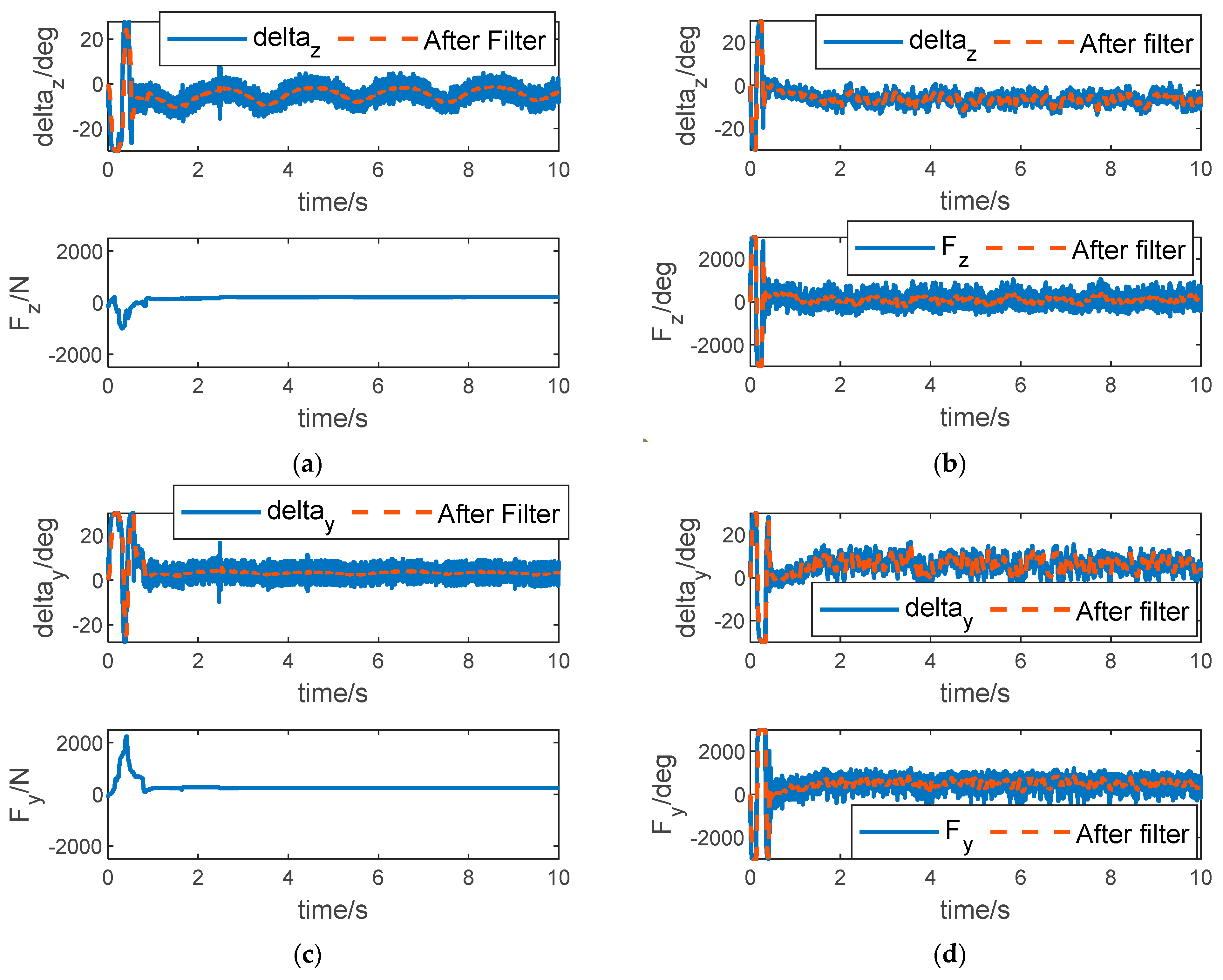
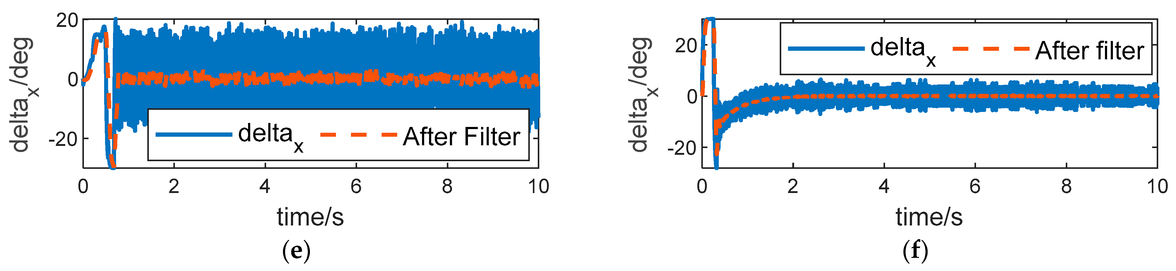
The control inputs of pitch, yaw, and roll channels of ADP-LSTM and SMC-RNN are shown in Figure 7. And low-pass filters were introduced to better display the specific details of the curve. It can be seen from Figure 7a,c,e that when the system enters the steady state, the control input of the tail fins has a chattering phenomenon, which is caused by external disturbance, and the control input shows a sinusoidal trend, which is caused by the perturbation of aerodynamic parameters. The direct force input will tend to a fixed value, and this value is very small. Intuitively, this avoids the waste of control energy. However, it is still impossible to determine whether the control input is optimal from the results of this figure alone. It is necessary to refer to whether the Hamiltonian function converges to zero. In Figure 7b,d,f, we can see that the control input of SMC-RNN is higher than that of ADP-LSTM, especially for direct force control input. The chattering phenomenon in the control input is more severe, and it does not significantly weaken after passing through the low-pass filter. This is due to the inherent defect of sliding mode control. Controlling the input chattering phenomenon can cause serious energy waste, and it is also very unfriendly to the actuator.
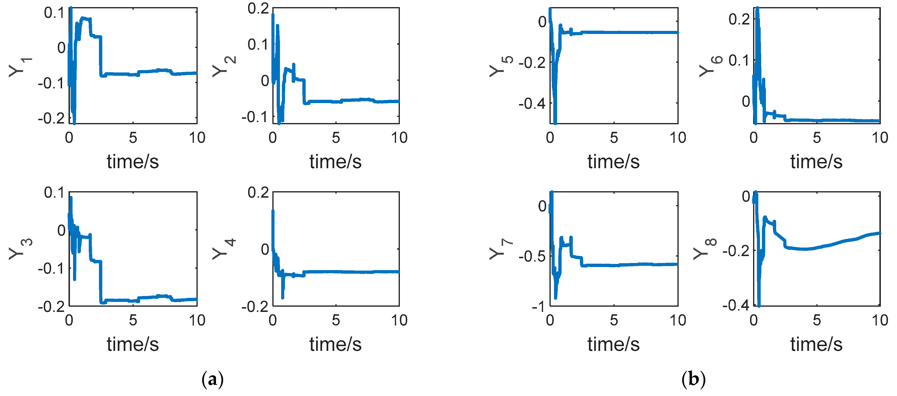
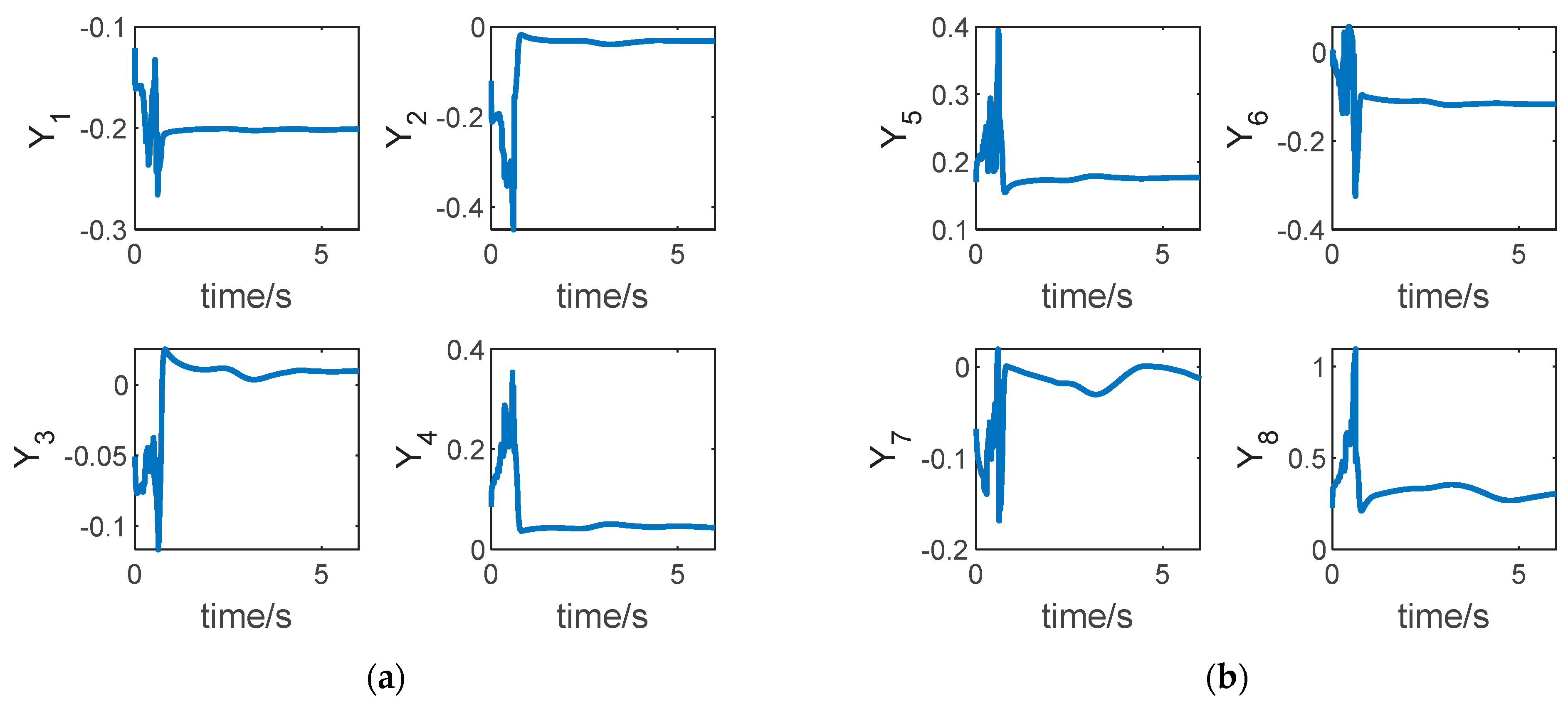
The outputs of the LSTM neural network are shown in Figure 8. In this paper, the LSTM neural network is aimed to fit the partial derivative of the cost function with respect to the state of the system , i.e., . According to the definition of the system, we know that , and there are eight output values of the LSTM neural network, i.e., . It can be seen from Figure 7 that after a short dynamic process, the output value of the neural network is nearly stable, which shows that under the effect of the adaptive weight update law, the output value gradually tends to the optimal value .
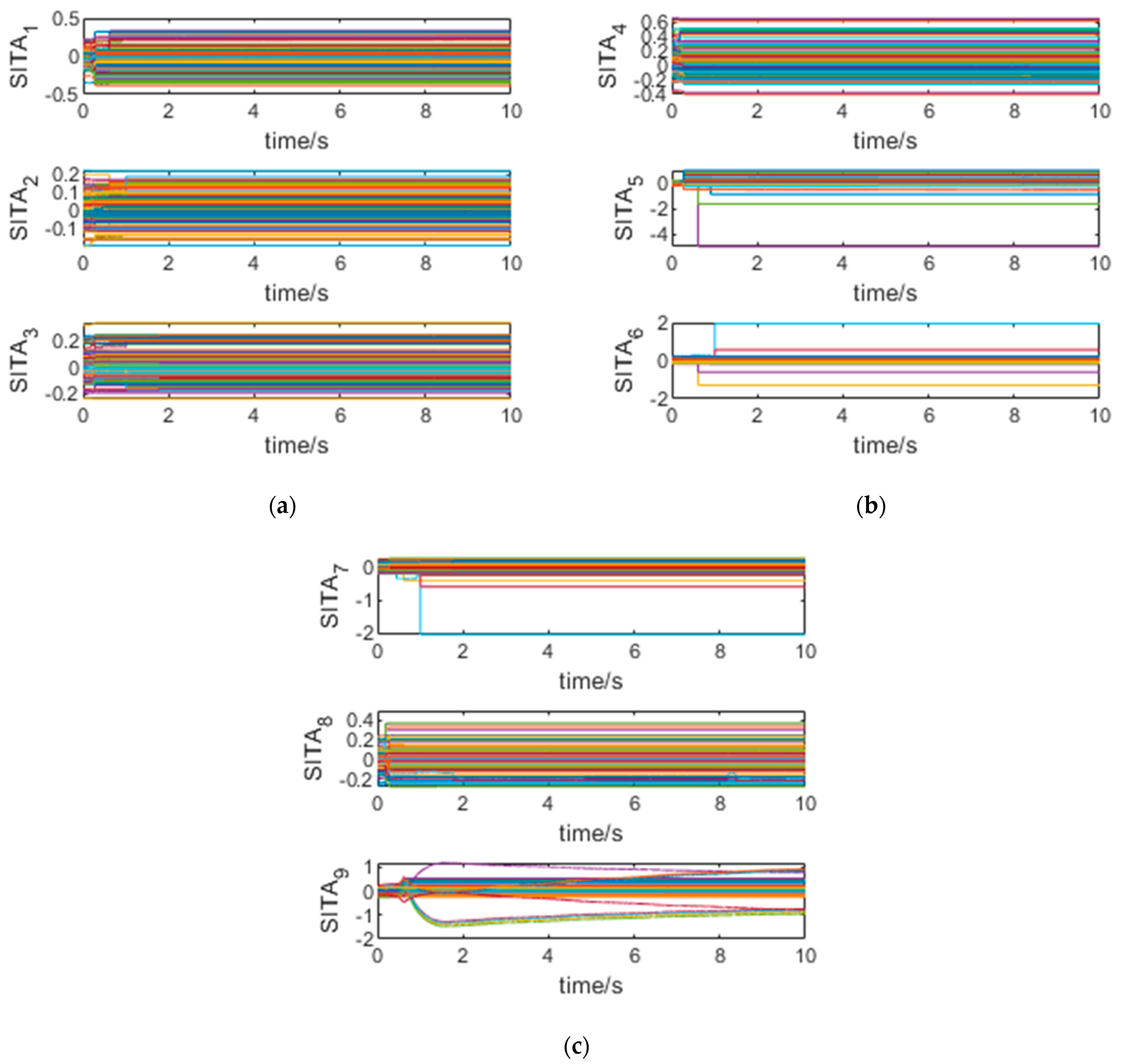
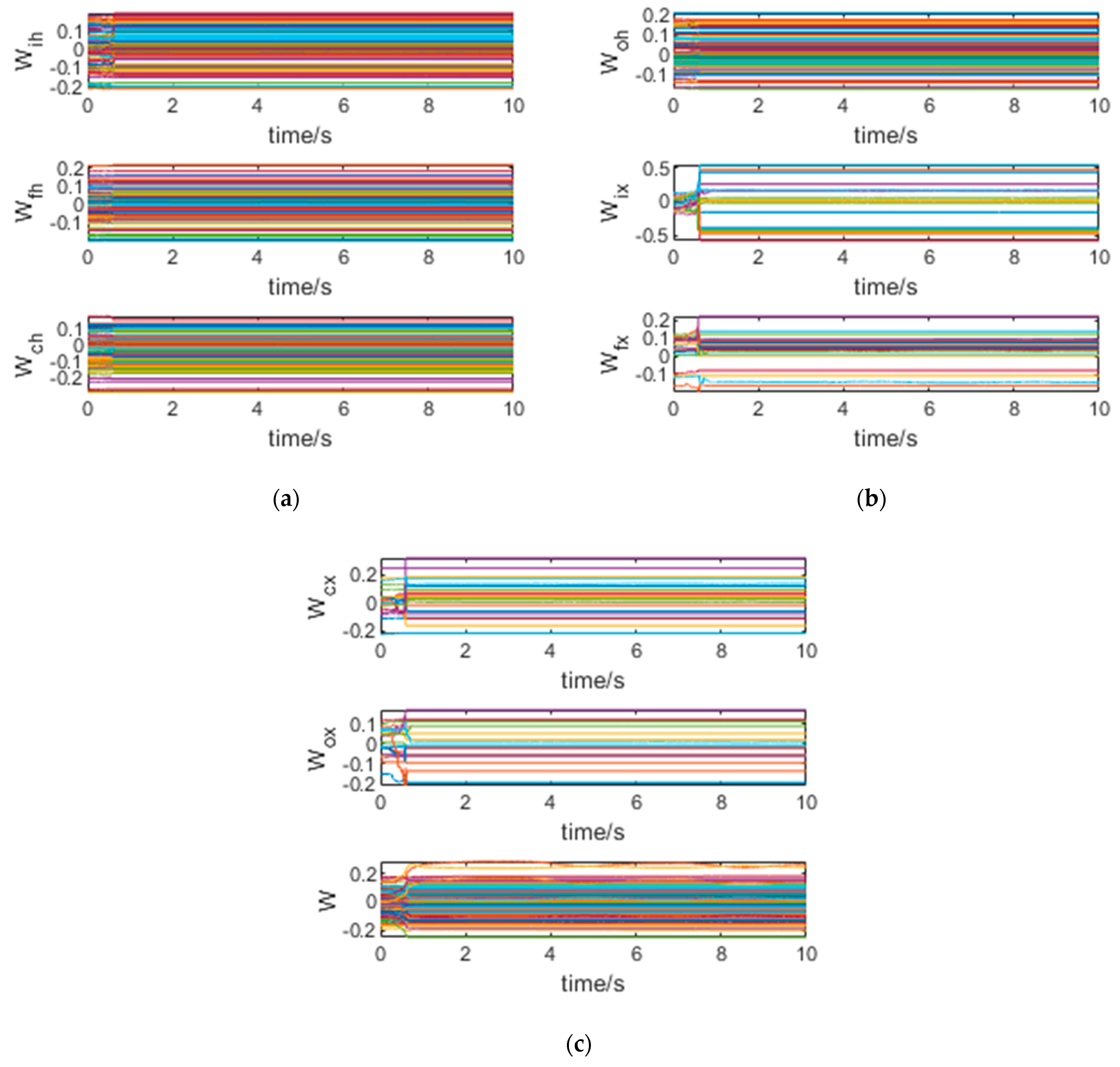
The training process is shown in Figure 9. It can be seen from the figure that under the effect of the adaptive weight update law, most neural network weights converge in 1 s, which shows that the training efficiency is very high. Because the updated law of network weights is derived from the Lyapunov function, the training trend of network weights is very clear, which must have obvious advantages over the stochastic gradient descent (SDG) method, and there are no problems such as local optimization in the training process.
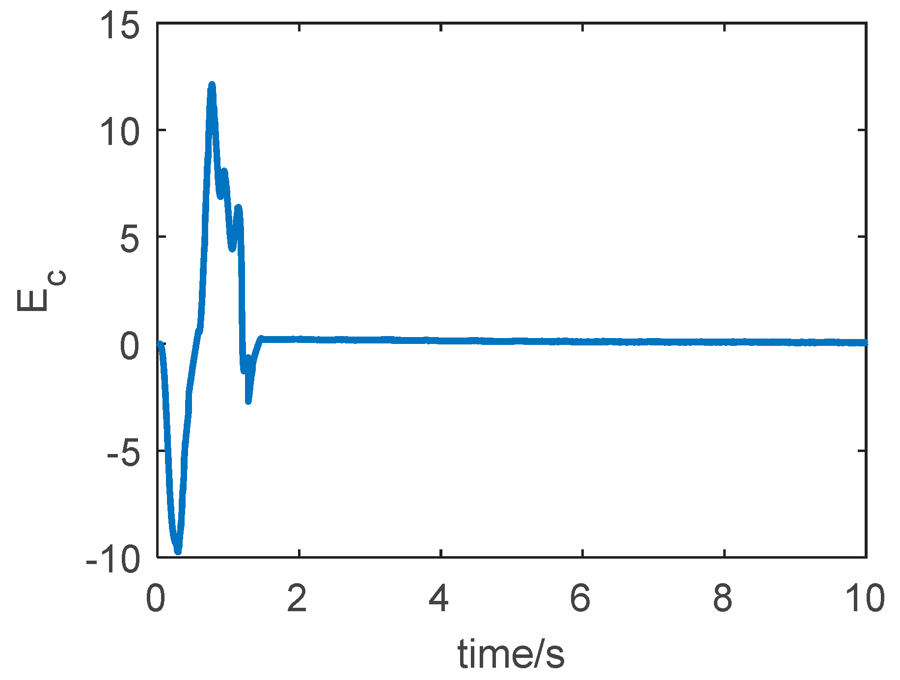
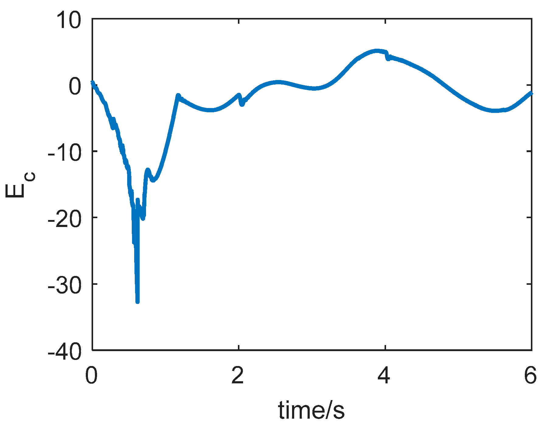
The curve of the Hamiltonian function is shown in Figure 10. According to the nonlinear system optimal theory mentioned in Section 3, the necessary condition for the optimal control input is that the Hamiltonian function tends to zero, i.e., and then It can be seen from the figure that under the action of the LSTM neural network, the Hamiltonian function converges to 0 quickly, indicating that and , and at this time, .
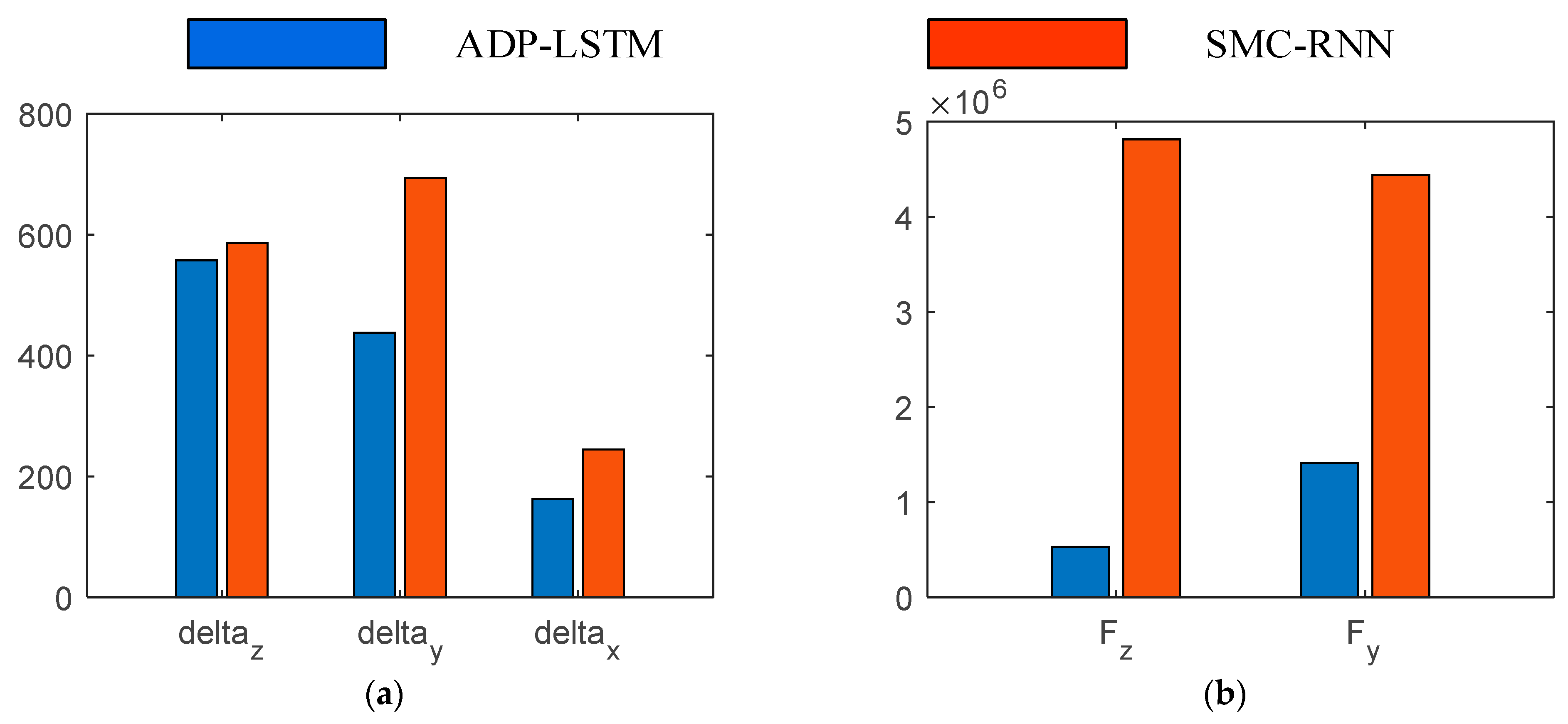
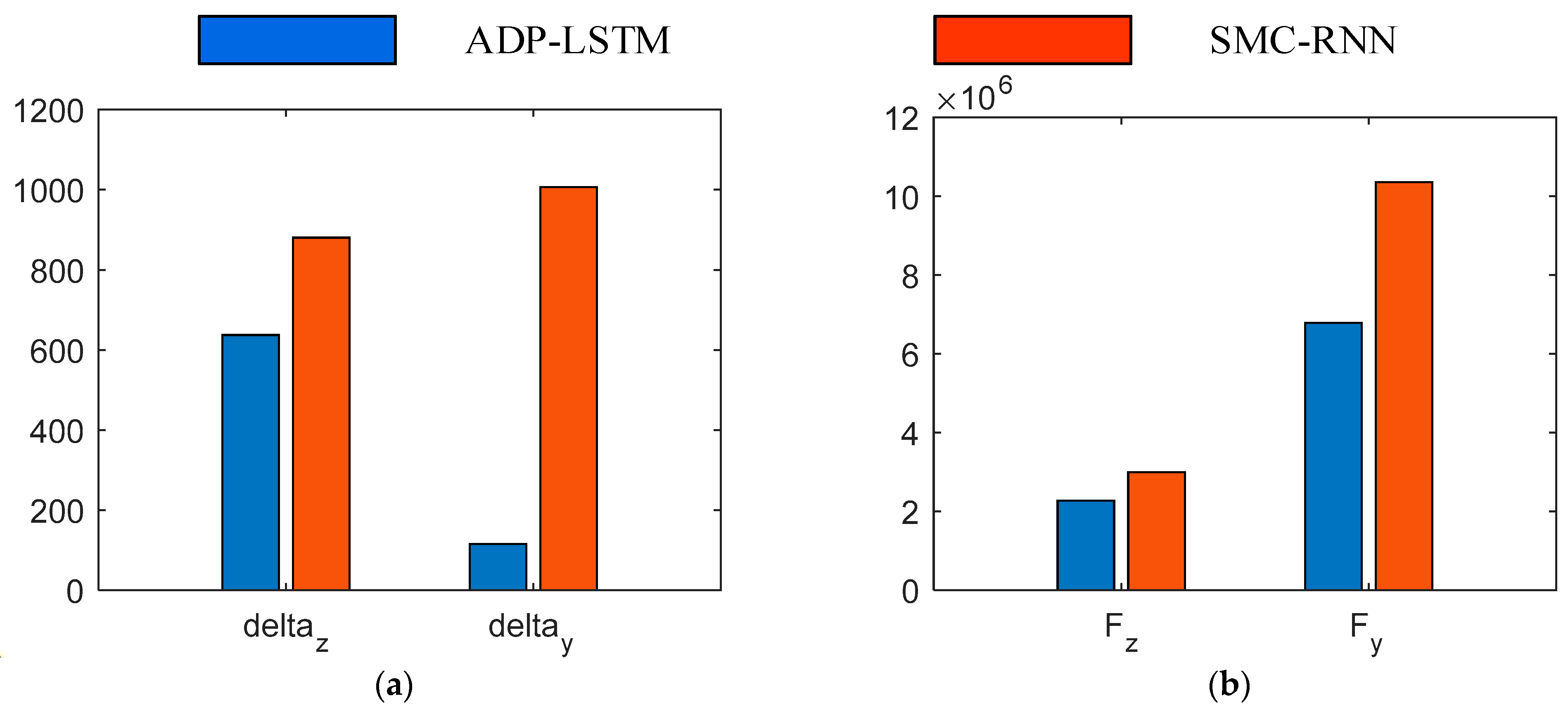
The energy consumption of the two control algorithms is shown in Figure 11. To quantify energy consumption, the energy consumption indicator is defined as . Figure 7a illustrates the energy consumption of the tail fins, while Figure 7b shows the energy consumption of the direct force. It is important to note that the values after low-pass filtering were used when calculating energy consumption. From Figure 7, it is evident that the energy consumption of both the tail fins and direct force using ADP-LSTM is superior to that of SMC-RNN. Particularly in the case of direct force energy consumption, ADP-LSTM demonstrates clear advantages, effectively avoiding energy waste. While ADP-LSTM may be slightly inferior to SMC-RNN in terms of control effectiveness, it holds significant advantages in energy consumption. As previously introduced, the energy of direct force is limited, and the aircraft will encounter multiple attitude adjustments and overload command tracking in a complete working environment. Without limiting energy consumption, early depletion of aircraft fuel can occur, leading to a loss of partial tracking ability. Therefore, this article focuses on studying the optimal control of aircraft attitude.
The average single-step time of the two algorithms is ADP-LSTM 1.105 ms, and SMC-RNN 0.751 ms (simulation environment: Intel 12th i7-12700).
5.2. Scenario 2: Tracking a Time-Varying Overload Command
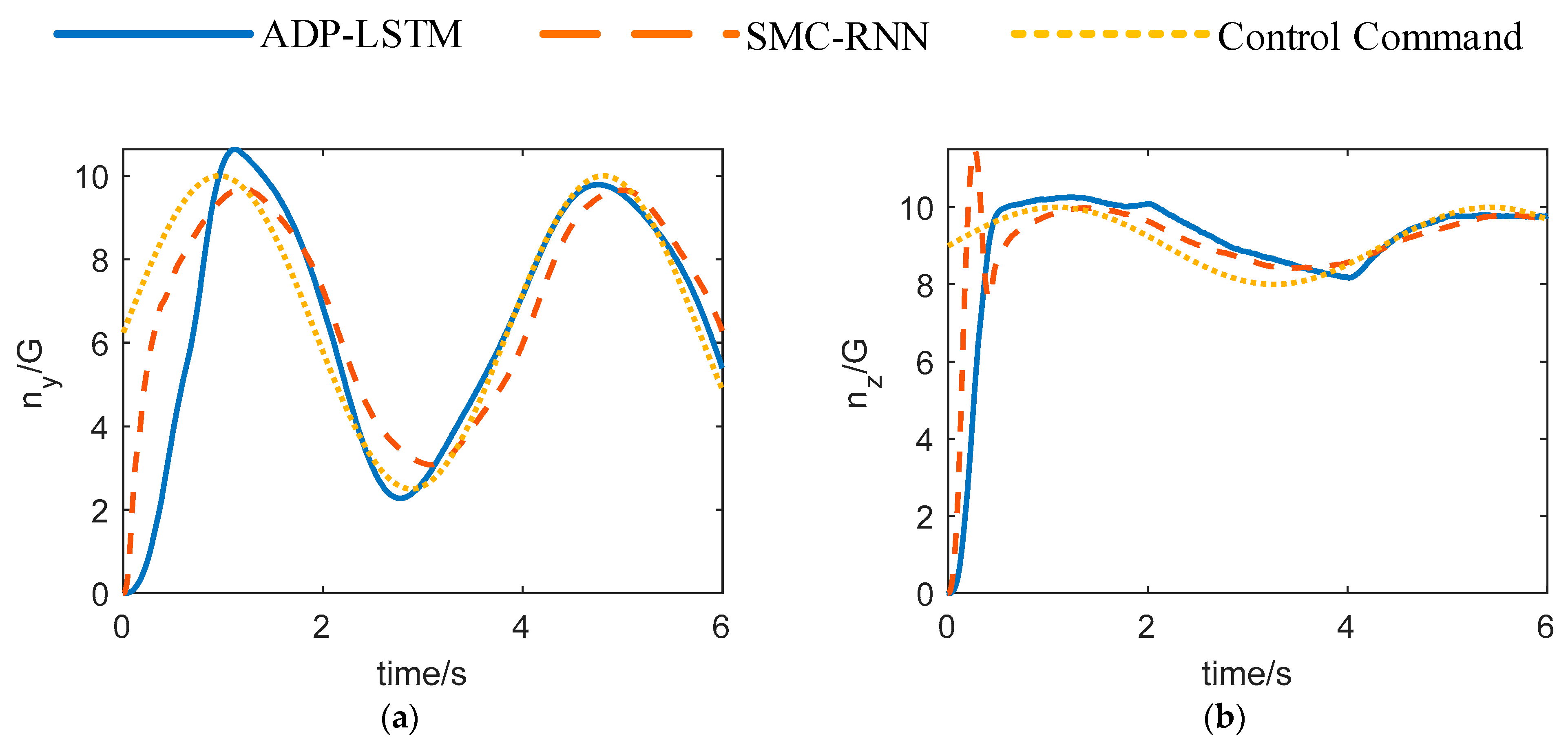
The simulation results for Scenario 2 are shown in Figure 12, Figure 13, Figure 14, Figure 15, Figure 16, Figure 17, Figure 18 and Figure 19. Similar to Scenario 1, both ADP-LSTM and SMC-RNN can track time-varying overload commands. However, the control effectiveness of ADP-LSTM is slightly weaker than that of SMC-RNN. This can be attributed to two reasons: 1. The convergence speed of the LSTM neural network is slightly slower than that of a traditional RNN, especially under time-varying commands, which becomes more apparent. 2. To achieve energy-optimal control, it is necessary to sacrifice some control effectiveness, especially in terms of command tracking speed. From Figure 14, it can be observed that although ADP-LSTM has a slightly slower convergence speed than SMC-RNN, there is no significant difference in their tracking accuracy, which is consistent with the performance in Scenario 1.
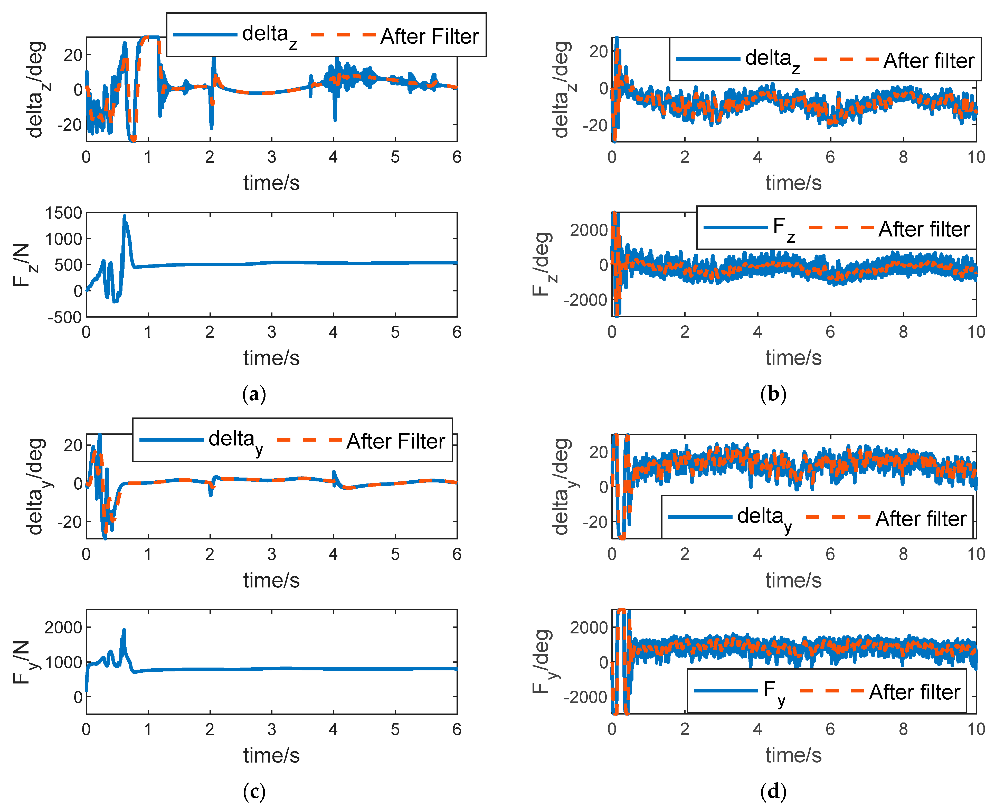
Figure 15 illustrates the control inputs of the two control algorithms. It is evident from the figure that SMC-RNN’s control input exhibits significant oscillations, similar to Scenario 1. This is unfriendly to the control execution mechanism and results in a significant waste of energy. In contrast, ADP-LSTM does not exhibit such oscillations. Furthermore, from Figure 19, it can be seen that the energy consumption of ADP-LSTM is significantly lower than that of SMC-RNN (after the filtering of SMC-RNN’s control input). This demonstrates the significant advantage of ADP-LSTM in energy-optimal control.
Through the above two simulation scenarios, it is evident that ADP-LSTM can handle common aircraft overload commands and has a certain degree of generality.
6. Conclusions
This article presents a reinforcement learning near-optimal control algorithm based on an LSTM neural network, which can be applied to solve the 6-DoF attitude control problem of dual-control aircraft. For the first time, the reinforcement learning-based near-optimal control algorithm is applied to the complex MIMO system.
Compared with the existing reinforcement learning algorithm, this algorithm has an obvious advantage:
- (1)
- It can deal with high-dimensional MIMO systems, rather than ideal simple systems such as inverted pendulum, slider car, spring damper, and other SIMO or SISO systems, which benefit from the strong fitting ability of LSTM neural network;
- (2)
- The ADP-LSTM does not need to decouple the nonlinear aircraft 6-DoF attitude dynamics model, and it retains the internal characteristics of the system as much as possible and the assumptions of necessity when system decoupling is no longer needed, making the algorithm more universal.
- (3)
- Based on the Lyapunov method, the novel adaptive online update law of LSTM neural network weights is given. Compared with the stochastic gradient descent method, this method has higher training efficiency and can ensure that the closed-loop system is uniformly asymptotically stable.
- (4)
- During the simulation process, we designed two kinds of scenarios to prove the commonality of ADP-LSTM, which was compared with SMC-RNN in terms of control effectiveness and energy consumption. The comparison results revealed that ADP-LSTM had a significant advantage in energy consumption, albeit at the expense of sacrificing some control effectiveness. This reflects the overall advantage of ADP-LSTM over algorithms that do not consider energy optimization.
As for the future research direction, I think the main direction in the near future is how to solve the optimal control problem when the control input is saturated, and a longer-term goal is how to realize the finite-time convergence of the system.
Author Contributions
Conceptualization, Y.Y. and D.Z.; methodology, Y.Y.; software, Y.Y.; validation, Y.Y.; formal analysis, Y.Y.; investigation, D.Z.; resources, D.Z.; data curation, Y.Y.; writing—original draft preparation, Y.Y.; writing—review and editing, D.Z.; visualization, Y.Y.; supervision, D.Z.; project administration, D.Z.; funding acquisition, D.Z. All authors have read and agreed to the published version of the manuscript.
Funding
This research received no external funding.
Data Availability Statement
The data presented in this study are available on request from the corresponding author due to privacy issues.
Conflicts of Interest
The authors declare no conflicts of interest.
Abbreviations
| Angle of attack | |
| Sideslip angle | |
| Roll angle | |
| Moment of inertia about the ox1 axis | |
| Moment of inertia about the oy1 axis | |
| Moment of inertia about the oz1 axis | |
| Roll rate | |
| Yaw rate | |
| Pitch rate | |
| Rolling moment | |
| Yaw moment | |
| Pitch moment | |
| Projection of overload vector on oy1 axis | |
| Projection of overload vector on oz1 axis | |
| Rudder deflection angle of rolling channel | |
| Rudder deflection angle of yaw channel | |
| Rudder deflection angle of pitch channel | |
| Projection of direct force on oy1 axis | |
| Projection of direct force on oz1 axis | |
| Distance from the point of the lateral thrust to the mass center of the aircraft | |
| Aircraft mass | |
| Aircraft speed | |
| Gravitational acceleration | |
| Lift | |
| Lateral force |
References
- Kim, S.; Cho, D.; Kim, H.J. Force and moment blending control for fast response of agile dual missiles. IEEE Trans. Aerosp. Electron. Syst. 2016, 52, 938–947. [Google Scholar] [CrossRef]
- Tournes, C.; Shtessel, Y.; Shkolnikov, I. Autopilot for missiles steered by aerodynamic lift and divert thrusters using nonlinear dynamic sliding manifolds. In AIAA Guidance, Navigation, and Control Conference and Exhibit; AIAA: San Francisco, CA, USA, 2005. [Google Scholar]
- Shtessel, Y.; Tournes, C.; Shkolnikov, I. Guidance and autopilot for missiles steered by aerodynamic lift and divert thruster using second order sliding modes. In AIAA Guidance, Navigation, and Control Conference and Exhibit; AIAA: Keystone, CO, USA, 2006. [Google Scholar]
- Hirokawa, R.; Sato, K.; Manabe, S. Autopilot design for a missile with reaction-jet using coefficient diagram method. In AIAA Guidance, Navigation, and Control Conference and Exhibit; AIAA: Montreal, QC, Canada, 2001. [Google Scholar]
- Thukral, A.; Innocenti, M. A sliding mode missile pitch autopilot synthesis for high angle of attack maneuvering. IEEE Trans. Control. Syst. Technol. 1998, 6, 359–371. [Google Scholar] [CrossRef]
- Yeh, F.-K.; Cheng, K.-Y.; Fu, L.-C. Variable structure-based nonlinear missile guidance/autopilot design with highly maneuverable actuators. IEEE Trans. Control. Syst. Technol. 2004, 12, 944–949. [Google Scholar]
- Werbos, P. Beyond Regression: New Tools for Prediction and Analysis in the Behavioral Sciences. Ph.D. Thesis, Harvard University, Cambridge, MA, USA, 1974. [Google Scholar]
- Wang, T.; Wang, Y.; Yang, X.; Yang, J. Further Results on Optimal Tracking Control for Nonlinear Systems with Nonzero Equilibrium via Adaptive Dynamic Programming. IEEE Trans. Neural Netw. Learn. Syst. 2023, 34, 1900–1910. [Google Scholar] [CrossRef] [PubMed]
- Liu, D.; Wei, Q. Policy Iteration Adaptive Dynamic Programming Algorithm for Discrete-Time Nonlinear Systems. IEEE Trans. Neural Netw. Learn. Syst. 2014, 25, 621–634. [Google Scholar] [CrossRef] [PubMed]
- Bian, T.; Jiang, Z.-P. Reinforcement Learning and Adaptive Optimal Control for Continuous-Time Nonlinear Systems: A Value Iteration Approach. IEEE Trans. Neural Netw. Learn. Syst. 2022, 33, 2781–2790. [Google Scholar] [CrossRef] [PubMed]
- Gao, W.; Jiang, Z.-P. Adaptive Dynamic Programming and Adaptive Optimal Output Regulation of Linear Systems. IEEE Trans. Autom. Control. 2016, 61, 4164–4169. [Google Scholar] [CrossRef]
- Jiang, Y.; Jiang, Z.-P. Global Adaptive Dynamic Programming for Continuous-Time Nonlinear Systems. IEEE Trans. Autom. Control. 2015, 60, 2917–2929. [Google Scholar] [CrossRef]
- Bo, P.; Jiang, Z.-P.; Mareels, I. Reinforcement learning for adaptive optimal control of continuous-time linear periodic systems. Automatica 2020, 118, 109035. [Google Scholar]
- Asad Rizvi, S.A.; Lin, Z. Output feedback adaptive dynamic programming for linear differential zero-sum games. Automatica 2020, 122, 109272. [Google Scholar] [CrossRef]
- Xie, K.; Yu, X.; Lan, W. Optimal output regulation for unknown continuous-time linear systems by internal model and adaptive dynamic programming. Automatica 2022, 146, 110564. [Google Scholar] [CrossRef]
- Jia, S.; Tang, Y.; Wang, T.; Ding, Q. A novel active control on Pogo vibration in liquid rockets based on data-driven theory. Acta Astronaut. 2021, 182, 350–360. [Google Scholar] [CrossRef]
- Nie, W.; Li, H.; Zhang, R. Model-free adaptive optimal design for trajectory tracking control of rocket-powered vehicle. Chin. J. Aeronaut. 2020, 33, 1703–1716. [Google Scholar] [CrossRef]
- Xue, S.; Luo, B.; Liu, D. Integral reinforcement learning based event-triggered control with input saturation. Neural Netw. 2020, 131, 144–153. [Google Scholar] [CrossRef] [PubMed]
- Long, T.; Cao, Y.; Sun, J.; Xu, G. Adaptive event-triggered distributed optimal guidance design via adaptive dynamic programming. Chin. J. Aeronaut. 2022, 35, 113–127. [Google Scholar] [CrossRef]
- Yang, B.; Jing, W.; Gao, C. Online midcourse guidance method for boost phase interception via adaptive convex programming. Aerosp. Sci. Technol. 2021, 118, 107037. [Google Scholar] [CrossRef]
- Han, X.; Zheng, Z.; Liu, L.; Wang, B.; Cheng, Z.; Fan, H.; Wang, Y. Online policy iteration ADP-based attitude-tracking control for hypersonic vehicles. Aerosp. Sci. Technol. 2020, 106, 106233. [Google Scholar] [CrossRef]
- Xiao, N.; Xiao, Y.; Ye, D.; Sun, Z. Adaptive differential game for modular reconfigurable satellites based on neural network observer. Aerosp. Sci. Technol. 2022, 128, 107759. [Google Scholar] [CrossRef]
- Tian, D.; Guo, J.; Guo, Z. Multi-objective optimization of actuators and consensus ADP-based vibration control for the large flexible space structures. Aerosp. Sci. Technol. 2023, 137, 108280. [Google Scholar] [CrossRef]
- Guo, Y.; Chen, G.; Zhao, T. Learning-based collision-free coordination for a team of uncertain quadrotor UAVs. Aerosp. Sci. Technol. 2021, 119, 107127. [Google Scholar] [CrossRef]
- Wang, Q.; Gong, L.; Dong, C.; Zhong, K. Morphing aircraft control based on switched nonlinear systems and adaptive dynamic programming. Aerosp. Sci. Technol. 2019, 93, 105325. [Google Scholar] [CrossRef]
- Mu, C.; Ni, Z.; Sun, C.; He, H. Air-Breathing Hypersonic Vehicle Tracking Control Based on Adaptive Dynamic Programming. IEEE Trans. Neural Netw. Learn. Syst. 2017, 28, 584–598. [Google Scholar] [CrossRef] [PubMed]
- Zhang, H.; Wang, H.; Niu, B.; Zhang, L.; Adil, M. Ahmad, Sliding-mode surface-based adaptive actor-critic optimal control for switched nonlinear systems with average dwell time. Inf. Sci. 2021, 580, 756–774. [Google Scholar] [CrossRef]
- Bengio, Y.; Simard, P.; Frasconi, P. Learning long-term dependencies with gradient descent is difficult. IEEE Trans. Neural Netw. 1994, 5, 157–166. [Google Scholar] [CrossRef] [PubMed]
- Hochreiter, S.; Schmidhuber, J. Long short-term memory. Neural Comput. 1997, 9, 1735–1780. [Google Scholar] [CrossRef] [PubMed]
- Smith, A.W.; Zipser, D. Learning sequential structure with the real time recurrent learning algorithm. Int. J. Neural. Syst. 1989, 1, 125–131. [Google Scholar] [CrossRef]
- Chu, Y.; Fei, J.; Hou, S. Dynamic global proportional integral derivative sliding mode control using radial basis function neural compensator for three-phase active power filter. Trans. Inst. Meas. Control. 2018, 40, 3549–3559. [Google Scholar] [CrossRef]
Figure 1.
Dual-control aircraft.

Figure 2.
LSTM neural network structure.

Figure 3.
The structure of the ADP-LSTM algorithm.

Figure 4.
Steady-state responses of angle of attack, sideslip angle, and roll angle in Scenario 1. (a) Curve of angle of attack . (b) Curve of sideslip angle . (c) Curve of roll angle .
Figure 4.
Steady-state responses of angle of attack, sideslip angle, and roll angle in Scenario 1. (a) Curve of angle of attack . (b) Curve of sideslip angle . (c) Curve of roll angle .

Figure 5.
Steady-state responses of three-channel attitude angular rate in Scenario 1. (a) Curve of roll rate . (b) Curve of yaw rate . (c) Curve of pitch rate .
Figure 5.
Steady-state responses of three-channel attitude angular rate in Scenario 1. (a) Curve of roll rate . (b) Curve of yaw rate . (c) Curve of pitch rate .

Figure 6.
Steady-state responses of overload in Scenario 1. (a) Curve of pitch overload . (b) Curve of yaw overload .
Figure 6.
Steady-state responses of overload in Scenario 1. (a) Curve of pitch overload . (b) Curve of yaw overload .

Figure 7.
Control input of the three channels in Scenario 1. (a) Control input of the pitch channel of ADP-LSTM. (b) Control input of the pitch channel of SMC-RNN. (c) Control input of the yaw channel of ADP-LSTM. (d) Control input of the yaw channel of SMC-RNN. (e) Control input of the roll channel of ADP-LSTM. (f) Control input of the roll channel of SMC-RNN.


Figure 8.
Output of LSTM neural network in Scenario 1. (a,b): .

Figure 9.
Weight update of LSTM neural network in Scenario 1. (a) . (b) . (c) .

Figure 10.
Curve of Hamiltonian function in Scenario 1.

Figure 11.
Control input consumption of ADP-LSTM and SMC-RNN in Scenario 1. (a) Tail fin consumption. (b) Direct force consumption.
Figure 11.
Control input consumption of ADP-LSTM and SMC-RNN in Scenario 1. (a) Tail fin consumption. (b) Direct force consumption.

Figure 12.
Steady-state responses of angle of attack and sideslip angle in Scenario 2. (a) Curve of angle of attack . (b) Curve of sideslip angle .
Figure 12.
Steady-state responses of angle of attack and sideslip angle in Scenario 2. (a) Curve of angle of attack . (b) Curve of sideslip angle .

Figure 13.
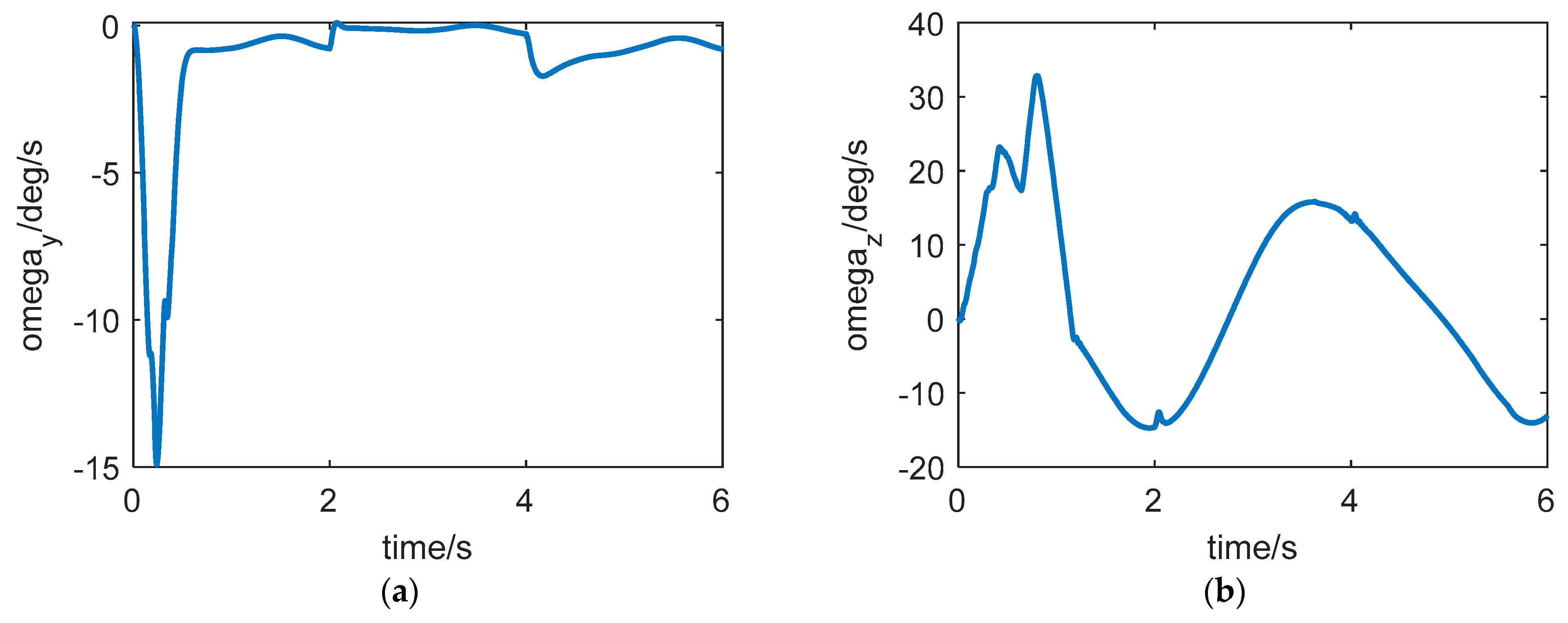
Steady-state responses of the attitude angular rate in Scenario 2. (a) Curve of roll rate . (b) Curve of yaw rate .
Figure 13.
Steady-state responses of the attitude angular rate in Scenario 2. (a) Curve of roll rate . (b) Curve of yaw rate .

Figure 14.
Steady-state responses of overload in Scenario 2. (a) Curve of pitch overload . (b) Curve of yaw overload .
Figure 14.
Steady-state responses of overload in Scenario 2. (a) Curve of pitch overload . (b) Curve of yaw overload .

Figure 15.
Control input of the pitch and yaw channels in Scenario 2. (a) Control input of the pitch channel of ADP-LSTM. (b) Control input of the pitch channel of SMC-RNN. (c) Control input of the yaw channel of ADP-LSTM. (d) Control input of the yaw channel of SMC-RNN.
Figure 15.
Control input of the pitch and yaw channels in Scenario 2. (a) Control input of the pitch channel of ADP-LSTM. (b) Control input of the pitch channel of SMC-RNN. (c) Control input of the yaw channel of ADP-LSTM. (d) Control input of the yaw channel of SMC-RNN.

Figure 16.
Output of LSTM neural network in Scenario 2. (a,b): .

Figure 17.
Weight update of LSTM neural network in Scenario 2. (a) . (b) . (c) .

Figure 18.
Curve of the Hamiltonian function in Scenario 2.

Figure 19.
Control input consumption of ADP-LSTM and SMC-RNN in Scenario 2. (a) Tail fin consumption. (b) Direct force consumption.
Figure 19.
Control input consumption of ADP-LSTM and SMC-RNN in Scenario 2. (a) Tail fin consumption. (b) Direct force consumption.


Table 1.
Aircraft parameters.
| 1200 m/s | 500 kg | 0.048 | 1.500 | 12.101 | 0.166 | 0.004 | 0.024 | 0.604 | 1 m |
Disclaimer/Publisher’s Note: The statements, opinions and data contained in all publications are solely those of the individual author(s) and contributor(s) and not of MDPI and/or the editor(s). MDPI and/or the editor(s) disclaim responsibility for any injury to people or property resulting from any ideas, methods, instructions or products referred to in the content. |
© 2024 by the authors. Licensee MDPI, Basel, Switzerland. This article is an open access article distributed under the terms and conditions of the Creative Commons Attribution (CC BY) license (https://creativecommons.org/licenses/by/4.0/).
Share and Cite
MDPI and ACS Style
Yuan, Y.; Zhou, D. Reinforcement Learning for Dual-Control Aircraft Six-Degree-of-Freedom Attitude Control with System Uncertainty. Aerospace 2024, 11, 281. https://doi.org/10.3390/aerospace11040281
AMA Style
Yuan Y, Zhou D. Reinforcement Learning for Dual-Control Aircraft Six-Degree-of-Freedom Attitude Control with System Uncertainty. Aerospace. 2024; 11(4):281. https://doi.org/10.3390/aerospace11040281
Chicago/Turabian StyleYuan, Yuqi, and Di Zhou. 2024. "Reinforcement Learning for Dual-Control Aircraft Six-Degree-of-Freedom Attitude Control with System Uncertainty" Aerospace 11, no. 4: 281. https://doi.org/10.3390/aerospace11040281
Note that from the first issue of 2016, this journal uses article numbers instead of page numbers. See further details here.