Radio Science Experiments during a Cruise Phase to Uranus

Abstract

The exploration of Uranus, a key archetype for ice giant planets and a gateway to understanding distant exoplanets, is acquiring increasing interest in recent years, especially after the Uranus Orbiter and Probe (UOP) mission has been prioritized in the Planetary Science Decadal Survey 2023–2032. This paper presents the results of numerical simulations aimed at providing experimental constraints on the parameterized post-Newtonian (PPN) parameter $\gamma$, a measure of space–time curvature in general relativity (GR), during the cruise phase of a spacecraft travelling to Uranus. Leveraging advanced radio tracking systems akin to those aboard the JUICE and BepiColombo missions, we explore the potential of solar conjunction experiments (SCEs) to refine current measurements of $\gamma$ by exploiting the spacecraft’s long journey in the outer Solar System. We discuss the anticipated enhancements over previous estimates, underscoring the prospect of detecting violations of GR. Our simulations predict that by using an advanced radio tracking system, it is possible to obtain an improvement in the estimation of $\gamma$ up to more than an order of magnitude with respect to the latest measurement performed by the Cassini–Huygens mission in 2002, contingent on the calibration capabilities against solar plasma noise. The results reveal that a number of SCEs during the mission can substantially strengthen the validation of GR. In tandem with fundamental physics tests, the use of radio links during SCEs presents a valuable opportunity to dissect the solar corona’s plasma dynamics, contributing to solar physics and space weather forecasting. This paper also enumerates methodologies to analyze electron density, localize plasma features, and deduce solar wind velocity, enriching the scientific yield of the experiments beyond the primary objective of testing GR during the cruise phase of a mission to Uranus.

1. Introduction

Uranus is becoming an increasingly meaningful target for deep space exploration missions [1,2]. Significant scientific challenges emerge because of the planet’s unique features, such as its unusually large axial tilt (98°), the consequent atmospheric dynamics [3], and the complex magnetic field [4,5]. Furthermore, recent studies suggest that four of its icy moons (Ariel, Umbriel, Titania, and Oberon) represent potential ocean worlds [6]. This interest is timely, as NASA’s Kepler mission has identified that planets similar in size to Solar System ice giants are the most frequently observed exoplanets (http://exoplanetarchive.ipac.caltech.edu/docs/counts_detail.html, accessed on 20 October 2023), positioning Uranus as a vital analogue to these common distant worlds [7]. Yet, Uranus remains largely unexplored, as only the Voyager 2 spacecraft flew by the planet over three decades ago. The 2023–2032 Decadal Survey has recommended the Uranus Orbiter and Probe (UOP) as the top priority Flagship-class mission for the coming decade [8].

While the cruise phase to Uranus presents logistical and engineering challenges, it also offers unique opportunities for scientific inquiry. The potential for significant scientific outcomes during this phase is amplified by the advancements in state-of-the-art radio tracking systems, as exemplified by radio tracking instrumentation currently operational on ESA’s missions JUICE [9] and BepiColombo [10]. In the cruise phase of interplanetary missions, these systems can play a pivotal role in testing general relativistic effects and studying the solar corona during solar conjunctions (a geometrical configuration in which the Sun–Earth–Probe angle tends to zero, as depicted in Figure 1). A solar conjunction experiment (SCE) is a powerful tool for probing general relativity (GR), providing an estimate of the parameterized post-Newtonian (PPN) parameter $\mathit{\gamma }$. The PPN parameters [11] serve as an effective means to test and compare gravitational theories. Among the ten PPN parameters, the Eddington parameter $\gamma$ (whose value is one in GR) describes the space–time curvature produced by any mass distribution. The tightest experimental constraint on $\gamma$ so far was provided by NASA’s Cassini–Huygens mission in 2002 by analyzing plasma-free Doppler data collected during a solar conjunction [12], indicating that $\left(\gamma -1\right)=\left(2.1\pm 2.3\right)\times {10}^{-5}$, which is thus compatible with general relativity. The Mercury Orbiter Radio science Experiment (MORE) on the ESA/JAXA BepiColombo mission uses an advanced radio tracking system for plasma-free Doppler and range measurements [10]. Currently, it has conducted six SCEs to improve the Cassini result, but its journey in the innermost regions of the Solar System has led the experiments to face limitations caused by the unpredictable fluctuations of solar radiation and wind pressure accelerations [13], which are too small to be calibrated by the onboard accelerometer [14,15]. Consequently, the attainable improvement over Cassini’s result is expected to be limited by a factor of 3–4 depending on the solar activity [16]. In contrast, the 3GM experiment on ESA’s JUICE mission, using similar radio tracking instrumentation onboard the spacecraft, will operate in the calmer outer Solar System [9,17,18,19]. If SCEs are performed during its journey, this could lead to a 14-times more precise measurement than Cassini [20]. The long journey travelled by a spacecraft heading toward Uranus, venturing farther from the Sun compared to these missions, would provide an exquisite opportunity to refine and improve the determination of $\gamma$ upon previous estimates, thereby increasing the possibilities to find a violation of GR, which would be a result of outstanding importance. Furthermore, a violation of GR found by more than one mission would greatly increase the confidence in the result. In addition to this fundamental physics test, radiometric data collected during solar conjunctions can also be exploited to study the solar corona. In [21], the Doppler data collected during the Cassini SCEs have been used to provide the space–time localization of plasma features. In [22], the authors provided measurement of the electron density in the solar corona thanks to VLBI data. This opportunity can provide invaluable insights into solar physics, complementing the SCEs and other scientific objectives of the mission.

A radio science package will likely be hosted onboard the UOP mission to study the gravity field and to investigate the interior structure of Uranus. In this work, we point out some opportunity experiments that can be performed by leveraging on the onboard radio science capabilities while in cruise to Uranus. We describe a numerical simulation carried out to predict the experimental constraint that can be set on $\gamma$ when conducting SCEs during the cruise phase. We also provide a description of the potential scientific return of studying the solar corona with radiometric data collected during the SCEs. The structure of this paper is outlined as follows: Section 2 presents the specifications of the radio tracking apparatus essential for executing these experiments; Section 3 details the methodology employed in this study; Section 4 delineates the properties of the interplanetary trajectory segment analyzed; Section 5 reports a description of the assumptions made for the numerical simulations; Section 6 discusses the findings of this research; in Section 7 we propose a series of potential experiments to investigate the solar corona using conjunction data. Finally, Section 8 draws the conclusions of the work.

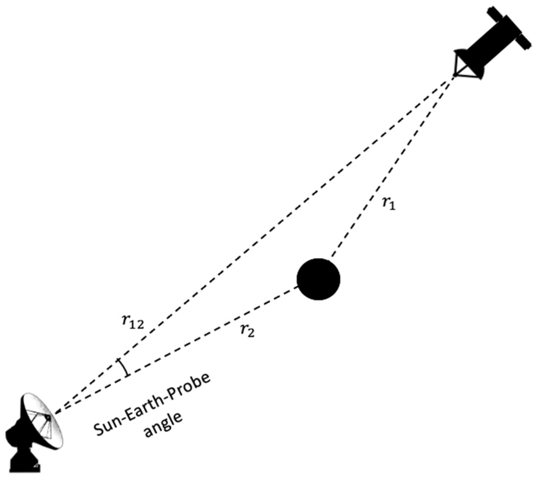
2. Advanced Radio Tracking System for Interplanetary Missions

In this work, we assume that the spacecraft travelling to Uranus hosts radio tracking instrumentation with performance comparable to the one hosted onboard of JUICE or BepiColombo (a necessary requirement to perform SCEs). The system architecture is an evolution of the one used for the radio science experiment of Cassini. The main addition is the inclusion of a pseudo-noise wide band ranging system at 24 Mcps (Mega chips per second), which provides accurate range data [23]. In this work, we conservatively assumed a ranging system at a standard chip rate of 3 Mcps to determine the predicted ranging performance (see Section 5.2). Both range and Doppler observables are available during radio tracking passes, and both are calibrated for the noise due to the solar plasma at almost all solar elongation angles, thanks to a multi-frequency radio link [24]. In addition to the relativistic frequency shift measured by Cassini, the plasma-free range observables allow for a measurement of the relativistic time delay, and this is the key factor that allows for aiming at an improved estimate of $\gamma$ with respect to Cassini, since the Doppler data quality is expected to be comparable. The multi-frequency radio link is enabled by two key elements: the Ka-band transponder, which establishes a coherent two-way Ka/Ka link (≈34 GHz uplink–≈32 GHz downlink), and a deep space transponder (DST), which enables two downlinks at X- and Ka-band (≈8.4 and ≈32 GHz, respectively) coherent with an X-band uplink (≈7.2 GHz). The Integrated Deep Space Transponder (IDST) mounted onboard the VERITAS mission can establish any dual-link combination in X- and Ka-band, providing partial plasma noise calibration [25]. Note that to carry out an SCE, a minimum of three links are required to obtain complete compensation of plasma noise (see Section 3.1). The Ka/Ka link provides the primary measurements for the radio science experiment, while the TT&C (Telemetry, Tracking and Command) X/X and X/Ka links serve for plasma calibrations. All measurements shall be carried out in a coherent two-way mode, in which the frequency reference is generated at the ground station and all onboard transponders are commanded in a coherent mode. At the present day, only two ground stations have full uplink/downlink Ka-band capabilities, allowing for the multi-frequency link: ESA’s DSA-3 antenna at Malargüe, Argentina, and NASA’s DSS 25 located in Goldstone, California. Both are endowed with a water vapor radiometer able to correct for noise introduced by Earth’s troposphere, which is necessary to obtain accurate radiometric data [26,27,28].

3. Method

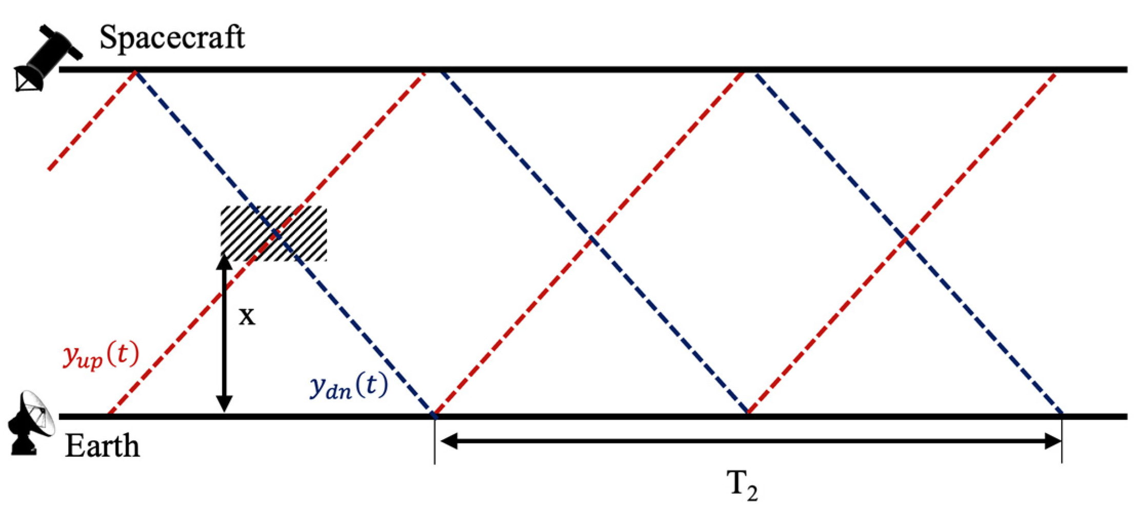
3.1. Calibration of Solar Plasma Dispersive Effects

The multi-frequency link enabled by this tracking system architecture produces six measurable quantities, three range and three Doppler observables, at the $\mathrm{X}/\mathrm{X}\left({\mathrm{z}}_{\mathrm{X}\mathrm{X}}\right), \mathrm{X}/\mathrm{K}\mathrm{a}\left({\mathrm{z}}_{\mathrm{X}\mathrm{K}}\right), \mathrm{a}\mathrm{n}\mathrm{d} \mathrm{K}\mathrm{a}/\mathrm{K}\mathrm{a}\left({\mathrm{z}}_{\mathrm{K}\mathrm{K}}\right)$ frequencies. Note that z can either be interpreted as the range or Doppler observable. The non-dispersive (plasma-calibrated) observable $z_{nd}$, as well as the plasma effect on the uplink (${\mathrm{z}}_{\uparrow })$ and downlink (${\mathrm{z}}_{\downarrow }$) at a baseline frequency, are the unknowns. Neglecting incoherent noise (such as thermal noise of the receiver), the generic radio observable z is the sum of the non-dispersive contribution ${\mathrm{z}}_{\mathrm{n}\mathrm{d}}$, and contributors coming from the path delay in the uplink and downlink (${\mathrm{z}}_{\uparrow }$ and ${\mathrm{z}}_{\downarrow }$). Within the realm of geometric optics, these three indeterminate values can be computed in the linear system as follows:

$$\begin{gathered} {\mathrm{z}}_{\mathrm{X}\mathrm{X}}={\mathrm{z}}_{\mathrm{n}\mathrm{d}}+{\mathrm{z}}_{\uparrow }+\frac{1}{{\mathsf{\alpha }}_{\mathrm{X}\mathrm{X}}^2}{\mathrm{z}}_{\downarrow } \\ {\mathrm{z}}_{\mathrm{X}\mathrm{K}}={\mathrm{z}}_{\mathrm{n}\mathrm{d}}+{\mathrm{z}}_{\uparrow }+\frac{1}{{\mathsf{\alpha }}_{\mathrm{X}\mathrm{K}}^2}{\mathrm{z}}_{\downarrow } \\ {\mathrm{z}}_{\mathrm{K}\mathrm{K}}={\mathrm{z}}_{\mathrm{n}\mathrm{d}}+\frac{1}{{\mathsf{\beta }}^2}{\mathrm{z}}_{\uparrow }+\frac{1}{{\mathsf{\beta }}^2{\mathsf{\alpha }}_{\mathrm{K}\mathrm{K}}^2}{\mathrm{z}}_{\downarrow } \end{gathered}$$

(1)

Here, ${\mathrm{z}}_{\uparrow }$ and ${\mathrm{z}}_{\downarrow }$ are in reference to an X-band uplink carrier, $\beta$ symbolizes the ratio of the uplink frequency in Ka- and X-band, and ${\mathsf{\alpha }}_{\mathrm{K}\mathrm{K}}, {\mathsf{\alpha }}_{\mathrm{X}\mathrm{K}}, \mathrm{a}\mathrm{n}\mathrm{d} {\mathsf{\alpha }}_{\mathrm{X}\mathrm{X}}$ represent the transponder ratios for the Ka/Ka, X/Ka, and X/X links, in that order. Data integrity progressively weakens when the signal path starts travelling deeply into the solar corona, especially at X/X. The operational threshold for the technique compensating for plasma interference cannot be predicted with precision, as it is contingent on the solar activity at the experiment’s time. For the Cassini SCE, conducted near a period of solar peak, the plasma-calibrated Doppler exhibited an Allan deviation of ${10}^{-14}$ at 1000 s of integration time when the impact parameter b (the minimum distance between the light path and the Sun’s center of mass) was beneath 7 solar radii [29]. The cancellation process encountered failure only once during a tracking pass executed when b was under 5 solar radii, due to the X-band link experiencing frequent signal losses. Conversely, during the inaugural SCE of BepiColombo (March 2021, which took place in an ascending phase of the solar cycle, thus close to minimum), plasma cancellation proved highly effective, even when the impact parameter reached its minimum value of about 4 solar radii. The ${\mathrm{z}}_{\mathrm{n}\mathrm{d}}$ is the quantity of interest for the GR tests, containing the information on the Earth–spacecraft motion and the relativistic deflection. The quantities ${\mathrm{z}}_{\uparrow }$ and ${\mathrm{z}}_{\downarrow }$ provide information on the solar plasma and can be used to study properties of the solar corona (details are reported in Section 7).

3.2. Orbit Determination Process

Precise orbit determination (POD) leverages on range and Doppler data collected at a ground station to estimate model parameters. These measurements are processed through sophisticated POD codes. The process involves iterative refinement, comparing the data collected from ground antennas (observed observables) with the predicted value of the observables based on a priori dynamical and observation models (computed observables). To simulate a POD process, synthetic observed observables are generated based on these models (i.e., a “real world” scenario), while the computed observables are produced accounting for possible errors in the model parameters. If both the dynamical and observation models were perfect, the difference between observed and computed observables (residuals, $\mathit{\delta }\mathit{z}$) would contain only measurement noise. On the contrary, signatures in the residuals indicate the need for model adjustments. We adopt a minimum variance least square filter with a priori information to adjust the model parameters and minimize the residuals. The explicit expression of the best estimate of the solve-for parameters is given by [30] the following:

$$\mathit{\delta }\widehat{\mathit{x}}={\left({\mathit{H}}^{\mathit{T}}\mathit{W}\mathit{H}+{\mathit{P}}_{\mathit{A}\mathit{P}}^{-\mathbf{1}}\right)}^{-\mathbf{1}}\left({\mathit{H}}^{\mathit{T}}\mathit{W}\mathit{\delta }\mathit{z}+{\mathit{P}}_{\mathit{A}\mathit{P}}^{-\mathbf{1}}\mathit{\delta }{\mathit{x}}_{\mathit{A}\mathit{P}}\right)$$

(2)

where $\mathit{\delta }\widehat{\mathit{x}}$ is the n-dimensional vector of the correction on the solve-for model parameters, H is the design matrix (containing the partial derivatives of the observables z with respect to $\widehat{\mathit{x}}$), W is the weight matrix, and $\mathit{\delta }{\mathit{x}}_{\mathit{A}\mathit{P}}$ and ${\mathit{P}}_{\mathit{A}\mathit{P}}$ are, respectively, the a priori estimate of $\widehat{\mathit{x}}$ with respect to the reference trajectory and its covariance matrix.

In an SCE, the PPN parameter $\gamma$ is included in the list of estimated model parameters. Indeed, the curvature of space–time near massive bodies like the Sun causes a deflection of the path of the radio signal exchanged between the Earth station and the spacecraft, as predicted by GR. While the spacecraft approaches a solar conjunction, this effect magnifies, providing an opportunity for easier detection of it. In a PPN formalism, the associated time delay and frequency shift can be expressed as functions of $\gamma$. During a solar conjunction, it is possible to approximate the expression of these quantities as the following [31]:

$$\mathsf{\Delta }T=\frac{\left(1+\gamma \right)G{M}_{\odot }}{c^3}ln \left(\frac{r_1{r}_2}{b^2} \right)$$

(3)

$$\frac{\mathsf{\Delta }\nu }{\nu }=\frac{d\Delta T}{dt}=-2\frac{\left(1+\gamma \right)G{M}_{\odot }}{c^{3}b}\frac{db}{dt}$$

(4)

where $M_{\odot }$ is the mass of the Sun, G is the Newtonian gravitational constant, and c is the speed of light in vacuum (refer to Figure 1 for the definition of $r_1$ and $r_2$). Notice that the time delay increases with small impact parameter of the signal while the frequency shift is proportional to its temporal rate of change, which depends on the observation geometry. Both these effects must be considered for an observation model aimed at reproducing the expected value of range and Doppler observables.

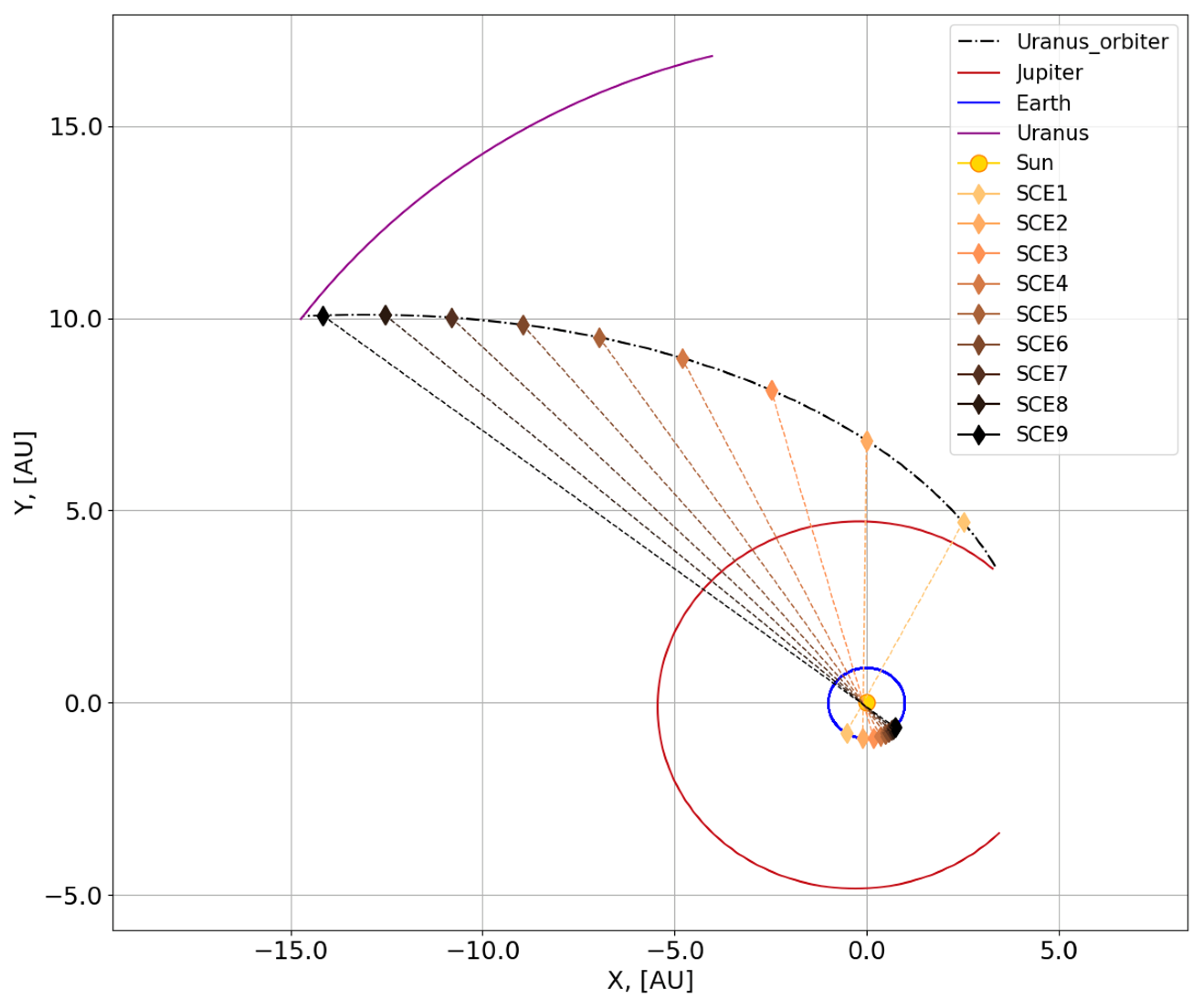
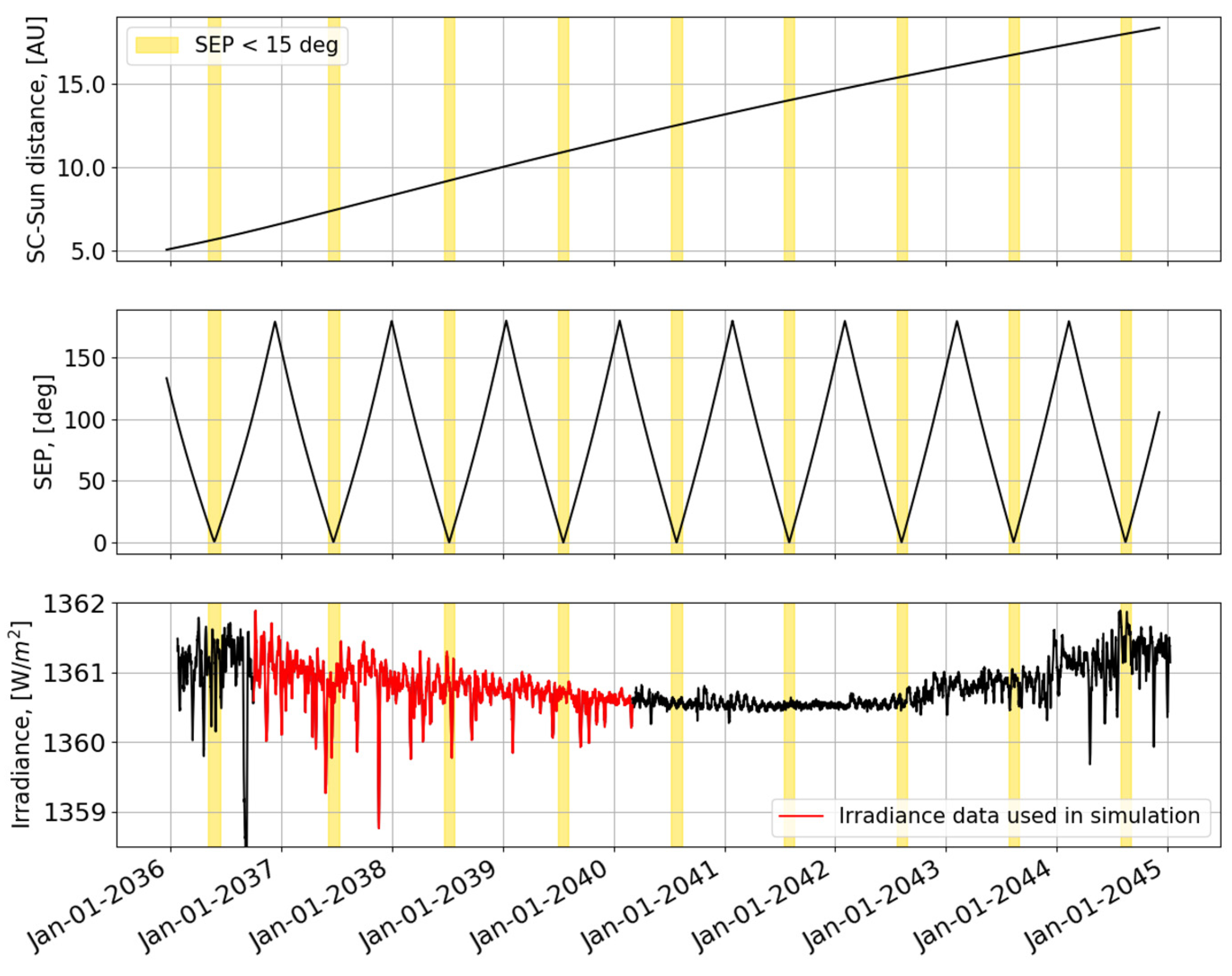
4. Interplanetary Trajectory

To test GR, the spacecraft must serve as a stable platform to minimize unmodeled dynamic perturbations [32]. In this study, we consider a spacecraft’s trajectory en route to Uranus post-Jupiter flyby (Figure 2). We chose this 9-year trajectory segment (2035–2044) to identify conjunctions far enough from the Sun to significantly reduce Sun-induced disturbances, even during solar maximum. Note that an accurate trajectory to Uranus is not required at this stage. Over the 9-year journey to Uranus, the Sun–Earth–Probe angle will annually approach zero (Figure 3, center panel), with an equal number of solar oppositions occurring. As Section 3.2 discusses, relativistic signals more strongly influence Doppler data during rapid conjunctions, while range data’s contribution is heightened with smaller minimum impact parameters. The use of both data types ensures optimal performance. The conjunctions reported in Figure 2 are characterized by a minimum impact parameter < 4 solar radii, while its maximum rate of change is always >3 solar radii per day (as a comparison, for BepiColombo SCEs the minimum b was about 4 solar radii in June 2023 with a maximum rate of change equal to 3.9 solar radii per day). All solar conjunctions occur beyond 5 Astronomical Unit (AU) from the Sun, and starting from the fourth one, each subsequent experiment takes place over 10 AU away (Figure 3, top panel). Scheduled between 2036 and 2045, the first and last two experiments coincide with a solar maximum (≈2036–2037, ≈2043–2044), while five occur during a solar minimum (≈2038–2042), considering the 11-year solar cycle (Figure 3, bottom panel). These five conjunctions provide prime conditions for testing GR: reduced random accelerations due to the spacecraft’s distance from the Sun ensure more stable dynamics; a dimmer solar activity means less perturbation in the plasma environment near the solar corona, facilitating high-quality plasma calibrations to smaller impact parameters. This setting is optimal for collecting range data when relativistic effects peak, allowing for a refined estimate of $\gamma$.

5. Numerical Simulations

In Section 5.1 and Section 5.2, we describe the dynamical and observation model used to generate synthetic observed observables. In Section 5.3, we show the perturbed models used to simulate computed observables, reflecting possible errors in model parameters. The numerical simulations presented in this work have been carried out with the orbit determination software MONTE v149 (mission analysis operations and navigation toolkit environment), developed by NASA JPL [33].

5.1. Dynamical Model

To generate the reference trajectory, we considered that the spacecraft is travelling from Jupiter to Uranus under the effect of the gravity of the Sun, the planets, and all the major bodies of the Solar System, represented in a relativistic PPN framework. We used the JPL’s de440 ephemerides to account for the dynamics of all the Solar System bodies [34].

The effect of the anisotropic thermal emission of the spacecraft, mainly due to the onboard radioisotope thermoelectric generators (RTGs), has been included in the model. The corresponding acceleration vector can be expressed as follows:

$${\mathbf{a}}_{\mathbf{R}\mathbf{T}\mathbf{G}}={\mathit{A}}_{\mathit{R}\mathit{T}\mathit{G}}{e}^{-\frac{t-t_0}{\tau }}$$

(5)

where $\tau$ is the exponential time constant ($\tau =2.734\times {10}^9 \mathrm{s}$, the half-life of plutonium 238). At this stage, there is no detailed information about the UOP RTGs, so we assumed the estimates provided by the navigation of the Cassini spacecraft [12]: ${\mathit{A}}_{\mathit{R}\mathit{T}\mathit{G}}$ is a constant vector with components equal to $3\times {10}^{-9} \mathrm{m}/{\mathrm{s}}^2$along the spacecraft–Earth direction, $1\times {10}^{-10} \mathrm{m}/{\mathrm{s}}^2$ orthogonal to the orbital plane, and $4\times {10}^{-10} \mathrm{m}/{\mathrm{s}}^2$ in the orbital plane, orthogonal to the spacecraft–Earth direction [10]. Indeed, the actual values will be different, depending on the location and orientation (thus, on the acceleration asymmetry) of the RTGs onboard the spacecraft, but will likely have comparable order of magnitude; for example, in the case of New Horizon, the acceleration due to the RTG in the spacecraft–Earth direction for the period between February 2008 and May 2013 has been estimated at the level of $\approx 1\times {10}^{-9} \mathrm{m}/{\mathrm{s}}^2$ [35].

We simulated the solar radiation pressure acting on the spacecraft, which can be expressed as the following [36]:

$${\mathbf{a}}_{\mathbf{S}\mathbf{R}\mathbf{P},\mathbf{k}}=-\frac{{\mathsf{\varphi }}_{1\mathrm{A}\mathrm{U}}\left(t\right)}{\mathrm{c}}{\frac{{\mathrm{A}}_{\mathrm{k}}{(\widehat{\mathbf{n}}}_{\mathbf{k}}\cdot \widehat{\mathbf{s}})}{{\mathrm{m}}_{\mathrm{s}\mathrm{c}}}\left(\frac{{\mathrm{R}}_{\mathrm{E}\mathrm{S}}}{{\mathrm{D}}_{\mathrm{s}}\left(\mathrm{t}\right)}\right)}^2\left[\left(1-{\mathrm{c}}_{\mathrm{s},\mathrm{k}}\right)\widehat{\mathbf{s}}+2\left({\mathrm{c}}_{\mathrm{s},\mathrm{k}}\left(\widehat{\mathbf{s}}·{\widehat{\mathbf{n}}}_{\mathit{k}}\right)+\frac{{\mathrm{c}}_{\mathrm{d},\mathrm{k}}}{3}\right){\widehat{\mathbf{n}}}_{\mathit{k}}\right]$$

(6)

where $\widehat{\mathbf{s}}$ and ${\widehat{\mathbf{n}}}_{\mathit{k}}$ are, respectively, the direction pointing from the spacecraft toward the Sun and the normal direction to the exposed surfaces, ${\mathrm{m}}_{\mathrm{s}\mathrm{c}}$ is the mass of the spacecraft, ${\mathrm{A}}_{\mathrm{k}}$ is the area of the considered spacecraft plate element, $c_{s,k}$ and $c_{d,k}$ are the specular and diffuse reflectivity coefficients of the surfaces, ${\mathrm{D}}_{\mathrm{s}}\left(\mathrm{t}\right)$ is the spacecraft–Sun distance, ${\mathrm{R}}_{\mathrm{E}\mathrm{S}}$ corresponds to 1 AU, and ${\mathsf{\varphi }}_{1\mathrm{A}\mathrm{U}}\left(t\right)$ is the solar irradiance at 1 AU from the Sun. The overall SRP acceleration acting on the spacecraft is then obtained considering all the surface elements. Following the indications reported in [37], we assumed a cylindrical spacecraft with a height of 7.1 m and a diameter of 1.8 m, endowed with a 3.1 m high gain antenna (the total area of the spacecraft bus exposed to the Sun is about $20 {\mathrm{m}}^2$); the mass of the spacecraft decreases linearly from a launch mass of 7235 kg (considering launch in 2031) to a mass at the time of the Uranus orbit insertion of 4919 kg. We assumed typical values for the spacecraft surfaces’ thermo-optical coefficients: for the spacecraft bus, we considered $c_{s,BUS}=0.032$ and $c_{d, BUS}=0.105$ while for the high gain antenna we fixed $c_{s,HGA}=0.072$ and $c_{d,HGA}=0.528$. The total solar irradiance (TSI) ${\varphi }_{1AU}\left(t\right)$ presents random temporal variations (up to 0.1% of the central value in a few days) due to the presence of sunspots and bright faculae over the Sun’s surface [38]. During the first SCE, the SRP is ${\approx 5\times 10}^{-10} \mathrm{m}/{\mathrm{s}}^2$, while the acceleration due to irradiance variations is at the level of a few parts in ${10}^{-13} \mathrm{m}/{\mathrm{s}}^2$. To model this effect, we used the 6-hour irradiance measurements [39] of the space-based radiometer TIM [40].

The dynamical pressure induced by the solar wind produces an acceleration at a similar level (${10}^{-14}–{10}^{-13} \mathrm{m}/{\mathrm{s}}^2$, depending on the solar activity); during particular events, like coronal mass ejections impacting the spacecraft’s surfaces, this effect could reach peaks up to the level of $\approx 10^{-11}\mathrm{m}/{\mathrm{s}}^2$. The corresponding acceleration is modeled as follows [41]:

$${\mathit{a}}_{\mathit{s}\mathit{w},\mathit{k}}=\frac{1}{2}\rho C_D\frac{A_k}{m_{sc}}{V}^2 \widehat{\mathit{V}}$$

(7)

where $\rho =m_{p}n$ with $m_p$being the proton mass and $n$ being the density of the charged particles (particles/$\mathrm{c}{\mathrm{m}}^3$), V is the relative velocity between the solar wind and the spacecraft element k, and $C_D$is the drag coefficient (we assumed $C_D=1$ to account for full absorption). To represent this effect, we used 1-hour data of the average velocity V and the proton density n from NASA/GSFC’s OMNI dataset through OMNIWeb [42].

Due to the stochastic nature of the solar activity, we repeated the simulation using 100 different realizations of solar irradiance and solar wind accelerations, generating a set of 100 reference trajectories. To consider a worst-case scenario, these SRP and solar wind models are produced with data from the period 2003–2007, close to a solar maximum (see, for example, the red TSI data in Figure 3, bottom panel). For each of these trajectories, we simulated the corresponding set of range and Doppler observables.

5.2. Generation of Synthetic Observed Observables

Following the indications reported in [37], we simulated radiometric data collected from the Deep Space Network’s (DSN) 34 m beam waveguide antenna DSS 25. The maximum elevation from DSS 25 ranges between 60 and 80 deg for the nine experiments. We considered an elevation mask of 10 degrees to discard low-elevation data, which are most affected by Earth’s troposphere. We generated synthetic Doppler data every 60 s and range data every 2 s, with an accuracy of $12 \mathsf{\mu }\mathrm{m}/\mathrm{s}$ (in terms of range rate) and $40 \mathrm{c}\mathrm{m},$ respectively. The accuracy on range measurements was computed based on a link budget accounting for the in-flight performance of the BepiColombo radio tracking system [43] but conservatively assuming a chip rate of 3 Mcps. The relativistic time-delay and frequency shift were modeled according to the formulation reported in [44]. We assumed that each SCE lasts 12 days, a period in which any wheel-off-loading maneuver shall be avoided. The assumption of a good reconstruction of the attitude of each spacecraft element is fundamental for a precise GR test. An accuracy of about 0.1° in the reconstruction of the spacecraft orientation, attainable with modern attitude control systems, would be sufficient for the purposes of the SCE [45]. As mentioned in Section 3.2, when the impact parameter of the signal is too close to the solar corona, the plasma noise cancellation scheme could fail. There is no clear indication to predict when this may happen, but with strong solar activity one may expect that the scintillation regime emerges at larger impact parameter with respect to a case of faint solar activity. In Section 6, we report the result of the simulation for a baseline value of the impact parameter threshold of 4 solar radii; then, to account for different scenarios, we repeated simulations with several assumptions on the impact parameter threshold ranging from 7 to 4 solar radii.

5.3. Simulation of the Orbit Determination Process

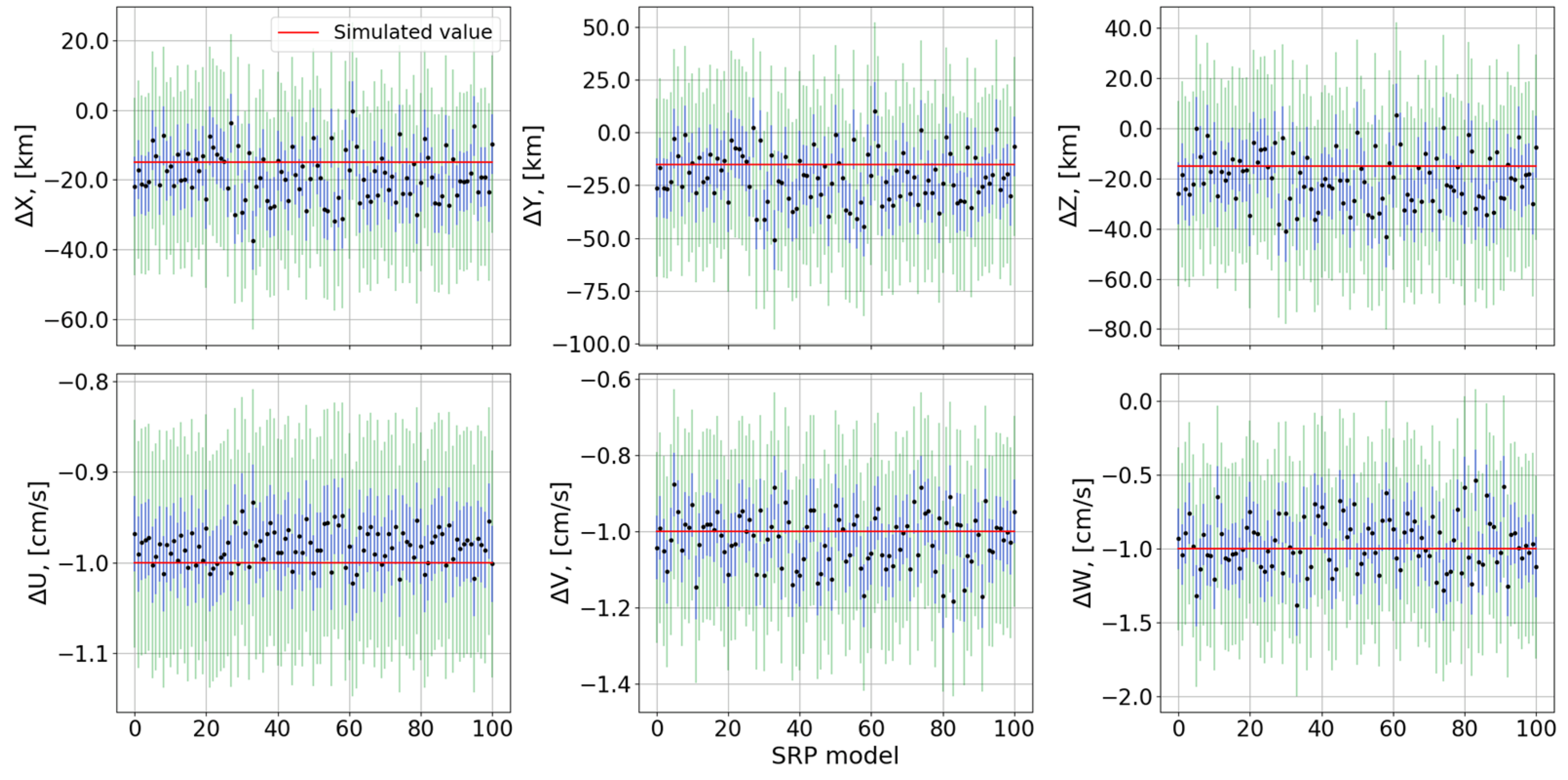
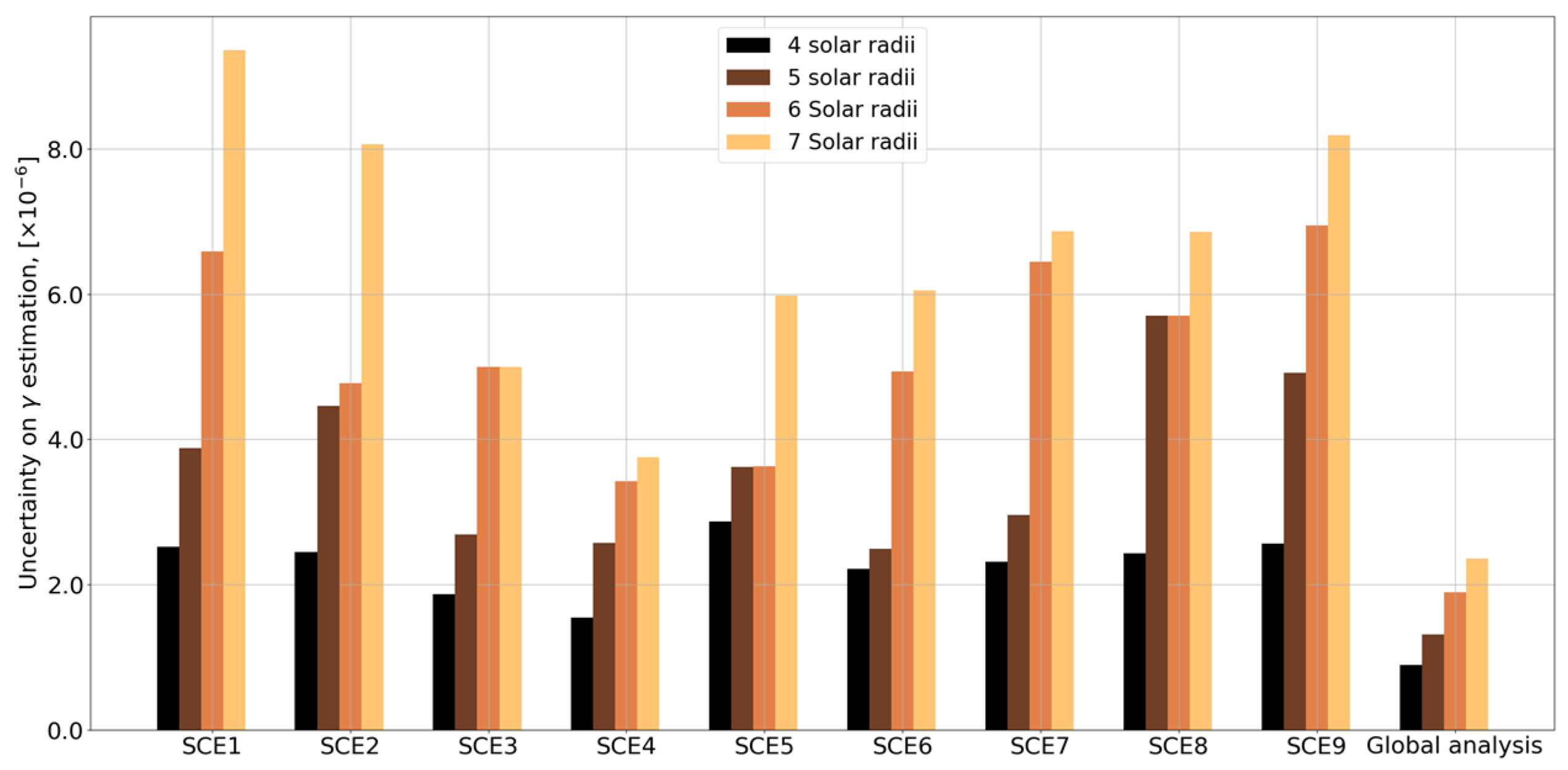
The synthetic data were used in a standard orbit determination process, as outlined in Section 3.2. The spacecraft’s state vector carries an assumed error of 15 km in position and 1 cm/s in velocity. To account for unknown solar activity, the TSI was set constant, and the solar wind effect was not included in the model. The model deliberately excludes the acceleration induced by the RTG, simulating a situation where its precise value is not well known. The spacecraft bus’s absorptivity is assumed to have a $\approx$7% deviation from the nominal value. Moreover, a systematic range bias of 60 cm was incorporated.

To rectify errors in these model parameters, corrections were made for the spacecraft state vector at the beginning of the observation arc, the spacecraft bus’s absorptivity, RTG acceleration components, a range bias, and the PPN parameter $\gamma$, which is the focus of the experiment. Ground station coordinates were also estimated to account for the related uncertainties in the final covariance solution. The orbit determination procedure was repeated using synthetic observables derived from 100 solar-induced dynamic perturbation models for each experiment. This was to examine if, despite model inaccuracies and unmodeled TSI variations, an unbiased estimate of $\gamma$ could be achieved. Data considered in this analysis were plasma-calibrated up to 4 solar radii.

Table 1. Nominal value, a priori uncertainties, and mismodeling on the estimated parameters.

Parameter	Nominal Value	A Priori Uncertainty	Perturbation
[x, y, z]	From reference trajectory	100 km	15 km
[u, v, w]	From reference trajectory	1 m/s	1 cm/s
Absorptivity	0.86	0.06	−0.06
Range bias	0 cm	100 km	60 cm
${\mathbf{a}}_{\mathbf{R}\mathbf{T}\mathbf{G}}$	$\left[3, 0.1, 0.4\right]\times 10^{-9} \mathrm{m}/{\mathrm{s}}^2$	$10^{-6} \mathrm{m}/{\mathrm{s}}^2$	$-\left[3, 0.1, 0.4\right]\times 10^{-9} \mathrm{m}/{\mathrm{s}}^2$
$\gamma$	1	$10^{-4}$	0
DSS 25 offset [x, y, z]	[0, 0, 0] m	10 cm	[0, 0, 0] m

summarizes the nominal values and the mismodeling on the solve-for model parameters considered to simulate the orbit determination process.

6. Results

The orbit determination filter was able to provide a good fit of the residuals for all nine experiments, despite the introduced mismodeling. Consistently across 100 simulations, an unbiased estimation of $\gamma$ was attainable, with formal uncertainties detailed in

Table 2. Predicted estimation accuracy on $\gamma$ obtained in each solar conjunction for the case of plasma calibrations available up to 4 solar radii.

SCE	${\mathit{\sigma }}_{\mathit{\gamma }}\cdot {10}^{-6}$
1	2.5
2	$2.4$
3	$1.9$
4	$1.5$
5	$2.9$
6	$2.2$
7	$2.3$
8	$2.4$
9	$2.6$
Global analysis	0.71

for each SCE. The most precise constraint on $\gamma$ emerged from SCE #4, achieving an accuracy of $1.5\times {10}^{-6},$ and similar results are obtained by other conjunctions. Figure 4 displays the estimated corrections on the spacecraft state vector components in the Earth Mean Equator at J2000 reference frame during experiment #3 (as an example) with the corresponding formal uncertainties. Repeating these nine SCEs throughout the cruise would corroborate the result, imposing a robust check on GR. Alternatively, combining data from all nine experiments could tighten the constraint on $\gamma$ further, estimating it with a formal uncertainty of $7.1\times {10}^{-7}.$ This analysis, even when applied across 100 varied SRP models, confirmed the unbiased nature of the estimation of $\gamma$.

We also repeated both these simulations in case the solar conditions are more turbulent, impairing the effectiveness of plasma calibrations to higher impact parameters. The corresponding uncertainties in the estimation of $\gamma$ are reported in Figure 5, considering a threshold value of the impact parameter ${\mathrm{b}}_{\mathrm{M}\mathrm{I}\mathrm{N}}$ varying from 7 solar radii (the limit value in the case of Cassini) to 4 solar radii (the minimum value sampled in BepiColombo SCE). Even in the worst case (${\mathrm{b}}_{\mathrm{M}\mathrm{I}\mathrm{N}}=7$ solar radii), the best attainable estimation accuracy on $\gamma$ given by a single SCE is obtained in the last experiment, equal to $3.7\times {10}^{-6}$. Combining data from the nine conjunctions would improve this result by about a factor of two. An experiment providing a similar constraint on the value of $\gamma$ would mark a significant step forward in the experimental verification of general relativity. Existing scalar–tensor theories of gravity predict deviations of the post-Newtonian effects for $\gamma$ at the level of $\left[{10}^{-5};5\times {10}^{-8}\right]$ [46,47], providing a strong motivation to conduct these experiments.

7. Study of the Solar Corona

Spacecraft-based radio signal analysis has been instrumental in probing the heliosphere’s plasma dynamics both within and beyond the ecliptic plane, enabling the examination of regions and scales unattainable by other methods. The urgency to unravel and forecast space weather patterns—known to disrupt satellite operations and impede human activities in space at 1 AU—has heightened the relevance of such studies. Here, we outline a series of potential analyses achievable through the examination of radiometric data, which will be gathered during the solar conjunctions as a spacecraft makes its way toward Uranus. Note that these experiments do not need any additional operation on the spacecraft and ground segment with respect to the relativity test.

7.1. Analysis of Electron Density

Analyzing the plasma content extracted from range measurements, it is possible to obtain information about the electron density in the solar corona. The delay due to the solar plasma affecting range data can be written as a function of the electron density by integrating along the ray path S [48]:

$$d_p={\int }_S^{ }\left(n-1\right)ds=\frac{e^2}{2{ϵ}_0{m}_e{\omega }^2}{\int }_S^{ }{N}_e\left(s\right)ds$$

(8)

where $n=1-\frac{N_e{e}^2}{2{ϵ}_0{m}_e{\omega }^2}$ is the refraction index, $e$ is the electron charge, $m_e$is the electron mass, ${ϵ}_0$ is the permittivity of free space, and $\omega =2\pi f$, with f being the carrier’s frequency. A simple electron density model for the Sun assumes it to be radially symmetric and usually follows a power law depending on the distance r (in solar radii) from the heliocenter:

$$N_e\left(r\right)=N_0{r}^{-{\beta }_e}$$

(9)

where $N_0$ is the fictitious electron density, and${\beta }_e$ is the falloff exponent, usually assumed to be equal to two. For heliocentric distances of less than four solar radii, additional terms of higher order are generally adopted [49]. As described in Section 3.1, the linear system shown in Equation (1) provides the uplink and downlink dispersive contribution on radiometric data ${\mathrm{z}}_{\uparrow }+{\mathrm{z}}_{\downarrow }$ (here, z refers to range observables). By applying calibrations of the effect of Earth’s ionosphere coming from GNSS (Global Navigation Satellite System) measurements [50], it is possible to isolate a measure of the delay due to the solar plasma, $d_p$ only. Using a least square method to fit plasma delay data with a suitable electron density model, it is possible to retrieve the parameters of the model (such as $N_0$ and ${\beta }_e$ of Equation (9), if b > 4 solar radii).

7.2. Space–Time Localization of Plasma Features

A notable application of plasma content measurements involves pinpointing plasma structures along the line of sight [21]. This process entails calculating the cross-correlation between the uplink and downlink plasma-induced fluctuations in Doppler data, with peaks in correlation indicating the presence of a large plasma feature somewhere along the path. As depicted in Figure 6, the ground station and spacecraft are engaged in a continuous exchange of microwave signals. A plasma concentration at a specific distance from the Earth station along the line of sight, x, causes phase perturbations on both uplink and downlink signals, resulting in two distinct signatures in the two-way tracking data. These events are temporally separated by a time lag ${\tau }_s=T_2-2x/c$, with $T_2$ representing the round-trip light time. The temporal gap between these plasma-related occurrences in the Doppler time series can be measured through cross-correlation, enabling the determination of the plasma feature’s distance from Earth. With the ground antenna directed at the spacecraft’s precisely known location, this method facilitates the temporal and three-dimensional spatial localization of plasma events. In the simplified scenario where the plasma screen is geometrically thin, the uplink and downlink paths intersect the screen at a single point, resulting in identical phase shifts for both signals. Consequently, the Doppler time series for the uplink and downlink are precisely temporally displaced duplicates of one another, yielding a cross-correlation function value of one at the lag of $T_2-2x/c$. For a plasma screen with some thickness, the traversed segments for uplink and downlink differ. As such, the respective time series no longer mirror each other, diminishing the peak cross-correlation values below one. The deviation of the cross-correlation function from unity serves as a constraint on the thickness of the plasma screen that predominates the observed Doppler scintillation (other noise sources are negligible during solar conjunctions).

7.3. Estimation of Solar Wind Velocity

Radio waves traversing the solar corona are scattered by density fluctuations within the solar wind, resulting in a diffraction pattern observed on Earth as intensity scintillation [51] of the electric field’s signal measured at the receiving station. The scintillation spectrum thus embodies the spatial structure of the coronal plasma and the velocity of the solar wind. Given the sharp increase in plasma density closer to the Sun, the radio wave’s interaction with the medium can be approximated by a thin phase screen at the closest solar approach. Under these conditions, one can adopt the weak scattering assumption. The density spectrum model is chosen to be spherically symmetric, decaying as ${\Phi }_n\propto r^{-{\beta }_d}$ with distance r referring to the point nearest to the Sun. The solar wind is presumed to exhibit mature turbulence, and the expected value of ${\beta }_d$ for a Kolmogorov-like spectrum in the inertial subrange is $2/3.$ Additionally, ${\Phi }_n\left(k\right)$ adheres to a power-law distribution, ${\Phi }_n\propto k^{-{\alpha }^{\prime }},$ with wavevector $k$ and exponent ${\alpha }^{\prime }$, which may change gradually with $k$ [51].

A practical model for the intensity scintillation spectrum is given by the following [51,52]:

$$P\left(f\right)=\frac{2\pi {\left(\lambda r_e\right)}^2}{V}{\int }_{-\infty }^{+\infty }{\Phi }_n\left(k_x=\frac{2\pi }{V}{f}_{FL},k_y\right)F_{diff}\left(k\right)d{k}_y$$

(10)

where V is the solar wind velocity, $f_{FL}$is the frequency of fluctuations, $\lambda$is the radio signal wavelength, $r_e$ is the classical electron radius, $k_x$ is the wavenumber along the radial direction, and $k_y$ is the wavenumber orthogonal to both the radial direction and the microwave signal path. $F_{diff}\left(k\right)$ denotes the Fresnel propagation filter, a high pass filter that blocks wavenumbers beneath $k_F=\pi /{\left(\lambda z\right)}^{\frac{1}{2}}$, expressed as follows:

$$F_{diff}\left(k\right)=4{\sin }^2\left(k^2\frac{\lambda z}{4\pi }\right)$$

(11)

with $k=\sqrt{k_x^2+k_y^2}$ and $z=\frac{L_1{L}_2}{L_1+L_2}$, where $L_1$ is the distance from the spacecraft to the closest approach, and $L_2$ is the distance from the closest approach to the receiver. The spatial spectrum of plasma density, ${\Phi }_n$, is expressed as follows:

$${\Phi }_n\left(k\right)=A{\left(\sqrt{k_x^2+\frac{k_y^2}{A{R}^2}}\right)}^{-{\alpha }^{\prime }}\exp \left(-\frac{k^2}{k_c^2}\right)r^{-4}$$

(12)

Here, A is a scaling constant, AR is the axial ratio indicating the anisotropy of density irregularities, ${\alpha }^{\prime }$ is the power-law exponent of the turbulence spectrum, and $k_c$ is the wavenumber marking the onset of turbulence dissipation, related to the inner scale $S_i$ by $S_i=3/k_c$.

To estimate the solar wind velocity V and other model parameters of interest (A, $AR$, ${\alpha }^{\prime }$, and $k_c$), the model reported in Equation (10) can be fitted to the observed intensity scintillation spectrum, derived from open-loop data.

8. Conclusions

This study presents a comprehensive assessment of the scientific potential of conducting SCEs during the Uranus Orbiter and Probe’s cruise phase toward Uranus. Our numerical simulations demonstrate that utilizing state-of-the-art radiotracking systems can yield unprecedented precision in measuring the PPN parameter $\gamma$, potentially surpassing previous constraints. The unique trajectory of a spacecraft en route to Uranus, and the advantageous area-to-mass ratio, offer a significant advantage point for these measurements, substantially mitigating the influence of solar radiation pressure variations experienced by missions in the inner Solar System. By simulating the effect of irradiance fluctuations and other model parameter errors in the analysis, we verified that an unbiased estimate of $\gamma$ can be obtained with an accuracy at the 1-σ level of $1.5\times {10}^{-6}$ with just 12 days of plasma-free data collected with an impact parameter larger than 4 solar radii. Similar results can be obtained by the other eight experiments. Using a joint dataset including all nine conjunctions occurring during the cruise phase would tighten this constraint by a factor of $\approx$2. We also reported the attainable results with different assumptions about plasma-calibration efficiency, proving that even with unfavorable solar conditions it is possible to estimate $\gamma$ at the level of $1.9\times {10}^{-6}.$ The reported estimation accuracies can be further improved with more optimistic hypothesis, as, for example, a longer observation timespan or less conservative assumptions on the performance of range data. However, this case requires more attention, and in particular a compensation strategy for unknown solar-induced time-variable disturbances would be required.

Moreover, our study highlights the two-fold scientific interest of performing SCEs, not only in testing relativistic gravity with exquisite accuracy but also in contributing valuable data to solar corona research. The radiometric data acquired during these conjunctions, when analyzed meticulously, could enhance our understanding of solar wind dynamics and electron density distribution within the corona. This dual capability reinforces the importance of SCEs as a versatile tool for advancing research both in fundamental physics and solar physics. In light of these findings, we advocate for the inclusion of SCEs in the mission plan for the Uranus Orbiter and Probe with appropriate radio tracking instrumentation. By leveraging the extended cruise phase, the onboard radio science package, and the probe’s favorable positioning, we can significantly refine our comprehension of space–time curvature effects and solar corona phenomena.

References

1. Hueso, R. The Ice Giants Uranus and Neptune: Current Data and Future Exploration. In Planetary Systems Now; World Scientific (Europe): London, UK, 2023; pp. 211–233. [Google Scholar] [CrossRef]
2. Witze, A. Next stop, Uranus? Icy planet tops priority list for next big NASA mission. Nature 2022, 604, 607. [Google Scholar] [CrossRef] [PubMed]
3. Hammel, H.B. The Ice Giant Systems of Uranus and Neptune. In Solar System Update; Springer: Berlin/Heidelberg, Germany, 2006; pp. 251–265. [Google Scholar] [CrossRef]
4. Stanley, S.; Bloxham, J. Convective-region geometry as the cause of Uranus’ and Neptune’s unusual magnetic fields. Nature 2004, 428, 151–153. [Google Scholar] [CrossRef]
5. Stanley, S.; Bloxham, J. Numerical dynamo models of Uranus’ and Neptune’s magnetic fields. Icarus 2006, 184, 556–572. [Google Scholar] [CrossRef]
6. Castillo-Rogez, J.; Weiss, B.; Beddingfield, C.; Biersteker, J.; Cartwright, R.; Goode, A.; Daswani, M.M.; Neveu, M. Compositions and Interior Structures of the Large Moons of Uranus and Implications for Future Spacecraft Observations. J. Geophys. Res. Planets 2023, 128, e2022JE007432. [Google Scholar] [CrossRef] [PubMed]
7. Rogers, L.A. MOST 1.6 Earth-radius planets are not rocky. Astrophys. J. 2015, 801, 41. [Google Scholar] [CrossRef]
8. National Academy of Sciences, Engineering and Medicine. Origins, Worlds, and Life; National Academies Press: Washington, DC, USA, 2023. [Google Scholar] [CrossRef]
9. Cappuccio, P.; Di Benedetto, M.; Cascioli, G.; Iess, L. Analysis of the 3GM gravity experiment of ESA’s JUICE mission. Adv. Astronaut. Sci. 2018, 167, 3551–3561. [Google Scholar]
10. Iess, L.; Asmar, S.W.; Cappuccio, P.; Cascioli, G.; De Marchi, F.; di Stefano, I.; Genova, A.; Ashby, N.; Barriot, J.P.; Bender, P.; et al. Gravity, Geodesy and Fundamental Physics with BepiColombo’s MORE Investigation. Space Sci. Rev. 2021, 217, 21. [Google Scholar] [CrossRef]
11. Will, C.M. Theory and Experiment in Gravitational Physics; Cambridge University Press: Cambridge, UK, 2018. [Google Scholar]
12. Bertotti, B.; Iess, L.; Tortora, P. A test of general relativity using radio links with the Cassini spacecraft. Nature 2003, 425, 374–376. [Google Scholar] [CrossRef] [PubMed]
13. di Stefano, I.; Cappuccio, P.; Iess, L. Analysis on the solar irradiance fluctuations effect on the bepicolombo superior conjunction experiment. In 2019 IEEE International Workshop on Metrology for AeroSpace, MetroAeroSpace 2019-Proceedings; IEEE: Piscataway, NJ, USA, 2019. [Google Scholar] [CrossRef]
14. di Stefano, I.; Cascioli, G.; Iess, L.; Cappuccio, P. Environmental disturbances on missions for precise tests of relativistic gravity and solar system dynamics: The bepicolombo case. In International Astronautical Congress, IAC; International Astronautical Federation: Paris, France, 2019. [Google Scholar]
15. Santoli, F.; Fiorenza, E.; Lefevre, C.; Lucchesi, D.M.; Lucente, M.; Magnafico, C.; Morbidini, A.; Peron, R.; Iafolla, V. ISA, a High Sensitivity Accelerometer in the Interplanetary Space. Space Sci. Rev. 2020, 216, 145. [Google Scholar] [CrossRef]
16. di Stefano, I.; Cappuccio, P.; Iess, L. The BepiColombo solar conjunction experiments revisited. Class. Quantum Gravity 2021, 38, 055002. [Google Scholar] [CrossRef]
17. Cappuccio, P.; Hickey, A.; Durante, D.; Di Benedetto, M.; Iess, L.; De Marchi, F.; Plainaki, C.; Milillo, A.; Mura, A. Ganymede’s gravity, tides and rotational state from JUICE’s 3GM experiment simulation. Planet Space Sci. 2020, 187, 104902. [Google Scholar] [CrossRef]
18. Shapira, A.; Stern, A.; Prazot, S.; Mann, R.; Barash, Y.; Detoma, E.; Levy, B. An Ultra Stable Oscillator for the 3GM experiment of the JUICE mission. In 2016 European Frequency and Time Forum (EFTF); IEEE: Piscataway, NJ, USA, 2016. [Google Scholar] [CrossRef]
19. Fabrizio, D.M.; Gaetano, D.A.; Giuseppe, M.; Paolo, C.; Ivan, D.S.; Mauro, D.B.; Luciano, I. Observability of Ganymede’s gravity anomalies related to surface features by the 3GM experiment onboard ESA’s JUpiter ICy moons Explorer (JUICE) mission. Icarus 2021, 354, 114003. [Google Scholar] [CrossRef]
20. di Stefano, I.; Cappuccio, P.; Di Benedetto, M.; Iess, L. A test of general relativity with ESA’s JUICE mission. Adv. Space Res. 2022, 70, 854–862. [Google Scholar] [CrossRef]
21. Richie-Halford, A.C.; Iess, L.; Tortora, P.; Armstrong, J.W.; Asmar, S.W.; Woo, R.; Habbal, S.R.; Morgan, H. Space-time localization of inner heliospheric plasma turbulence using multiple spacecraft radio links. Space Weather 2009, 7, S12003. [Google Scholar] [CrossRef]
22. Soja, B.; Heinkelmann, R.; Schuh, H. Probing the solar corona with very long baseline interferometry. Nat. Commun. 2014, 5, 4166. [Google Scholar] [CrossRef] [PubMed]
23. Ciarcia, S.; Simone, L.; Gelfusa, D.; Colucci, P.; De Angelis, G.; Argentieri, F.; Iess, L.; Formaro, R. MORE and JUNO Ka-band transponder design, performance, qualification and in-flight validation. In 6th ESA International Workshop on Tracking, Telemetry and Command Systems for Space Applications; ESA-ESOC: Darmstadt, Germany, 2013. [Google Scholar]
24. Bertotti, B.; Comoretto, G.; Iess, L. Doppler tracking of spacecraft with multi-frequency links. Astron. Astrophys. 1993, 269, 608–616. [Google Scholar]
25. Smrekar, S.; Hensley, S.; Nybakken, R.; Wallace, M.S.; Perkovic-Martin, D.; You, T.-H.; Nunes, D.; Brophy, J.; Ely, T.; Burt, E.; et al. VERITAS (Venus Emissivity, Radio Science, InSAR, Topography, and Spectroscopy): A Discovery Mission. In 2022 IEEE Aerospace Conference (AERO); IEEE: Piscataway, NJ, USA, 2022; pp. 1–20. [Google Scholar] [CrossRef]
26. Buccino, D.R.; Kahan, D.S.; Parisi, M.; Paik, M.; Barbinis, E.; Yang, O.; Park, R.S.; Tanner, A.; Bryant, S.; Jongeling, A. Performance of Earth Troposphere Calibration Measurements with the Advanced Water Vapor Radiometer for the Juno Gravity Science Investigation. Radio Sci. 2021, 56, e2021RS007387. [Google Scholar] [CrossRef]
27. Manghi, R.L.; Zannoni, M.; Tortora, P.; Martellucci, A.; De Vicente, J.; Villalvilla, J.; Mercolino, M.; Maschwitz, G.; Rose, T. Performance Characterization of ESA’s Tropospheric Delay Calibration System for Advanced Radio Science Experiments. Radio Sci. 2021, 56, 1–14. [Google Scholar] [CrossRef]
28. Manghi, R.L.; Bernacchia, D.; Casajus, L.G.; Zannoni, M.; Tortora, P.; Martellucci, A.; De Vicente, J.; Villalvilla, J.; Maschwitz, G.; Cappuccio, P.; et al. Tropospheric Delay Calibration System performance during the first two BepiColombo solar conjunctions. Earth Space Sci. Open Arch. 2022, 58, e2022RS007614. [Google Scholar] [CrossRef]
29. Tortora, P.; Iess, L.; Bordi, J.J.; Ekelund, J.E.; Roth, D.C. Precise Cassini Navigation During Solar Conjunctions Through Multifrequency Plasma Calibrations. J. Guid. Control. Dyn. 2004, 27, 251–257. [Google Scholar] [CrossRef]
30. Schutz, B.; Tapley, B.; Born, G.H. Statistical Orbit Determination; Academic Press: Cambridge, MA, USA, 2004. [Google Scholar]
31. Will, C.M. The confrontation between general relativity and experiment. Living Rev. Relativ. 2014, 17, 4. [Google Scholar] [CrossRef]
32. di Stefano, I.; Cappuccio, P.; Iess, L. Precise Modeling of Non-Gravitational Accelerations of the Spacecraft BepiColombo During Cruise Phase. J. Spacecr. Rocket. 2023, 60, 1625–1638. [Google Scholar] [CrossRef]
33. Evans, S.; Taber, W.; Drain, T.; Smith, J.; Wu, H.-C.; Guevara, M.; Sunseri, R.; Evans, J. MONTE: The next generation of mission design and navigation software. CEAS Space J. 2018, 10, 79–86. [Google Scholar] [CrossRef]
34. Park, R.S.; Folkner, W.M.; Williams, J.G.; Boggs, D.H. The JPL Planetary and Lunar Ephemerides DE440 and DE441. Astron J. 2021, 161, 105. [Google Scholar] [CrossRef]
35. Rogers, G.D.; Flanigan, S.H.; Stanbridge, D. Effects of radioisotope thermoelectric generator on dynamics of the new horizons spacecraft. Adv. Astronaut. Sci. Guid. Navig. Control. 2014, 151, 801–812. [Google Scholar]
36. Wie, B. Space Vehicle Dynamics and Control, 2nd ed.; Reston, V.A., Ed.; American Institute of Aeronautics and Astronautics: Reston VA, USA, 2008. [Google Scholar] [CrossRef]
37. Simon, A.; Nimmo, F.; Anderson, R.C. Journey to an Ice Giant System. 2021. Available online: https://drive.google.com/file/d/1TxDt_qU6H2j2fYGqcDUTJQioSJ2W_KnN/view?usp=drive_link (accessed on 20 October 2023).
38. Kopp, G. Magnitudes and timescales of total solar irradiance variability. J. Space Weather. Space Clim. 2016, 6, A30. [Google Scholar] [CrossRef]
39. Kopp, G. TSIS TIM Level 3 Total Solar Irradiance 6-Hour Means; Version 03; Greenbelt, MD, USA, 2020. Available online: https://disc.gsfc.nasa.gov/datasets/TSIS_TSI_L3_06HR_04/summary (accessed on 4 September 2023). [CrossRef]
40. Kopp, G.; Lawrence, G.; Rottman, G. The Total Irradiance Monitor Design and On-Orbit Functionality. In Proceedings of the Optical Science and Technology, SPIE’s 48th Annual Meeting, San Diego, CA, USA, 3–8 August 2003. [Google Scholar]
41. Turyshev, S.G.; Toth, V.T. The Pioneer Anomaly. Living Rev. Relativ. 2010, 13, 4. [Google Scholar] [CrossRef]
42. King, J.H. Solar wind spatial scales in and comparisons of hourly Wind and ACE plasma and magnetic field data. J. Geophys. Res. 2005, 110, 2104. [Google Scholar] [CrossRef]
43. Cappuccio, P.; Notaro, V.; di Ruscio, A.; Iess, L.; Genova, A.; Durante, D.; di Stefano, I.; Asmar, S.W.; Ciarcia, S.; Simone, L. Report on first inflight data of bepicolombo’s mercury orbiter radio science experiment. IEEE Trans. Aerosp. Electron. Syst. 2020, 56, 4984–4988. [Google Scholar] [CrossRef]
44. Cappuccio, P.; di Stefano, I.; Cascioli, G.; Iess, L. Comparison of light-time formulations in the post-Newtonian framework for the BepiColombo MORE experiment. Class. Quantum Gravity 2021, 38, 227001. [Google Scholar] [CrossRef]
45. Imperi, L.; Iess, L. The determination of the post-Newtonian parameter γ during the cruise phase of BepiColombo. Class. Quantum Gravity 2017, 34, 075002. [Google Scholar] [CrossRef]
46. Damour, T.; Polyakov, A.M. The string dilation and a least coupling principle. Nucl. Phys. B 1994, 423, 532–558. [Google Scholar] [CrossRef]
47. Damour, T.; Piazza, F.; Veneziano, G. Violations of the equivalence principle in a dilaton-runaway scenario. Phys. Rev. D 2002, 66, 046007. [Google Scholar] [CrossRef]
48. Izurieta, E.D.L. Toapanta Guamanarca, and H. Barbier. Ionospheric total electron content (TEC) above Ecuador. J. Phys. Conf. Ser. 2022, 2238, 012010. [Google Scholar] [CrossRef]
49. Verma, A.K.; Fienga, A.; Laskar, J.; Issautier, K.; Manche, H.; Gastineau, M. Electron density distribution and solar plasma correction of radio signals using MGS, MEX, and VEX spacecraft navigation data and its application to planetary ephemerides. Astron. Astrophys. 2013, 550, A124. [Google Scholar] [CrossRef]
50. Feltens, J.; Bellei, G.; Springer, T.; Kints, M.V.; Zandbergen, R.; Budnik, F.; Schönemann, E. Tropospheric and ionospheric media calibrations based on global navigation satellite system observation data. J. Space Weather. Space Clim. 2018, 8, A30. [Google Scholar] [CrossRef]
51. Scott, S.L.; Coles, W.A.; Bourgois, G. Solar wind observations near the sun using interplanetary scintillation. Astron. Astrophys. 1983, 123, 207–215. [Google Scholar]
52. Chiba, S.; Imamura, T.; Tokumaru, M.; Shiota, D.; Matsumoto, T.; Ando, H.; Takeuchi, H.; Murata, Y.; Yamazaki, A.; Häusler, B.; et al. Observation of the Solar Corona Using Radio Scintillation with the Akatsuki Spacecraft: Difference between Fast and Slow Wind. Sol. Phys. 2022, 297, 34. [Google Scholar] [CrossRef]
Figure 1. Typical geometry of a solar conjunction. The radio signals between the ground station and the spacecraft pass close to the Sun.
Aerospace 11 00282 g001
Figure 2. Interplanetary trajectory arc to Uranus, post-Jupiter flyby. The 9 solar conjunctions occurring during this phase are marked in copper color scale.
Aerospace 11 00282 g002
Figure 3. Spacecraft–Sun distance evolution during cruise (top panel); Sun–Earth–Probe angle (central panel); measures of total solar irradiance fluctuations from the Total Irradiance Monitor (TIM), shifted by 3 solar cycles (33 years) (bottom panel); the red highlighted data were used to simulate the experiments; the yellow shaded areas are periods of time in which solar conjunctions will occur.
Aerospace 11 00282 g003
Figure 4. Estimated correction (black dots) on the spacecraft state vector’s components; the blue error bars represent the 1 σ formal uncertainty while the green ones set the 3 σ threshold. The red line represents the expected state deviation.
Aerospace 11 00282 g004
Figure 5. Attainable experimental constraint on γ based on different assumptions on the plasma noise calibrations performance.
Aerospace 11 00282 g005
Figure 6. Space–time diagram (space vertically, time horizontally) illustrating the interaction between microwave signals from a ground station and a spacecraft (the red line indicates the uplink while the blue line indicates the downlink) and their perturbation by a localized plasma blob along the line of sight.
Aerospace 11 00282 g006