Abstract
In the research field of rotorcraft aerodynamics, there are two fundamental challenges: resolving the complex vortex structures in rotor wakes and representing the moving rotor blades in the ambient airflow. In this paper, we address the first challenge by utilizing a third-order unstructured finite volume solver, which exhibits lower numerical dissipation than its second-order counterpart. This allows for sufficient resolution of small vortex structures on relatively coarse meshes. With this flow solver, the second challenge is addressed by modeling each rotor as an actuator disk (i.e., the actuator disk model (ADM)) or modeling each blade as an actuator line (i.e., the actuator line model (ALM)). Both of the two models are equipped with an improved tip loss correction, which is introduced in detail in the methodology section. In the section of numerical experiments, the numerical convergence properties of the two types of solvers have been compared in the case of two-dimensional infinite wing. In addition, the relationship between the ALM and the lifting line theory is discussed in the cases of fixed-wing calculations. Another goal of these cases is to validate the tip loss correction presented. The validation of the ALM/ADM and comparisons of computational efficiency are also demonstrated in simulations involving both hover and forward flight rotors. It was found that the combination of the third-order finite volume solver and the ALM/ADM with the improved tip loss correction presents an efficient way of performing the aerodynamic analysis of rotor-induced downwash flow.
1. Introduction
The simulation of helicopter rotors has always been a challenging task in aviation. Moving overlapping grid computational techniques developed in studies [1,2,3] have shown to be successful. However, they require a significant amount of computational resources, intricate geometric modeling, and a large number of grid cells, particularly boundary layer cells. Modeling discrete blade elements as momentum sources is an appealing strategy to drastically save computational costs [4]. The actuator line model (ALM) and the actuator disk model (ADM) have been introduced in [5]. These models have been widely used in simulating wind turbines with incompressible flow solvers [6]. For helicopter rotors, the ALM/ADM requires users to provide specific parameters such as rotor diameter, blade chord length, and twist angle for modeling. When applied to a rotor design, it is only capable of designing for these few parameters rather than modeling complex geometries. However, in a rotor–fuselage aerodynamic layout design, for example, where the simulation of a rotor–fuselage interaction is necessary [7], the design variables are often the position of the rotor relative to the fuselage or the geometry of the fuselage, rather than the geometry of the rotor itself. Similarly, the simulation of complex interactions arising from the ship–rotor wake for different wind angles and shipboard landing locations is another situation where application may be performed [8,9,10]. In the simulation of such problems, where the geometry of blades is constant, it is often necessary to have unstructured meshes to fit the complex fuselage/ship geometry and sufficient resolution to predict a rotor-induced downwash flow. The aim of this paper is to enhance the use of the ALM/ADM for helicopter rotor simulations with compressible flow solvers on unstructured meshes.
The ADM regards the time average of the swept area of the blade as a source of momentum. On the other hand, the ALM represents blade motion by placing the momentum source at changeable actuator lines over time. Control volumes surrounding actuator points are used to distribute body force in order to reduce numerical instabilities and transform sectional force into body force. Usually, a projection function with a Gaussian shape is used since it is simple and easy to construct. A lot of studies have examined applications of these two models, focusing in particular on the critical parameters influencing their results [6,11]. The Gaussian length scale has been identified as a crucial parameter. When , it leads to an inadequate vortex strength relative to actual values, resulting in an underestimated downwash velocity at the blade tip region and, consequently, an overestimation of lift. However, to keep the numerical stability, it is important that , resulting in a considerable number of grid cells when , which damages the computational cost-effectiveness advantage of the models. The isotropic spherical volume force projection used by the standard ALM is obviously not reasonable for the real load distribution along the blade span. In particular, when the number of actuator points is insufficient , the projection may lead to computational instability. We have adopted the advanced ALM developed in [12], which successfully resolves this issue and expands it to the ADM in this article. Discussions are held regarding normalization functions [13], which guarantees that the sum of weighting functions close to the tip equals one, producing numerical results that are more consistent. An integral sampling strategy is compared with the point sampling strategy that is used widely.
In particular, the development of tip correction methods has been a research emphasis to improve the benefits of actuator models and obtain more accurate results on coarser grids, especially in the context of the ALM. As an illustration, consider the Prandtl correction [14], which can occasionally result in lift values that are underestimated due to its empirical character. In contrast with techniques that depend on chord length , Jha [15,16] presented an elliptical distribution for the Gaussian length scale , requiring fewer grid cells. However, it may exhibit numerical instability near the blade tip and present difficulties when extending to the ADM. Although vortex-based correction has recently been devised [17], its demanding assumptions and intricate computing techniques make it unsuitable for extension to rotor computations. Additionally, a filtered ALM [18] was first used in fixed-wing applications and has been expanded to wind turbine simulations, using a finite difference methodology. It gives an effective way to use the ALM on coarser grids, but this method employs a finite difference approach that leads to lift overestimation at the blade tip section. To deal with this shortcoming, we present an improved correction based on it by adding ghost sections and successfully extend the improved correction to both the ALM and ADM in this study.
High-order methods perform well in simulations containing a rotorcraft because of the need to capture complex flow structures, such as tip vortices. For these simulations, finite difference methods based on structured grids have been widely used. Nevertheless, these structured grid solvers usually require substantial preprocessing and present formidable obstacles when working with intricate geometries. As a result, unstructured solvers have become a more flexible option for solving these problems. Efforts have been made to extend ALM and ADM models within commercial software, such as CFX [11] and StarCCM+ [19,20]. However, conventional second-order unstructured solvers often produce significant numerical dissipation, and the complex structures of tip vortices can be smeared by their numerical dissipation, which can reduce the accuracy of the results. Furthermore, to resolve these problems, more grid cells are required or high-order methods are used. High-order unstructured solvers can be roughly categorized into two main classes: the first one is based on high-order finite volume methods [21], and the second one is based on discontinuous Galerkin methods [22]. We used a high-order unstructured solver [23] that is coded in the framework of OpenFOAM [24]. The solver is based on implicit third-order compact finite volume methods. The solver relies on implicit variational reconstruction to achieve high-order accuracy [25,26], which has the advantages of efficiency and compactness compared with other reconstruction methods for high-order finite volume methods [27,28]. However, for efficiency, the linear equations for reconstruction need to be computed only once at the beginning of the computation, and are therefore limited for problems that require the use of a static mesh. The ALM/ADM, on the other hand, can simulate rotor blades on a static mesh and can be easily embedded into this solver for rotor simulations. The solver with models presented in this article has enabled us to more effectively address the challenges associated with rotor computational fluid dynamics more effectively.
The rest of this article is organized as follows: The methods for governing equations, spatial discretization, and temporal discretization are introduced in Section 2.1. For an overview of advanced ALM and ADM models, see Section 2.2. The tip correction techniques refined in this paper are presented in Section 2.3. The implementation algorithm is shown in Section 2.4. The numerical experiments carried out in this work are discussed in Section 3. The conclusion is finally given in Section 4.
2. Numerical Methodology
2.1. Flow Solver
2.1.1. Governing Equations
In this article, the numerical tests are a simulation of compressible flows governed by Reynolds-averaged Navier–Stokes (RANS) equations, and the Spalart–Allmaras (SA) one-equation model is used. The nondimensional forms of the compressible RANS-SA equations can be expressed as follows:
where
In Equation (2), is the conservative variables, and and are the convective flux and viscous flux, respectively. and are the free-stream Mach and Reynolds numbers. Furthermore, represents the source term. The velocity is the velocity of the flow field. is introduced in the following sections. For the calculation of the convective flux, viscous flux, and source term about the turbulent variable, we employ the SA-neg model [29].
The viscous stress tensor can be represented in vector notation as follows:
The thermal conductivity, denoted as , is described by the following:
where represents the specific heat at constant pressure, and is the coefficient for laminar kinetic viscosity evaluated through the Sutherland law:
in which and . The laminar Prandtl number is indicated as , while the turbulent Prandtl number is .
2.1.2. Spatial and Temporal Discretization
To find the influence of high-order solvers on rotorcraft aerodynamics, a second-order solver based on Gauss linear reconstruction () and a third-order solver based on implicit variational reconstruction () were employed. Both of the two solvers are implemented in the framework of OpenFOAM [24]. To avoid the influence of the temporal discretization, a third-order implicit dual time-stepping method is used. Here, we will focus on the third-order solver.
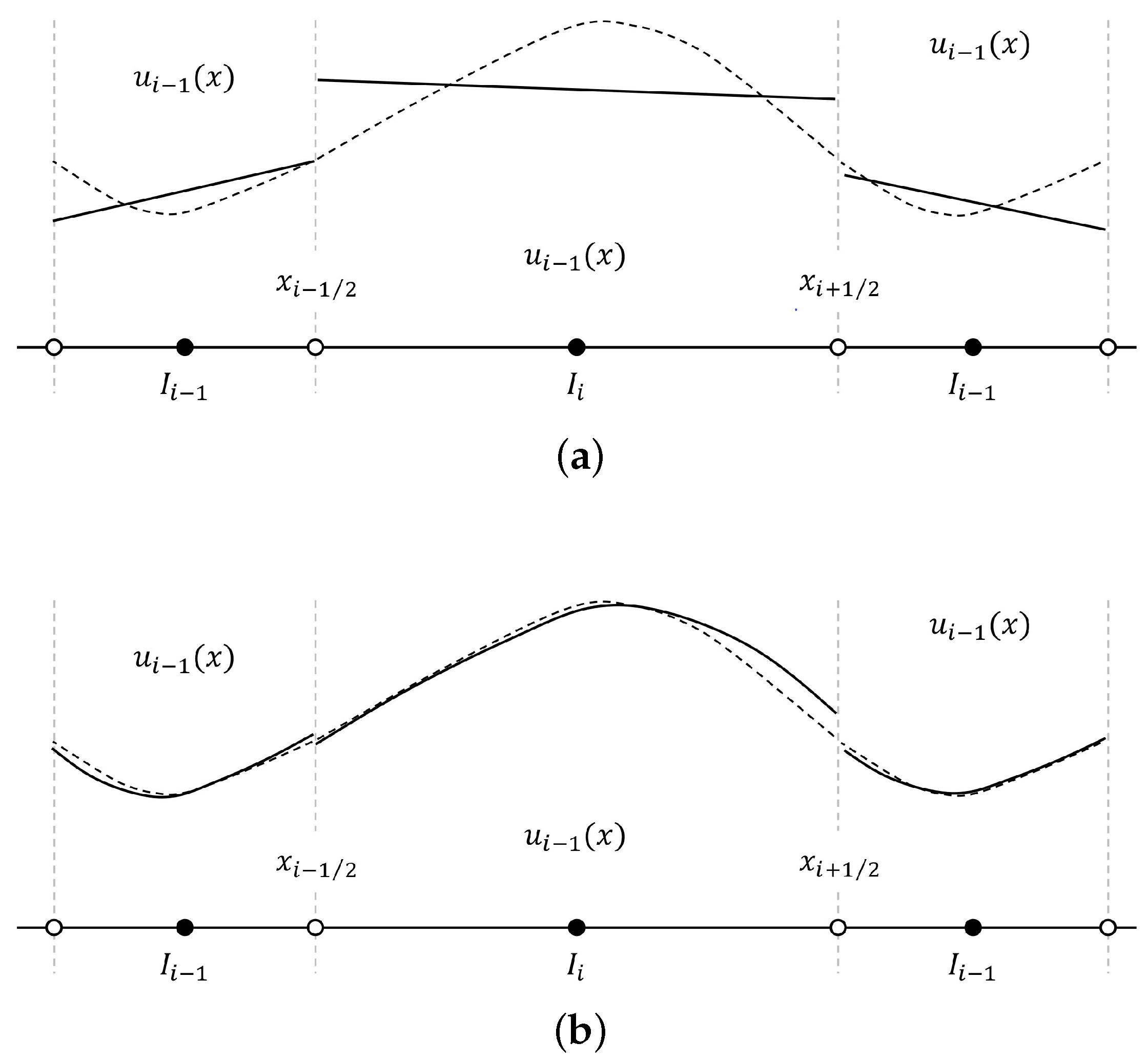
In Figure 1, within the elements, conserved quantities are represented using degree p piecewise polynomials:
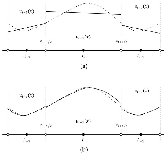
Figure 1.
Comparison of approximate solutions (solid lines) and exact solutions (dashed lines): (a) piecewise polynomials of degree ; (b) piecewise polynomials of degree .
The nondimensional Taylor basis functions can be found in [23]. The coefficients of the solution polynomials can be determined through a variational reconstruction. The cost functions employed in this approach offer flexibility, and the specific cost function utilized in this article is defined as follows:
where is selected according to [23]. The coefficients of these polynomials are determined by solving a system of linear equations:
in which denotes the neighbor cells sharing the interfaces with the current cell. The specific forms of the matrices are as follows:
The method we utilize to solve this linear system is the symmetric Gauss–Seidel (SGS) iterative method, as follows:
To achieve third-order accuracy approximation, a sufficient number of Gauss–Legendre points are required to evaluate values related to the quadratic polynomials. For convective flux and diffusive flux in Equation (1), computation over all Gauss–Legendre points on the interfaces is needed. When solving source terms, evaluation of values at each volume Gauss–Legendre point is necessary.
Equation (1) is integrated in time according to the following:
For steady-state simulations, such as fixed wings with the ALM and rotors with the ADM, GMRES with a matrix-free LU-SGS preconditioner method [30] was used to compute . The temporal discretization employed in unsteady simulations is the second-order dual time-stepping method as presented in [31]. is computed in the pseudo-time-stepping inner iteration using the following:
In the implicit inner iteration step s, the reconstruction iteration in Equation (7) is resolved once before an inner iteration step that employs the matrix-free LU-SGS approach, as proposed in [32]. In this article, the maximum of inner iteration steps is set to 20. The coupled technology makes the convergence of reconstruction and inner iteration synchronously, which can reduce the computational cost, obviously. It provides a third-order numerical accuracy, which is consistent with the spatial discretization accuracy used in this study. For more extensive details regarding the implementation of the third-order solver, please refer to [23].
2.2. Advanced Actuator Line/Disk Modeling
Actuator line and actuator disk models were integrated with each of the two solvers for comparative analysis. In this section, we will first introduce the standard ALM and the recently developed advanced ALM. As shown in Figure 2, the former applies the volume force source terms of segmented blade elements to the control volumes using an isotropic Gaussian projection method, with the projection domain being a spherical shape. In contrast, the latter employs a linear distribution along the blade span, addressing the issue of inconsistency between the model and the actual force distribution. This inconsistency becomes particularly noticeable, especially when the density of force distribution is low at certain locations along the span, such as at the actuator points.
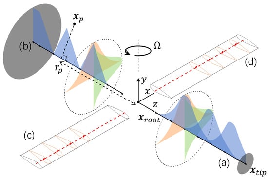
Figure 2.
Projection domain of standard actuator line model in blade (a) and advanced actuator line model in blade (b). Blade (c) and blade (d) show the blade element section discretization.
For the standard ALM, the volume force density at the center of the control volume for the mth actuator point (aerodynamic point at 1/4 chord length) on the nth blade can be represented as follows:
The projection function is denoted as follows:
Here, represents the distance between the control volume center and the actuator point. is the Gaussian length scale, and the projection function decays to of its maximum value when . Therefore, the number of control volumes corresponding to each actuator point is finite, ensuring that the computational cost required for the ALM and ADM is limited.
The projection function for the advanced ALM can be expressed as follows:
where represents the spacing between actuator points, and the distance from the center of the control volume to the actuator line of the corresponding control point on the blade can be expressed as follows:
Additionally, is defined as follows:
where . For the control volume center radial coordinates , they must satisfy . Special considerations need to be taken into account, and for the root region of the first actuator point and tip region of the last actuator point . Compared with the standard actuator line model, the projection domain of this model follows a cylindrical distribution, and the linear radial distribution is more reasonable.
To prevent numerical instability caused by insufficient grid resolution or projection function volume integrals less than the unit at the root and tip of the blades, it is necessary to normalize Equation (10), denoted as follows:
The calculation of loads on the segmented rotor blades is determined by the following:
when , it corresponds to the ALM. However, if exceeds , it corresponds to the ADM, where the right-hand term introduces a time-averaging effect. In the case of using the ADM, is typically chosen to evenly distribute the time-averaged load over the disk area. Additionally, the calculations of blade element force in Figure 3 are based on the following:
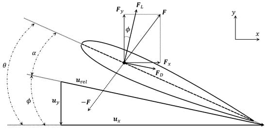
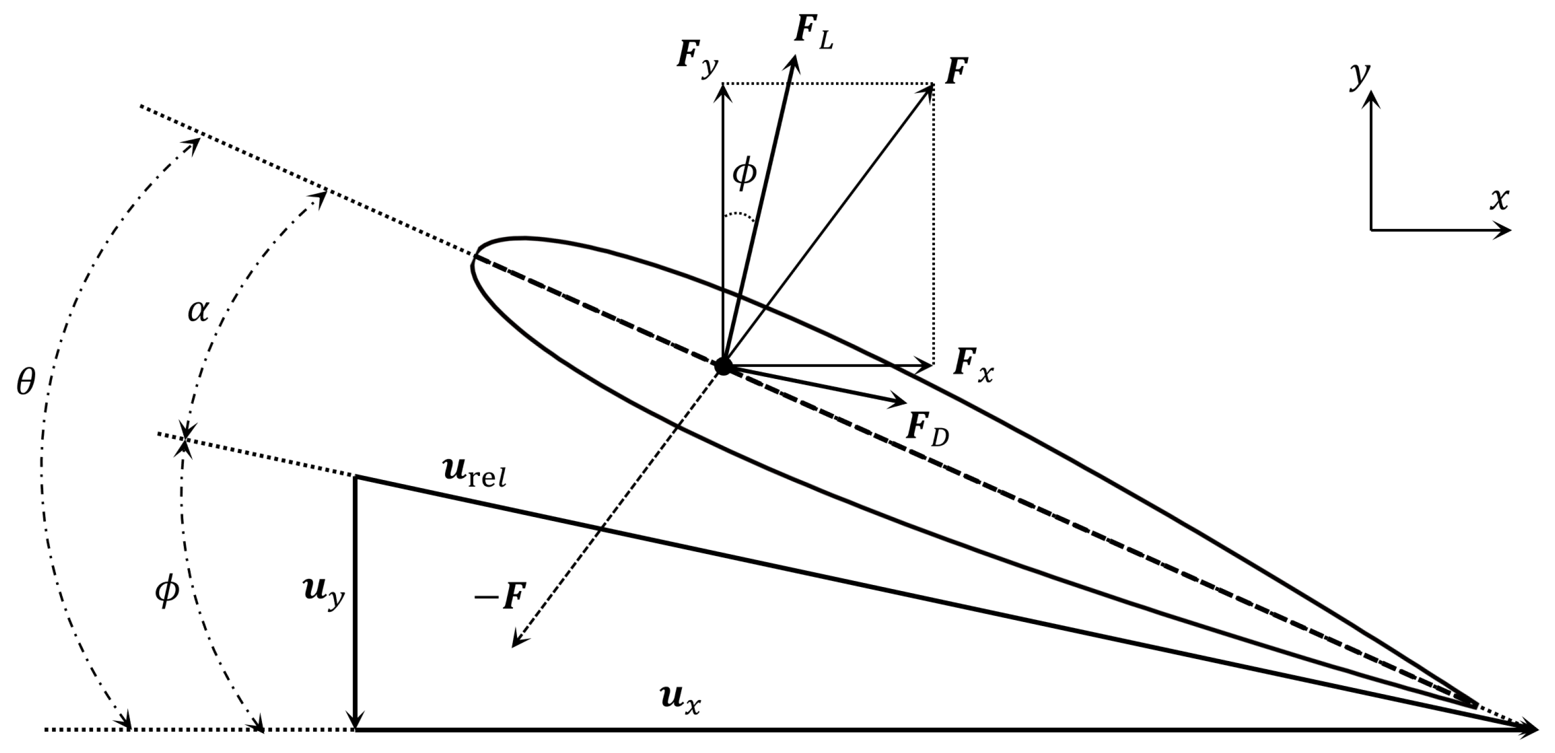
Figure 3.
Schematic diagram of a 2D blade element.
For a blade element, c is the local chord length. The lift coefficient and drag coefficient of the segmented 2D airfoil can be obtained based on experimental results and tables generated by the XFLR5 v6.59 software [33], respectively. and are the unit vectors of the local coordinate system of blades. is evaluated according to the sampled velocity and rotor motion velocity, which is required for the computation of parameters such as the angle of attack .
To yield stable and accurate sampling results, the velocity sampling method involves the weighted average of the values of cells surrounding the actuator points, utilizing a projection function denoted as follows:
2.3. Improved Tip loss Correction
In [11,19], the authors have shown that the parameter in the ALM projection function has an impact on the vortex core scale near the blade tip. While projection with can produce a reasonable vortex core scale, it required a grid size satisfying to reduce numerical error due to insufficient resolution. Consequently, it is likely to underestimate the blade tip vortex core scale for relatively coarse grids and overestimate lift coefficients. We improve the correction of the filtered ALM originally proposed by [18] and extend its application to rotor aerodynamic calculations utilizing the advanced ALM and ADM. The improved correction guarantees the accuracy of load calculation in simulations with coarse grids.
Following the approach described in [18], this article corrects the sampled velocities in the flow field. Initially, the free stream velocity is obtained by , removing the influence of the vortex core scale . The computation of the variable using the circulation and inflow velocity in the previous time step according to the following:
The finite difference of in [18] is computed using the following:
The original finite difference approach leads the overestimation of lift coefficients around the blade tip for a rotorcraft. We take the finite differences at the interfaces of sections rather than the centers and add a ghost section to keep G zero at both ends of blades, which effectively mitigates the problem of insufficient downwash velocity in the tip section correction. The improved correction using the finite difference according to the following:
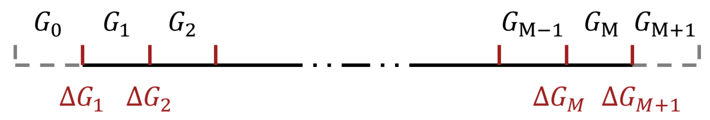
In this process, the improved differential approach is used in Figure 4, adding ghost sections at both ends, where and . The tip loss correction is employed to calculate the new downwash velocity components based on and :
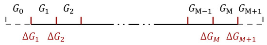
Figure 4.
Schematic diagram of the distribution of G and on a blade.
Because the solver employs a dual time-stepping inner iteration approach, the correction can be performed only once to update the downwash velocity during every pseudo time step. Through calculations, it is found that the corrected velocity computed by the following:
converges rapidly when . Since the number of actuator points is small, this method does not significantly increase the computational cost.
As mentioned in [11,19], the Gaussian length scale needs to satisfy in Equation (12) to offer accurate projections of the tip vortex size and the associated downwash, resulting in accurate predictions of the tip losses. When the mesh resolution required to resolve the vortex structure cannot be satisfied, a larger Gaussian length scale has to be employed for projection and increase the tip vortex size around the blade tips, thus underestimating the downwash velocity. This correction can be used to obtain the desired downwash velocity. is the actual Gaussian length scale used for projection in Equation (12), and is the optimal Gaussian length scale used in tip loss correction. Furthermore, we attempted to apply this correction method to the ADM, but as those adopted in the ALM is not suitable for the ADM. The tip vortex cannot be resolved with the ADM when , and the correction cannot work in this situation. In this paper, we used a fixed in the correction with the ADM for the cases of hover flight rotor and forward flight rotor to resolve the problem, and the results showed the effectiveness of the rule for selecting. This is due to time averaging of the loads and the unavailability of the tip vortex structure, which requires a larger to represent the flow structure around blade tips. The limitation of the correction for the ADM is that the rule for selecting lacks sufficient argumentation and requires further validation to determine its applicability to other rotorcraft problems.
2.4. Implementation
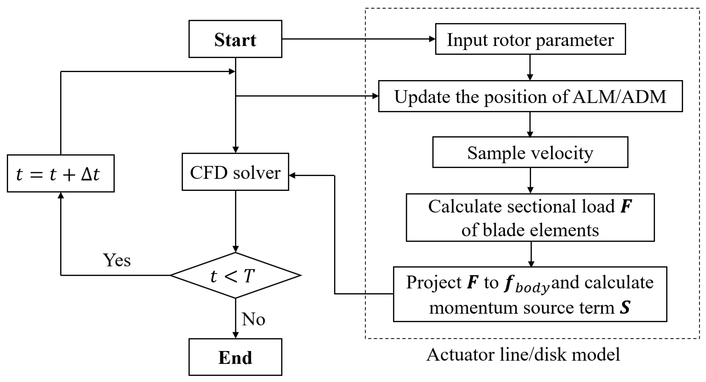
A flowchart is shown in Figure 5 to illustrate the calculation procedure, and it can be seen that the ALM/ADM module is easy to embed for CFD solvers. Algorithm 1 mentions the primary computational process of body force. At the beginning of the computation, a cylindrical subspace can be defined based on the location of the rotor, to generate a KDTree, which improves search complexity according to the control volumes in the subspace, which enhances the computational efficiency of models [8]. Unlike the ALM representing moving blades, the ADM does not require the further position of actuator points’ updates. During the correction procedure, for the ALM and for ADM. Subsequent numerical experiments demonstrate that this implementation can achieve high parallel efficiency.
| Algorithm 1: Primary computational process of body force |
| t ← t + Δt; Rotate actuation lines to new position; 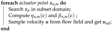 Communicate urel between processors; 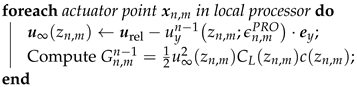 Communicate Gn−1 between processors; Compute ΔGn−1; 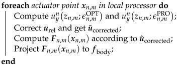 |
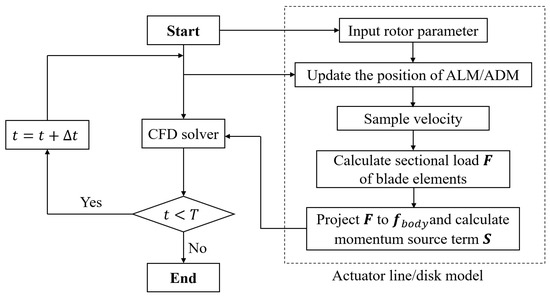
Figure 5.
Schematic flowchart of the framework of calculation.
3. Results and Discussion
3.1. Two-Dimensional Infinite Wing
To investigate the numerical convergence properties of the actuator line model and to determine the appropriate Gaussian length scale with respect to the mesh size relative to the blade chord length c, tests were conducted to simulate a two-dimensional infinite wing using the momentum source according to the following:
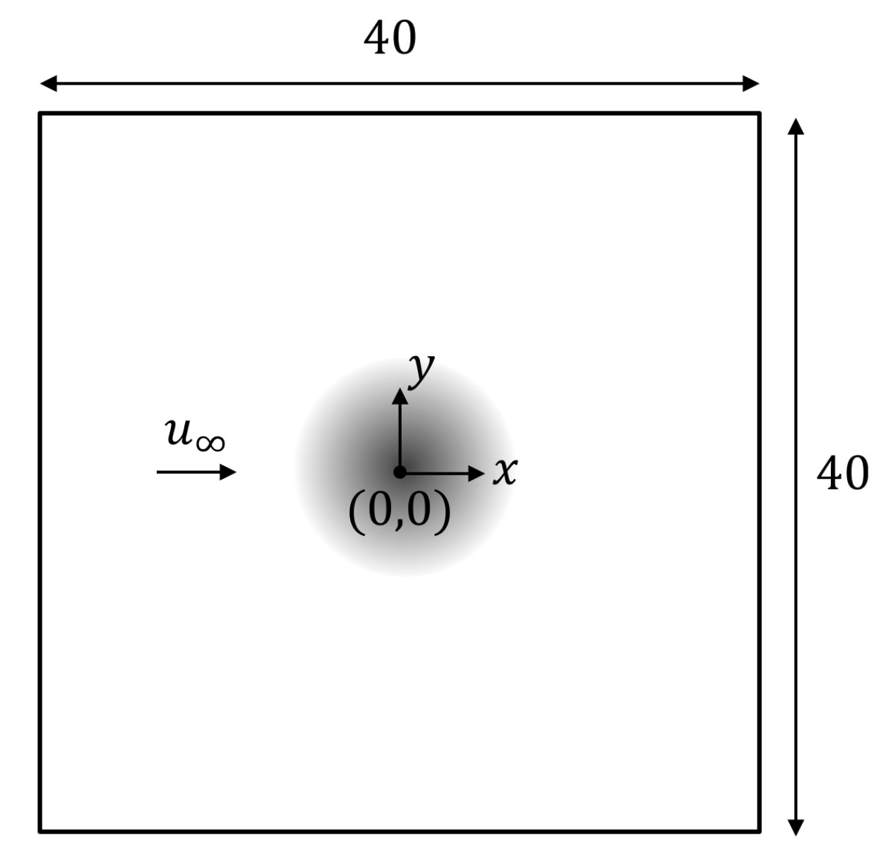
where represents the free-stream Mach number, and is the chord. The drag of the wing in the x-direction was not taken into account. We specified to calculate the lift in the y-direction to exclude the effects of sampling errors. When a momentum source was added to the flow field, the velocity gradient was high at the center of the vortex, which was the major source of error in numerical simulations. The computational domain is shown in Figure 6, and different mesh refinements were performed within a circular region of radius 3 for the simulation.

Figure 6.
Schematic diagram of the two-dimensional infinite wing.
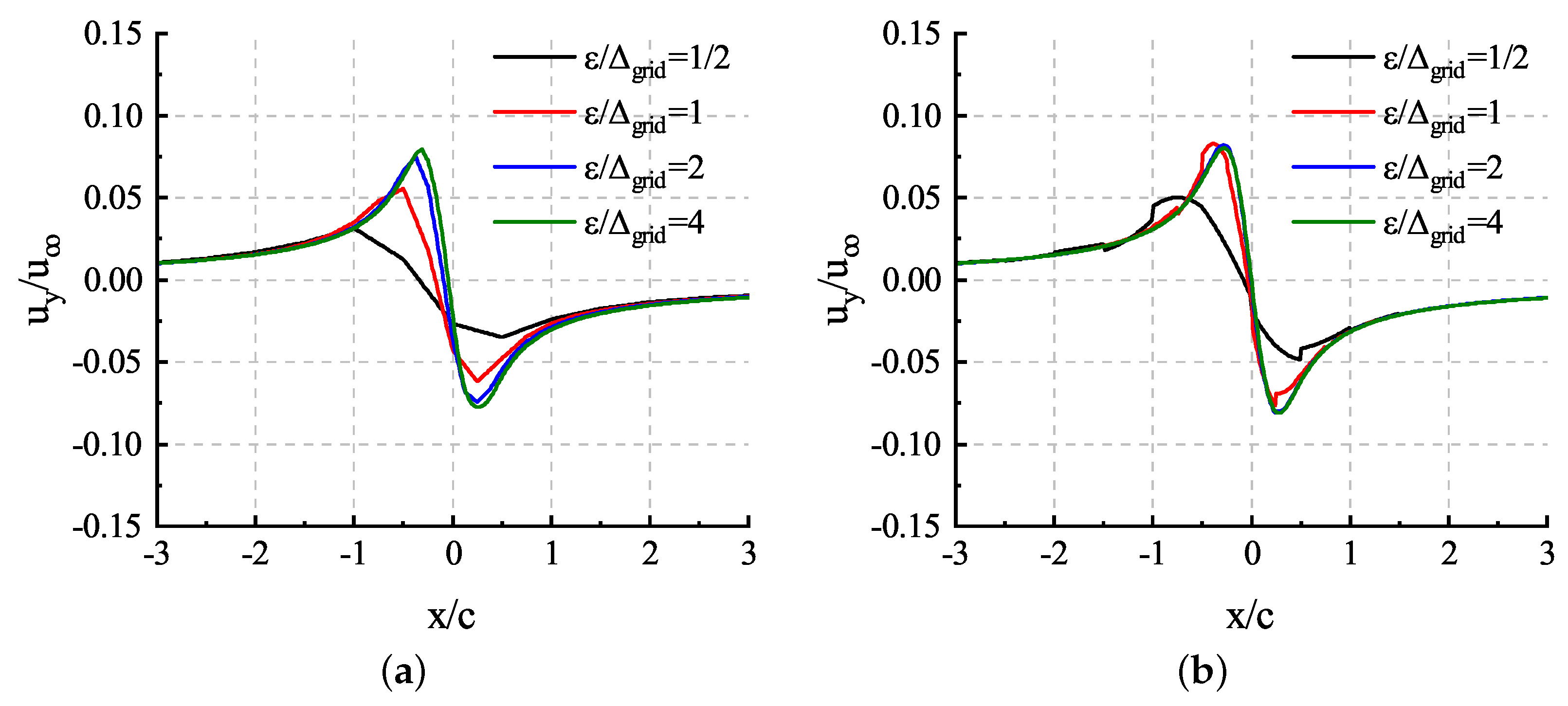
We compared the results of the third-order solver with those of the second-order solver to compare and analyze their ability to resolve the vortex structure. Consistent with the lift line method, the induced velocity should be zero at the actuator point location, i.e., the origin. According to the results in [11], the radius of the vortex core is mainly determined by , which is fixed to in this test. Through comparing the results with different grid sizes in Figure 7, we can find that the third-order solver has a stronger resolving ability for the vortex structure. To observe the difference between the numerical methods, we draw the plot with the polynomial solution inside the cell instead of just taking the average value. Compared with the results of the second-order solver relying on linear reconstruction, the third-order solver relying on the nonlinear reconstruction of the flow field can obtain convergent solutions when . With a smaller mesh size, the third-order solver has better numerical convergence. Considering that the computational cost will increase rapidly with the same grid density as the order increases, it is inevitable to reduce the grid density under the limited computational resources, which will not only weaken the advantage of the high-order method, but also result in the inability to correctly capture vortex structures in too large a grid scale. Therefore, this paper does not further increase the order of accuracy, but only adopts third-order accuracy to compare with the traditional second-order accuracy.
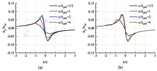
Figure 7.
Induced velocity profiles with different for 2D infinite wing: (a) results of the second−order solver; (b) results of the third−order solver.
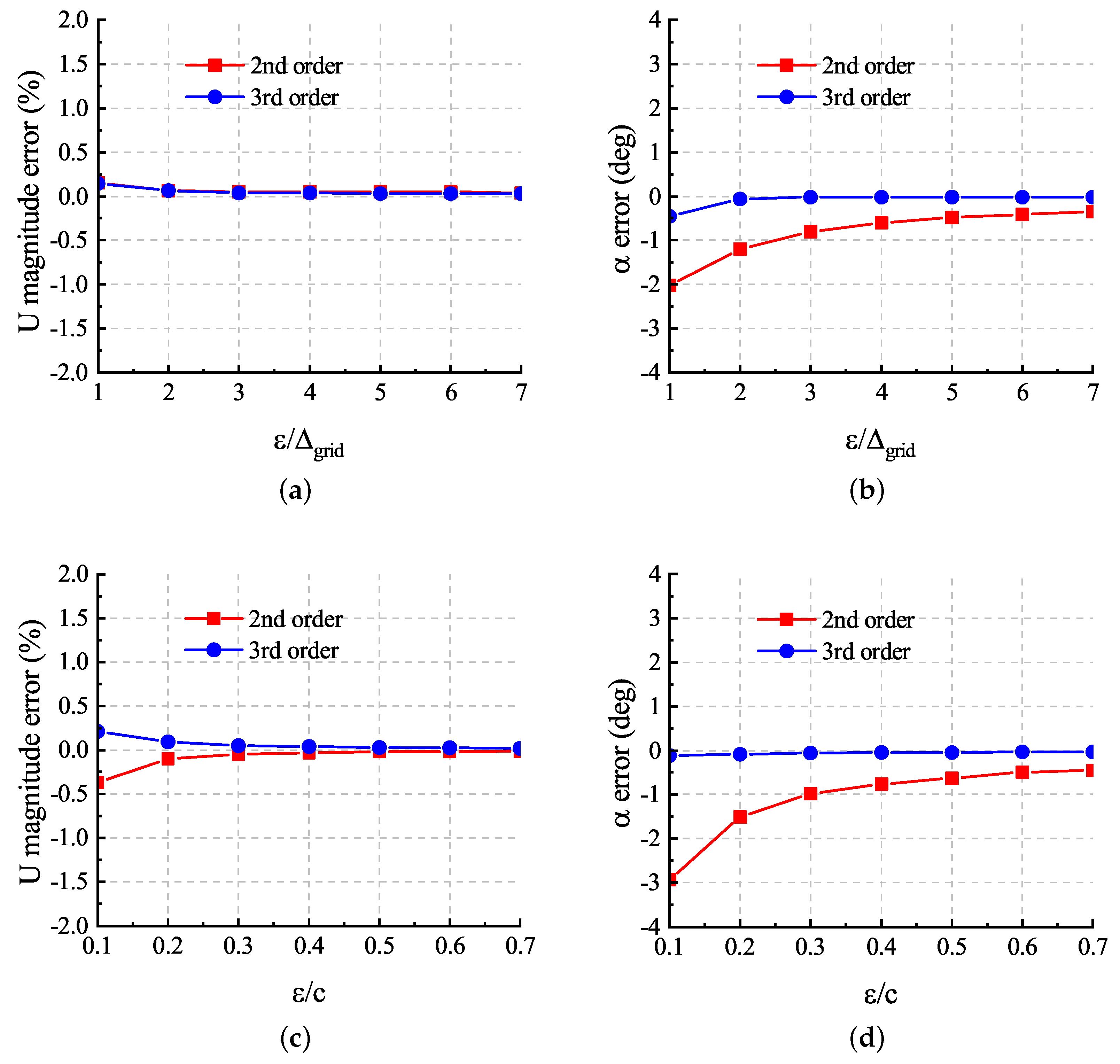
We also compared the errors of the sampled velocity at the actuator point location, mainly based on the comparison of magnitude and angle of attack. Figure 8 demonstrates that the error varies with and . The errors in the angle of attack have greater impacts on the calculation results than those in the velocity magnitude, which are only within , because the lift coefficients depend on the angle of the sampled velocity in the following cases. Compared with , had a more significant impact on errors. It is clear that the velocities obtained by the third-order solver have a smaller error because its superior vortex resolution allows for a better description of the velocity profiles shown in Figure 7. When the mesh resolution satisfies , this solver obtains the desired sampled velocity at the actuator point location.
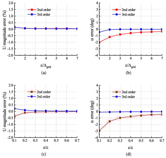
Figure 8.
Sampling error for ALM: (a) error of magnitude of velocity for different , (b) error of attack of angle for different , (c) error of magnitude of velocity for different , and (d) error of attack of angle for different .
3.2. Three-Dimensional Finite Wing
3.2.1. Constant Circulation Rectangular Wing
To investigate the relationship between the actuator line model and the lifting line theory and validate the improved tip loss correction method proposed in this paper, the case of a finite-length fixed wing with a fixed circulation distribution was designed. The rectangular wing has a chord length of with a specified lift coefficient of and a span of . The free-stream velocity . A constant circulation distribution along the span is given by .
According to the lifting line theory used in [11], we can obtain a simple theoretical solution for the induced velocity, denoted as follows:
where z is the spanwise coordinate with the wing’s center as the origin point. The vortex core radius, , is typically between and of the chord length c. In this case, we verify the consistency of the actuator line model with the lifting line approach by varying . The downwash angle can be computed by the following:
The applied source terms were the following:
Figure 9 shows the mesh used in this case, and refinement around the wing with a spacing of was performed. To preserve the numerical stability, was set according to the work in [15]. The horseshoe vortex system of the numerical solution can be observed in Figure 9. It has been shown through the research in [11] that the velocity profiles at the wing tip position are more significantly affected by than at the middle section. As the previous research practices, , mentioned in [11], yields results close to .
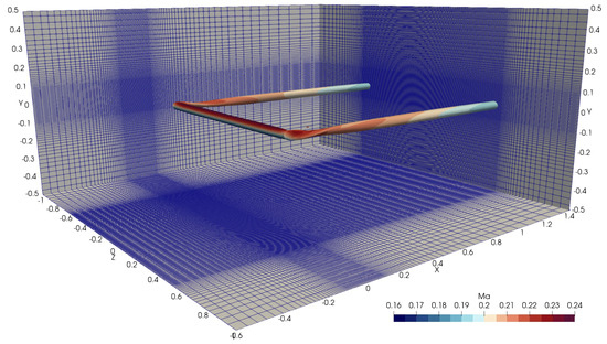
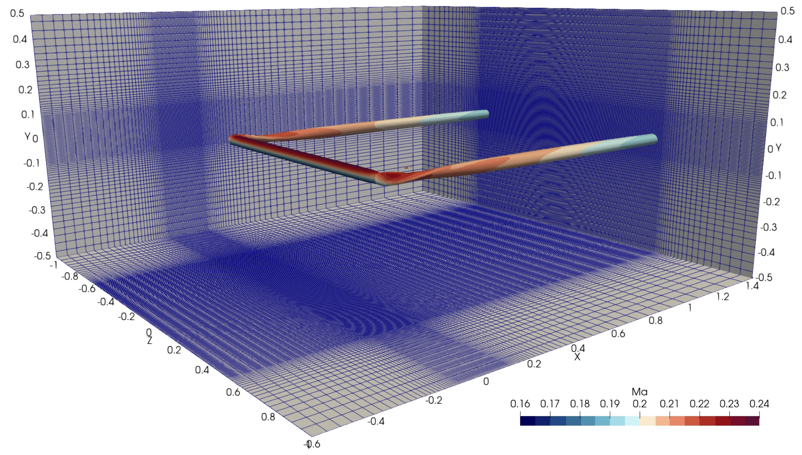
Figure 9.
Discription of the mesh for 3D finite wing and isosurface of the Q−criterion with of ALM simulation of constant circulation rectangular wing.
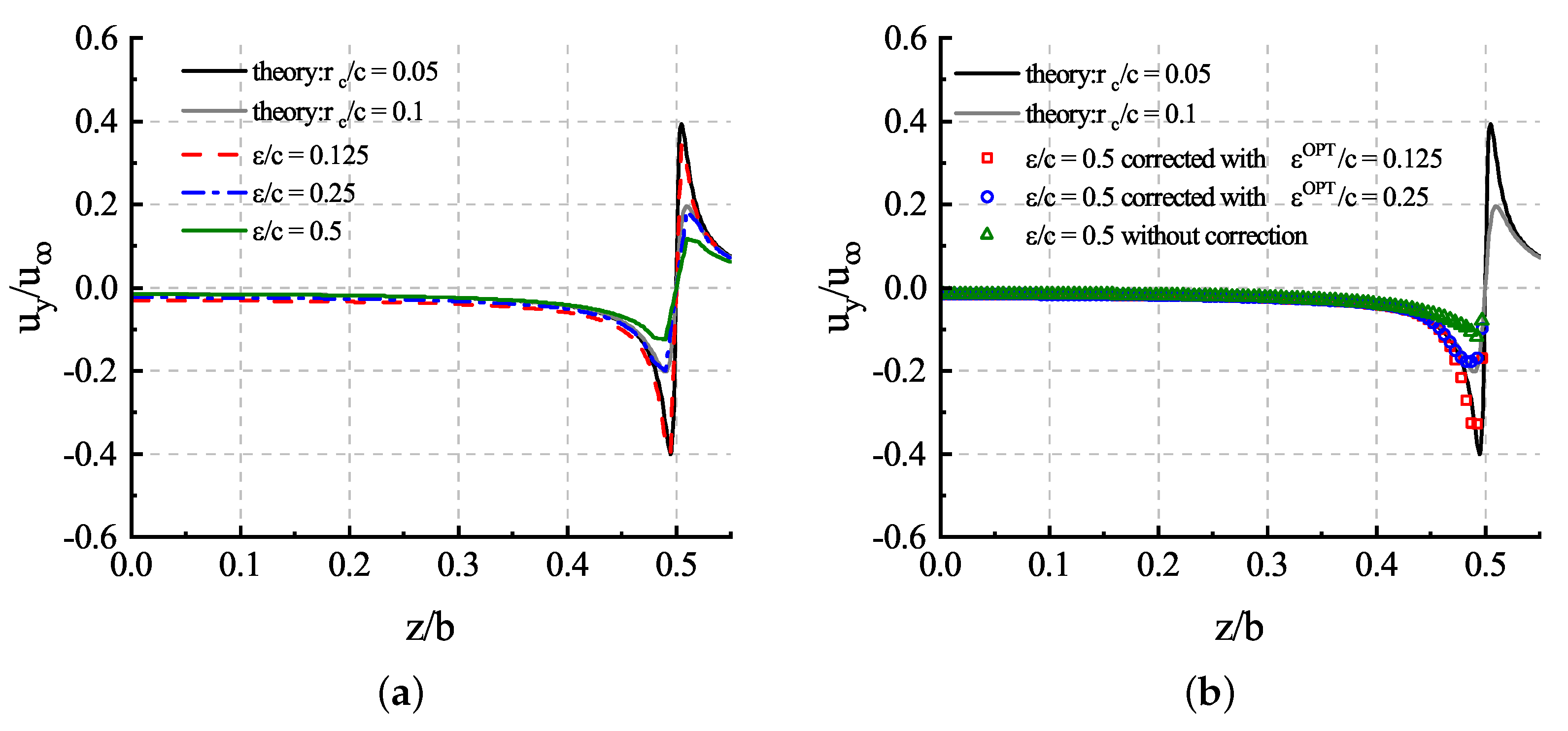
In Figure 10a, we can observe the relationship between the actuator line model and the lifting line theory by varying . The results show that the relationship between and the radius of the tip vortex core can be expressed approximately as . In addition, we fixed , and the downwash distribution corresponding to the corrected velocity can still be obtained by using the improved tip loss correction proposed in Section 2.3. It should be noted that the results in Figure 10a are obtained directly from the flow field, while in Figure 10b, the downwash results can only be obtained after correction but not directly from the flow field. The downwash velocity to be corrected is sampled from the flow field, while the corrected downwash velocity is only used to obtain the correct downwash angle for the corresponding control point, without directly affecting the flow field. The indirect effect is that the corrected downwash angle is large, resulting in less lift at that point, which is reflected in the flow field as a lower downwash velocity compared with the precorrection flow field. The downwash velocity from the tip correction can only be used to assess the load at that point and cannot correct the flow field around the tip, which is an unavoidable limitation of the tip correction method.
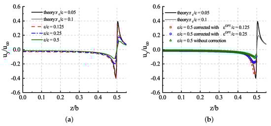
Figure 10.
Downwash distribution: (a) results of the flow field along quarter chord length position of the wing with different ; (b) results of corrected sampled velocity of the actuator line model with the same .
3.2.2. Elliptically Loaded Wing
Similar to the previous case of the rectangular wing, this case was used to investigate the relationship between the actuation line model and the lifting line theory of an elliptically loaded wing and validate the improved tip loss correction. The computational mesh for this case is the same as shown in Figure 9, with a free stream . According to analytical solutions for an elliptically loaded wing based on the lifting line theory, a constant downwash velocity along the span is represented by the following:
In this work, , the chord length distribution is as follows:
where the wingspan , and the lift coefficient of the airfoil is . The downwash angle can be computed by the following:
To obtain the theoretical solution, an angle of attack , and the angle of attack of the incoming flow . Thus, a fixed lift coefficient can be achieved.
In this case, by comparing the results of both and in Figure 11a, we can see that the chord-based gave the result closer to the theoretical solution, which is consistent with the findings in [11]. However, the chord length narrows to zero near the tip, and to preserve the numerical stability, was limited. The challenge will be more serious when the mesh is coarser. is more friendly to coarse meshes, but it underestimated downwash around tips. We alleviated this problem by employing tip loss correction; i.e., we used a constant for the projection of body force and corrected the downwash distribution with to avoid overestimating the lift near the tip, as shown in Figure 11b. Moreover, the improved tip loss correction presented in this article yielded a more continuous result when contrasted with the original correction in [18], which still underestimated the downwash velocity for sections at the tip. On the other hand, also contributed to the error near the tips. Because of the elliptic distribution of chord lengths, the chord length around the wing tips shrinks to a tiny value according to Equation (29), and it was clear that, in the ends of the wing, , even with the tip loss correction, still did not solve the problem.
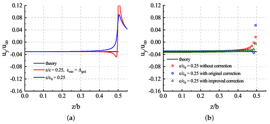
Figure 11.
Downwash distribution: (a) results of the flow field along quarter chord length position of the wing with different ; (b) results of corrected sampled velocity of the actuator line model with the same .
3.3. Hover Flight Rotor
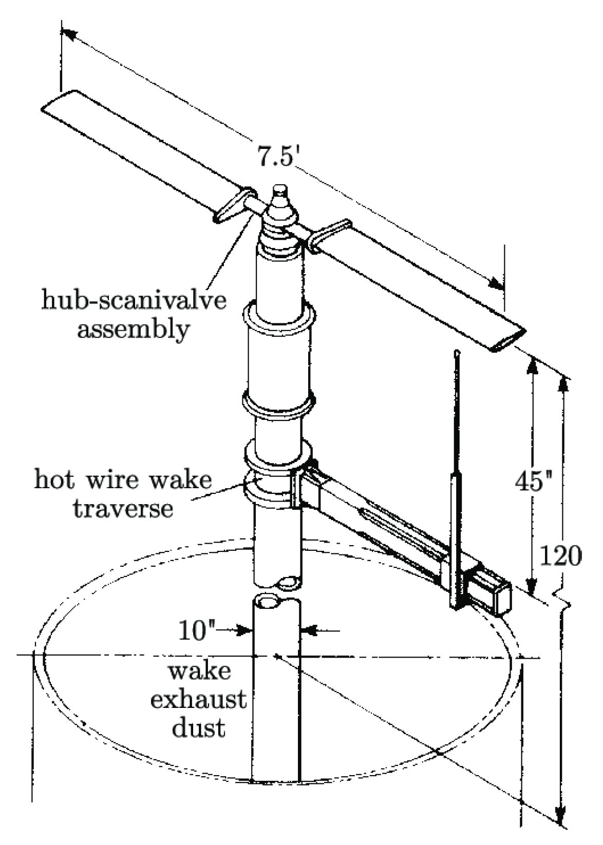
In this paper, numerical simulations of blade loads and tip vortices for a Caradonna–Tung rotor [34] were carried out for validation. According to the experiment whose device is shown in Figure 12, the rotor maximum radius m, and the aspect ratio with a chord length of m. The root cutting was . The rotor had two blades with a NACA0012 airfoil. In the simulations, the tip Mach number , and the Reynolds number . The simulations were performed for the collective pitch .
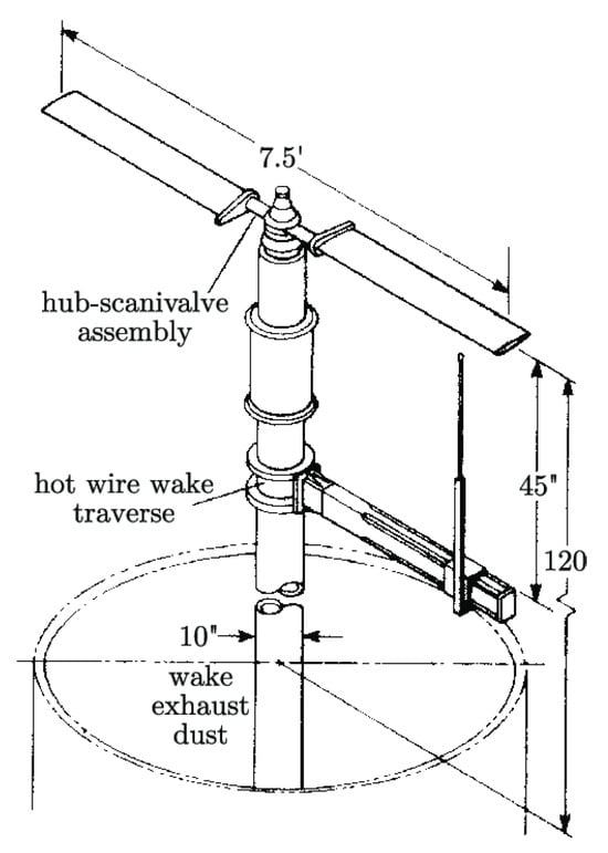
Figure 12.
Schematic diagram of Caradonna–Tung rotor experimental device [34].
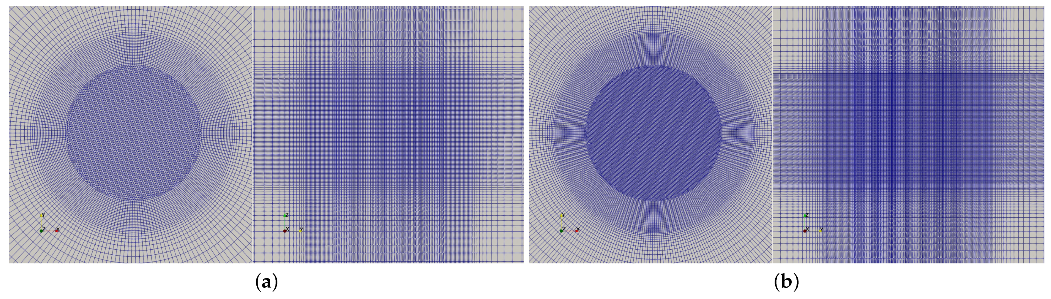
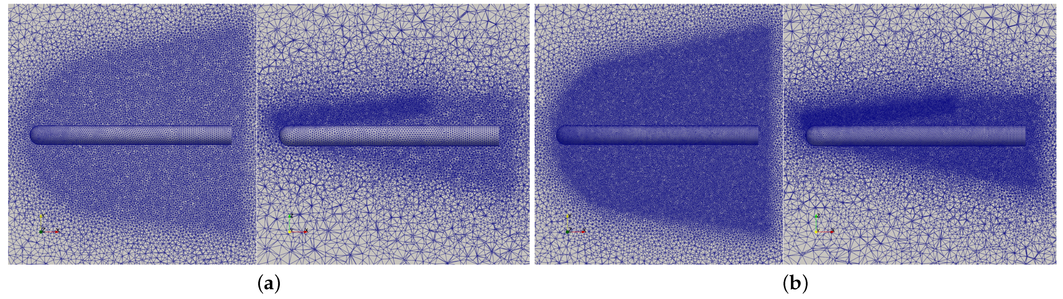
Two sets of hybrid meshes with a different refinement shown in Figure 13 were used for this simulation. The cells within the cylindrical computational domain with a radius of R are prisms, and the other domain consists of hexahedral cells. Using the field swept by the blade tips as a reference, the grid sizes in the axial, radial, and circumferential directions are shown in Table 1. The distances between the upper, lower, and radial boundaries from the rotor center were 3 R, 5 R, and 4 R. The boundary conditions of the computational domain were set to nonreflective boundary conditions, with the velocity obtained from internal cells.
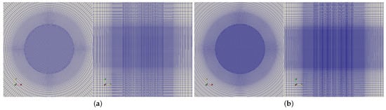
Figure 13.
The meshes used for the hover flight rotor simulation: (a) coarse mesh; (b) fine mesh.

Table 1.
Grid sizes and cell numbers of the two sets of meshes.
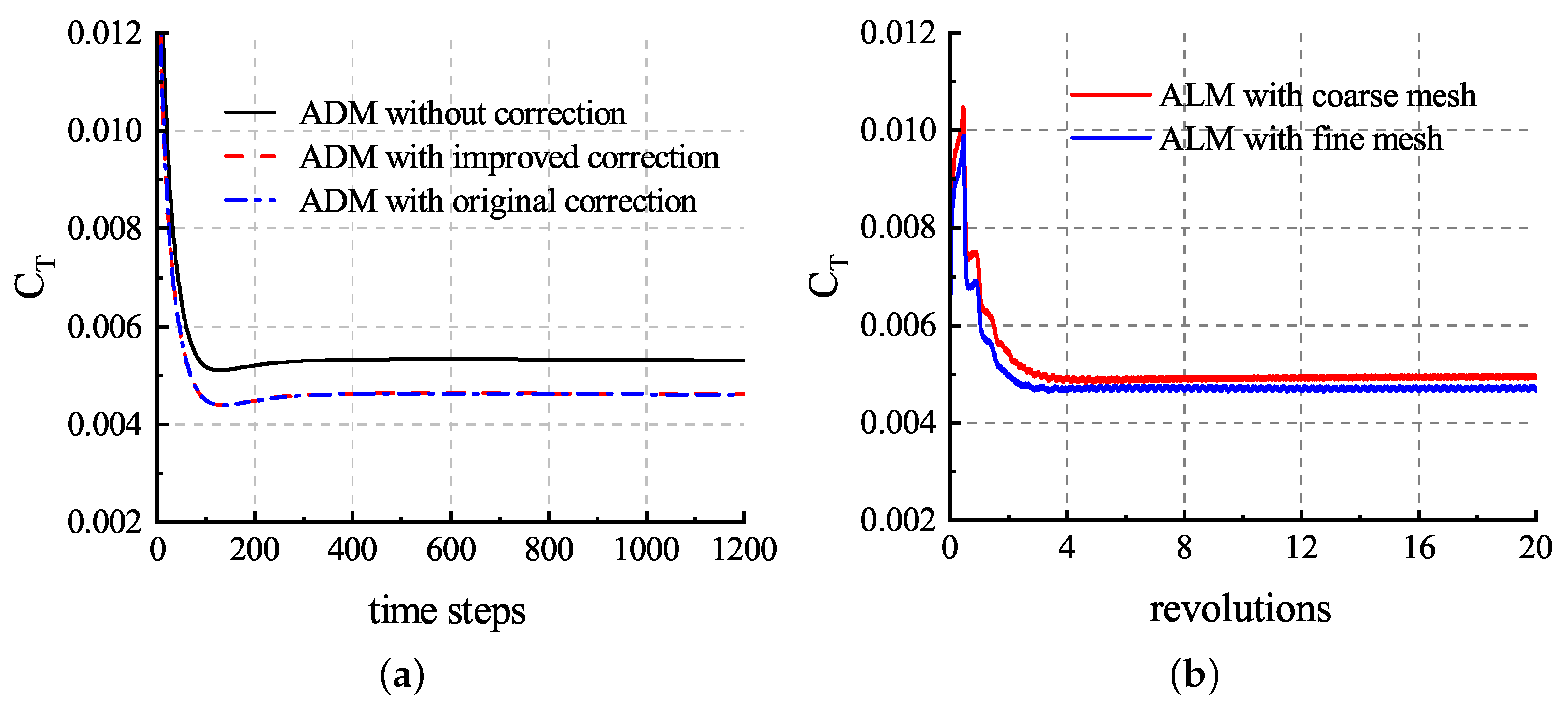
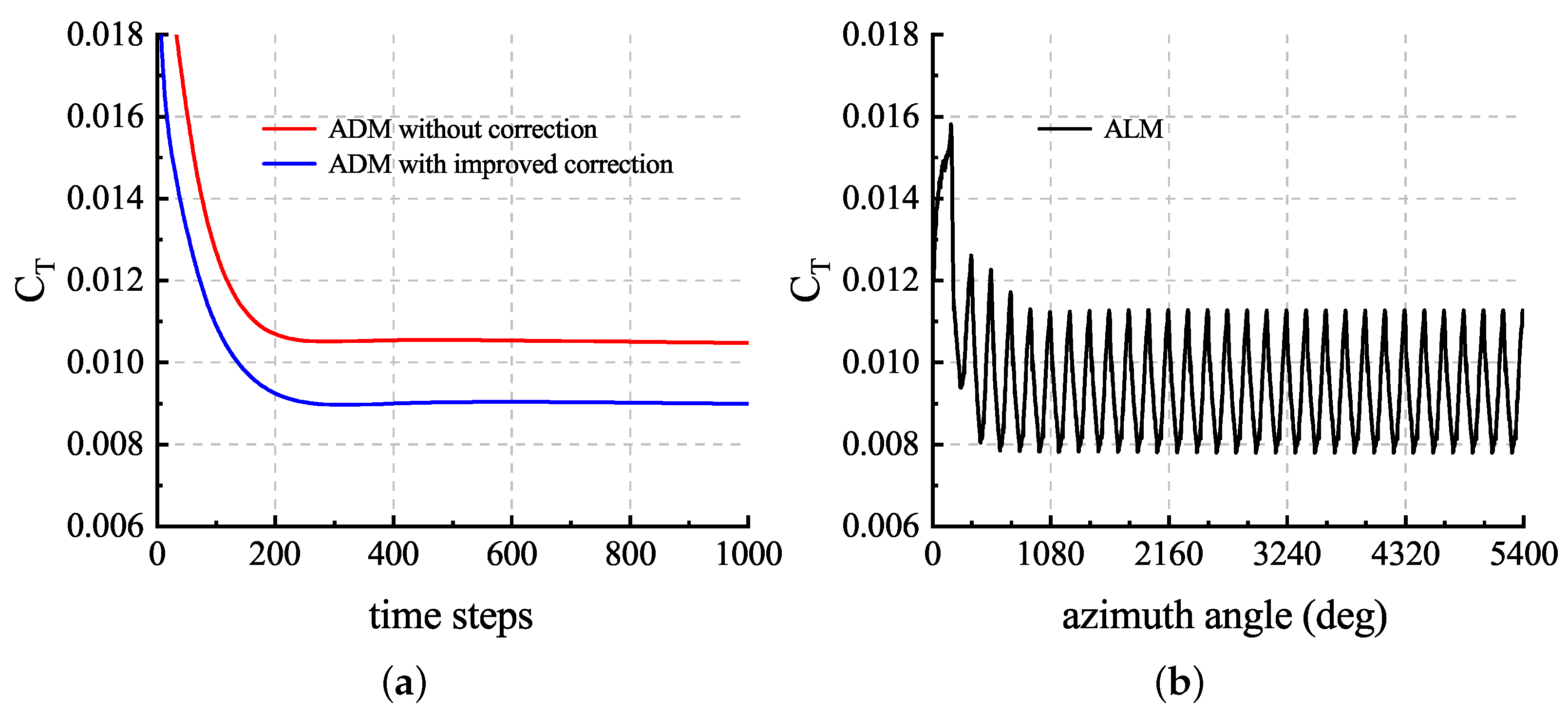
To validate the ADM and ALM, two sets of tests were performed. The first set of tests was used to compare different ADMs to simulate the hover flight rotor with the coarse mesh, and the second set of tests was the calculations using the ALM with coarse and fine meshes, respectively. According to the kinetic energy conservation approach in [35] and the experimental results, the radius of a tip vortex core is m for . Based on the relationship between and obtained in the previous section, the optimal Gaussian length scale c. For all the tests, the Gaussian length scale c and the actuator points spacing R was set. For the ADM cases, was set. As a result of time-averaging the rotor, the steady-state time-stepping method can be used to accelerate convergence, and the convergence history of the rotor thrust coefficient is shown in Figure 14a. We used a 64-core processor, and the computational time required was only about h for 1000 iteration steps. On the other hand, the calculations were carried out for 20 full revolutions, and the convergence history of the rotor thrust coefficient is shown in Figure 14b. In order to prevent numerical instability, the time step sizes need to be small enough to ensure that the blade tips move no more than one cell with adjacent time steps. As a result, the physical time steps were set equivalent to for the coarse mesh and for the fine mesh with 20 inner iterations.
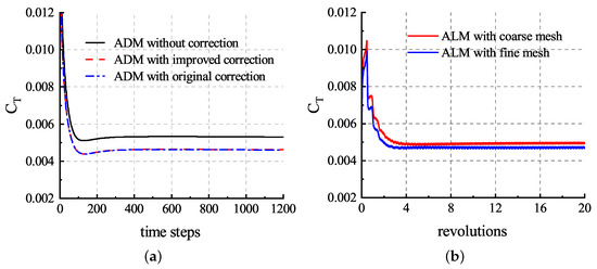
Figure 14.
Thrust coefficient convergence history of the hover flight rotor simulation: (a) results of ADM3; (b) results of ALM.
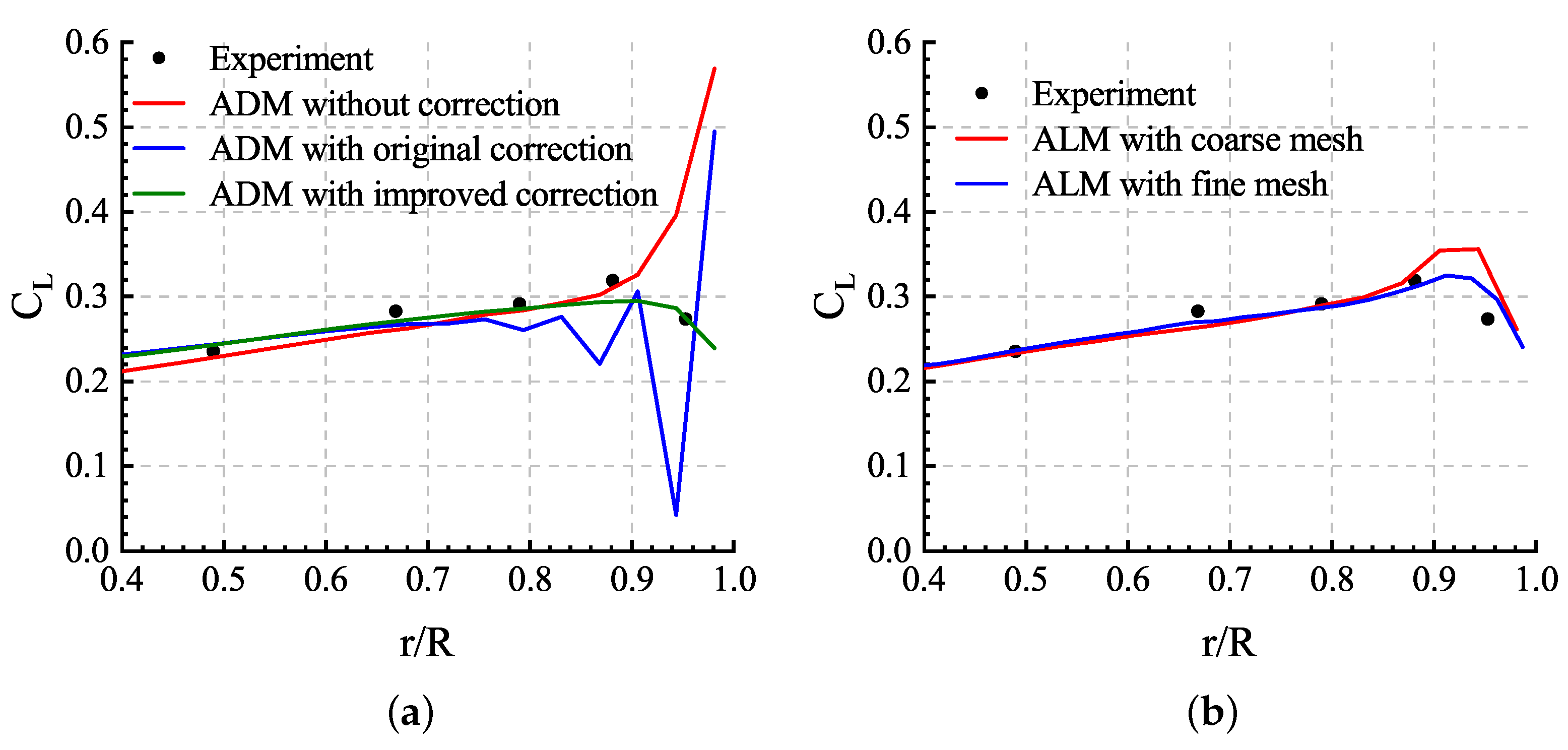
As shown in Table 2, the ADM without tip loss correction led to an overestimation of the rotor thrust coefficient. Since the ADM time-averaged the blade loads, the vortex strength near the blade tips was insufficient, thus underestimating the downwash velocity and overestimating the lift coefficient near the tips. Although the calculated rotor thrust coefficient matching the experimental value can be obtained with both of the two types of correction, as shown in Figure 15a, the sectional life coefficients were unstable near the blade tips with the original correction presented in [18], and the improved correction gave the desired results. and were adopted in the procedure of both of the tip loss corrections. On the other hand, the tip loss correction is not necessary for the ALM because the tip vortex can be captured efficiently with optimal as proposed in [13], and the results in Figure 10 proved the same. The results of the ALM in Table 2 and Figure 15b illustrate that the influence of the blade tip vortex was obtained and the tip loads were predicted correctly, especially with the fine mesh.
Table 2.
Comparison between experimental and calculation results.

Figure 15.
Sectional life coefficient distributions of the blade: (a) ADM results; (b) ALM results.
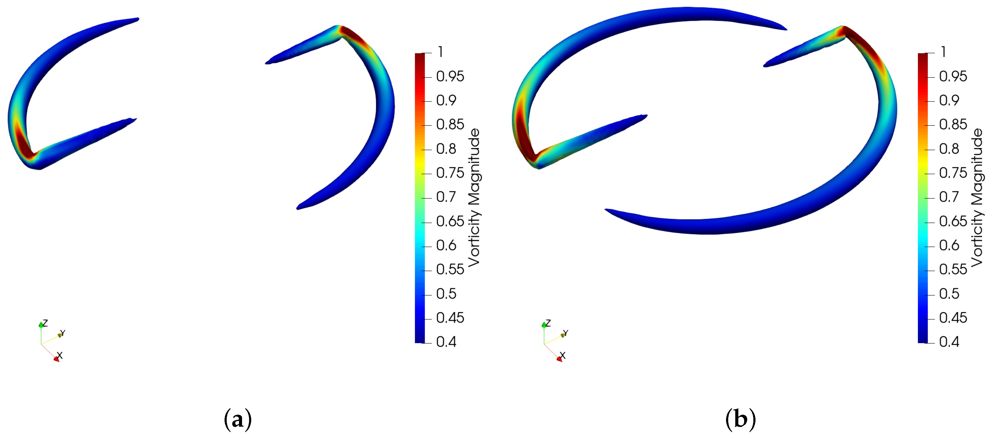
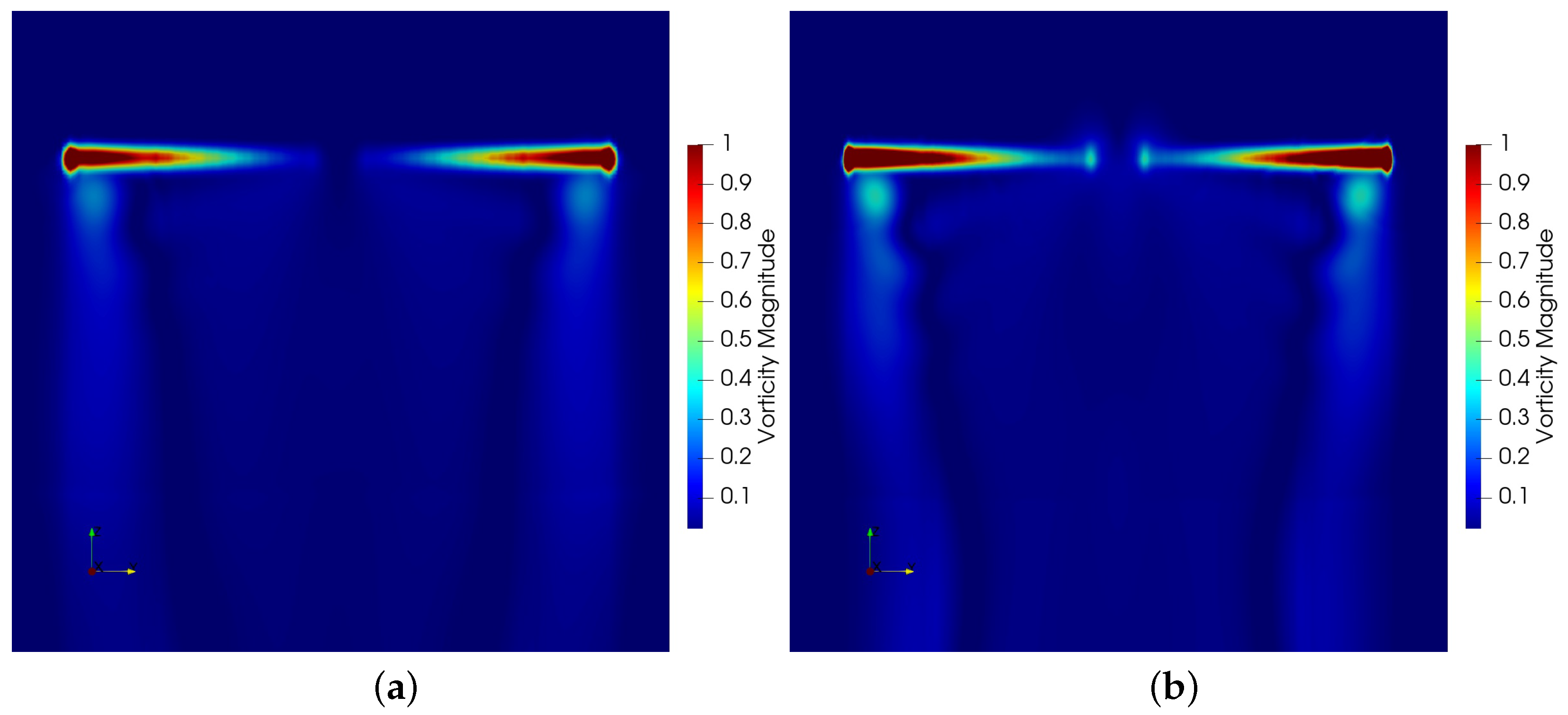
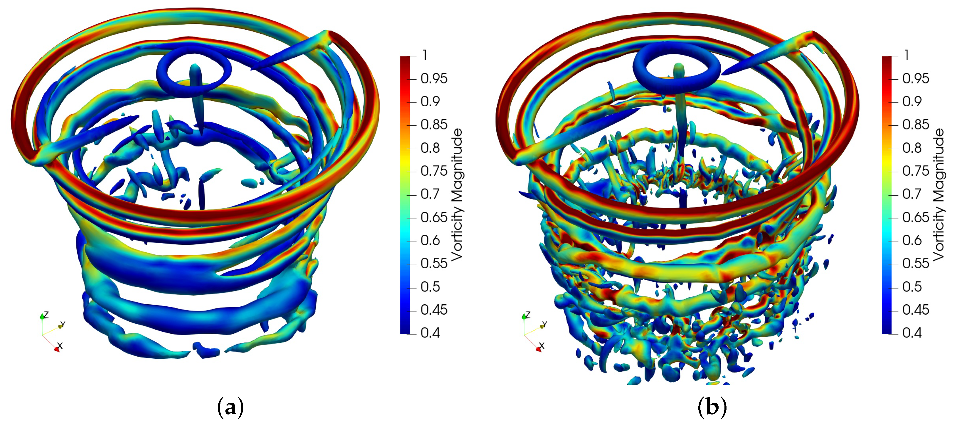
In addition, calculations with the ALM of the second-order solver were carried out. Figure 16 shows the vorticity contours at the isosurface , and Figure 17 shows the vorticity contours perpendicular to the rotor disk plane. The distinct vortex structures captured by the second-order solver only develops about a vortex age angle with the coarse mesh and about a vortex age angle with the fine mesh. The large numerical dissipation discouraged the observation of evolution progress of the expected tip vortex structures. By contrast, the ages of a vortex evolution with the third-order solver shown in Figure 18 and Figure 19 were much longer than those of the second-order counterpart.
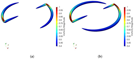
Figure 16.
Vorticity contours at isosurface of the second-order solver: (a) result with the coarse mesh; (b) result with the fine mesh.

Figure 17.
Vorticity contours of the second-order solver: (a) result with the coarse mesh; (b) result with the fine mesh.
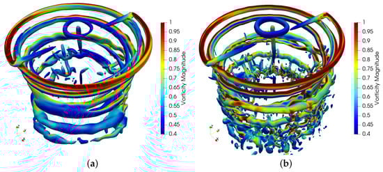
Figure 18.
Vorticity contours at isosurface of the third-order solver: (a) result with the coarse mesh; (b) result with the fine mesh.
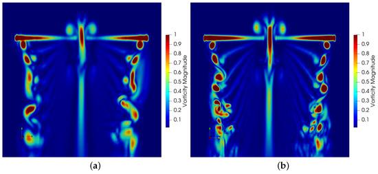
Figure 19.
Vorticity contours of the third-order solver: (a) result with the coarse mesh; (b) result with the fine mesh.
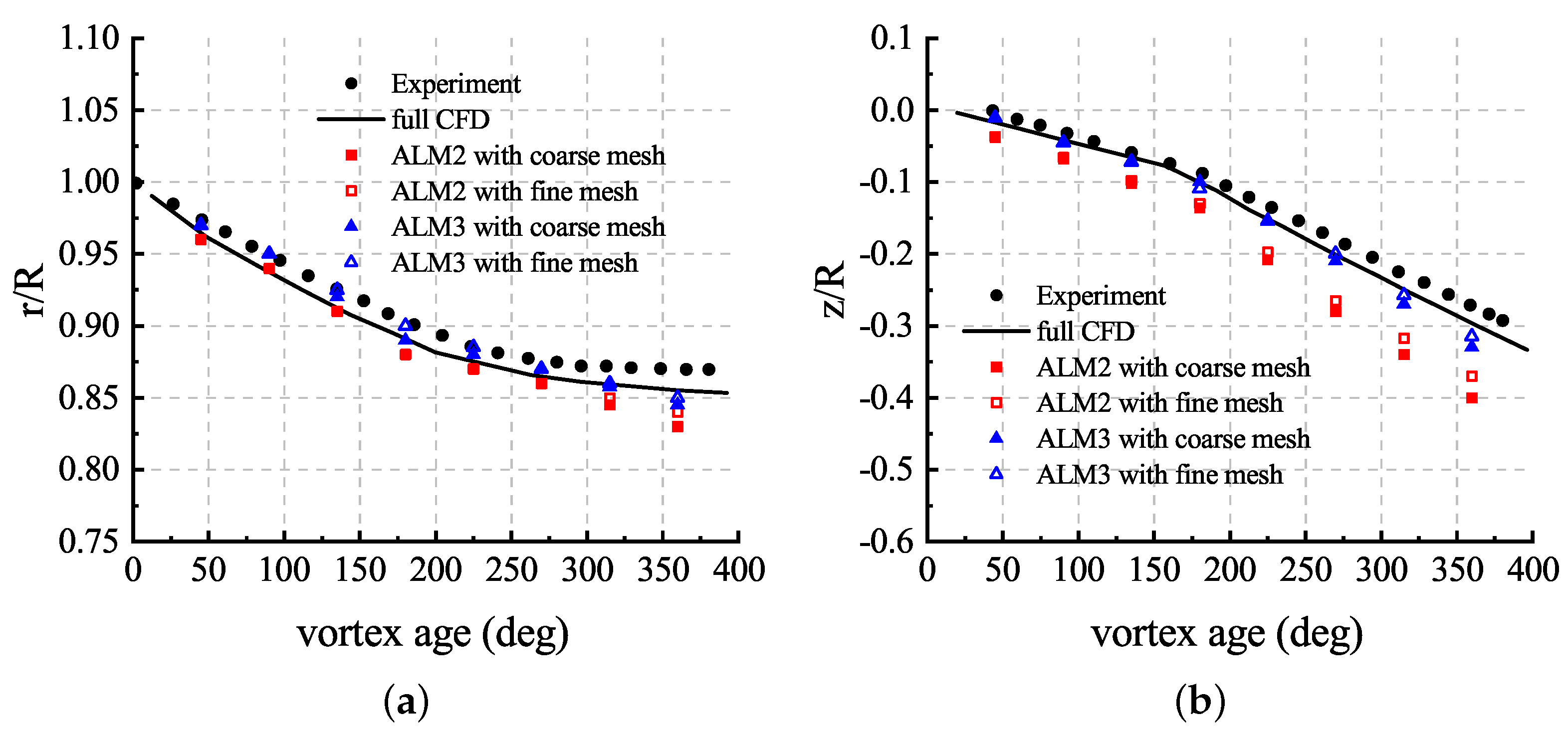
Figure 20 shows comparisons of the ALM results of blade tip vortex evolution in vertical and radial directions, where and represent the vertical position and the radial position. The full CFD results of the simulation with the RANS method based on a fifth-order WENO–Roe scheme [36] were adopted as a reference for comparison. It can be found that the ALM with the third-order solver (ALM3), due to lower numerical dissipation, predicts a better agreement with the experimental results for the vortex age up to . However, the ALM with the second-order solver (ALM2) cannot predict expected vortex core positions, and the errors mainly occur when the vortex angle exceeds . With the increase in vortex age, the vortex strength decreases. The decrease in vortex strength is caused by both physical and numerical dissipation, and the numerical dissipation plays a leading role in the simulation. Compared with the error of the radial position, a larger error can be seen in the results of the vertical position.
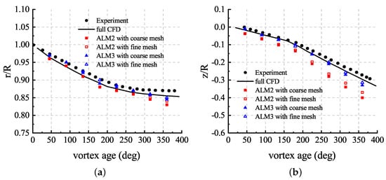
Figure 20.
Comparisons of positions of the vortex core: (a) radial position; (b) axial position.
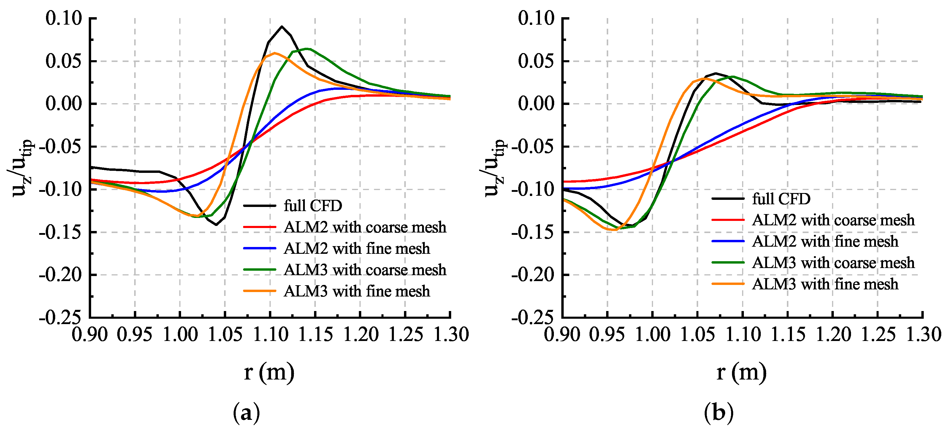
Comparisons of velocity profiles at the vortex age of and are given in Figure 21. It is clearly seen that the velocity distribution predicted by ALM3 is more reasonable using the full CFD results as a reference. With both of the coarse and fine meshes, ALM3 obtained a velocity profile much closer to the full CFD result compared with ALM2. ALM2 predicted smaller velocity peaks and a larger vortex core radius, which meant its inability to capture enough vortex strength, and refinement of a mesh cannot improve this problem effectively.
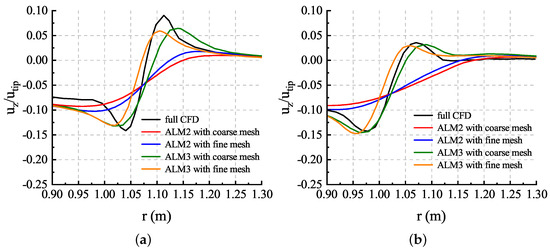
Figure 21.
Comparisons of velocity profiles: (a) velocity profiles at vortex age of ; (b) velocity profiles at vortex age of .
Table 3 shows the computational cost of ALM simulation. The core hours of simulation based on the third-order solver were about four times that of the second-order solver for the same mesh. The differentiation of reconstruction and flux calculations were the main reasons for the higher computation. However, if we consider the previous result comparisons together, ALM3 can still give better results with a coarse mesh, especially for focusing on the blade tip vortex evolution. Therefore, adopting the third-order solver is a more efficient way to capture blade tip vertices compared with the traditional second-order solver using mesh refinement.
Table 3.
Computational cost of the ALM simulation for the hover flight rotor.
3.4. Forward Flight Rotor
In the rotor–fuselage aerodynamic interaction experiment conducted at the Georgia Institute of Technology (GIT) [37], the position and tilt angle of the rotor are described in the schematic diagram of the experimental model shown in Figure 22. The rotor consisted of two rectangular blades with a radius m, and the root cutting was R. The hub was removed to simplify the model, and the simulation was performed for the collective pitch . The blades used a NACA0015 airfoil, and the chord length m. The cylinder diameter of the fuselage was m. The tip Mach number of the rotor was , and the free stream with the advance ratio . The simulations were performed using two sets of meshes with different refinements, as shown in Figure 23, and the mesh information is shown in Table 4. The slip boundary conditions were set to both the wall of the tunnel and the fuselage.
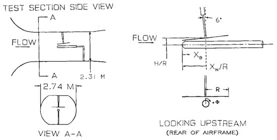
Figure 22.
Schematic diagram of the GIT experimental device [37].
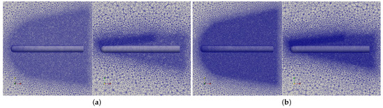
Figure 23.
The meshes used for forward flight rotor: (a) coarse mesh; (b) fine mesh.
Table 4.
Grid sizes and cell numbers of the forward flight rotor simulation.
Cases were carried out with the coarse mesh to validate the ADM and ALM. The Gaussian length scale c and actuator points spacing R were set for all the cases. For the ADM cases, was set. As a result of time-averaging the rotor, the steady-state time-stepping method can be used to accelerate convergence. The convergence history of the rotor thrust coefficient is shown in Figure 24. The of the ADM with improved correction converged to , which agreed with the experimental result of . However, the result of the ADM without correction was , which was larger than the experimental result. The calculations of the ALM without correction were carried out for 15 full revolutions, and the convergence history of the rotor thrust coefficient is shown in Figure 24b. The physical time steps were set equivalent to for the coarse mesh and for the fine mesh with 20 inner iterations. The time-averaged of the ALM was , which was slightly larger than the experimental value.
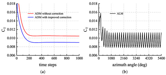
Figure 24.
Thrust coefficient convergence history of the forward flight rotor simulation: (a) ADM history; (b) ALM history.
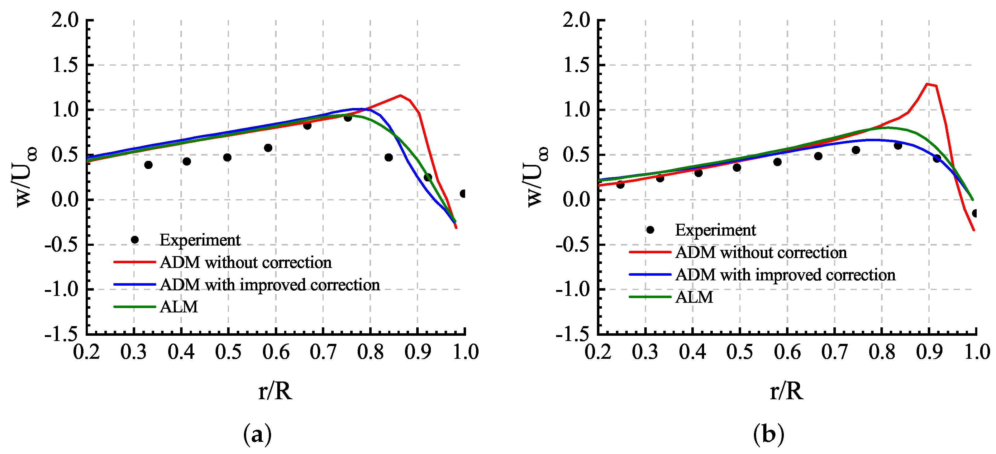
Comparisons of the time-averaged downwash velocity of the last three revolutions at different azimuth angles are shown in Figure 25. w is the velocity component directed normal to the rotor disk, and it is positive along the outflow direction. is the free-stream velocity. Similar to the situation in hover flight rotor simulation, both the ADM with improved correction and the ALM can obtain solutions agreeing with the experimental result, while the ADM without correction overestimated the downwash velocity.
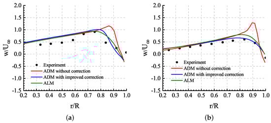
Figure 25.
Time-averaged downwash velocity along radial lines located mm below the rotor disk: (a) azimuth angle; (b) azimuth angle.
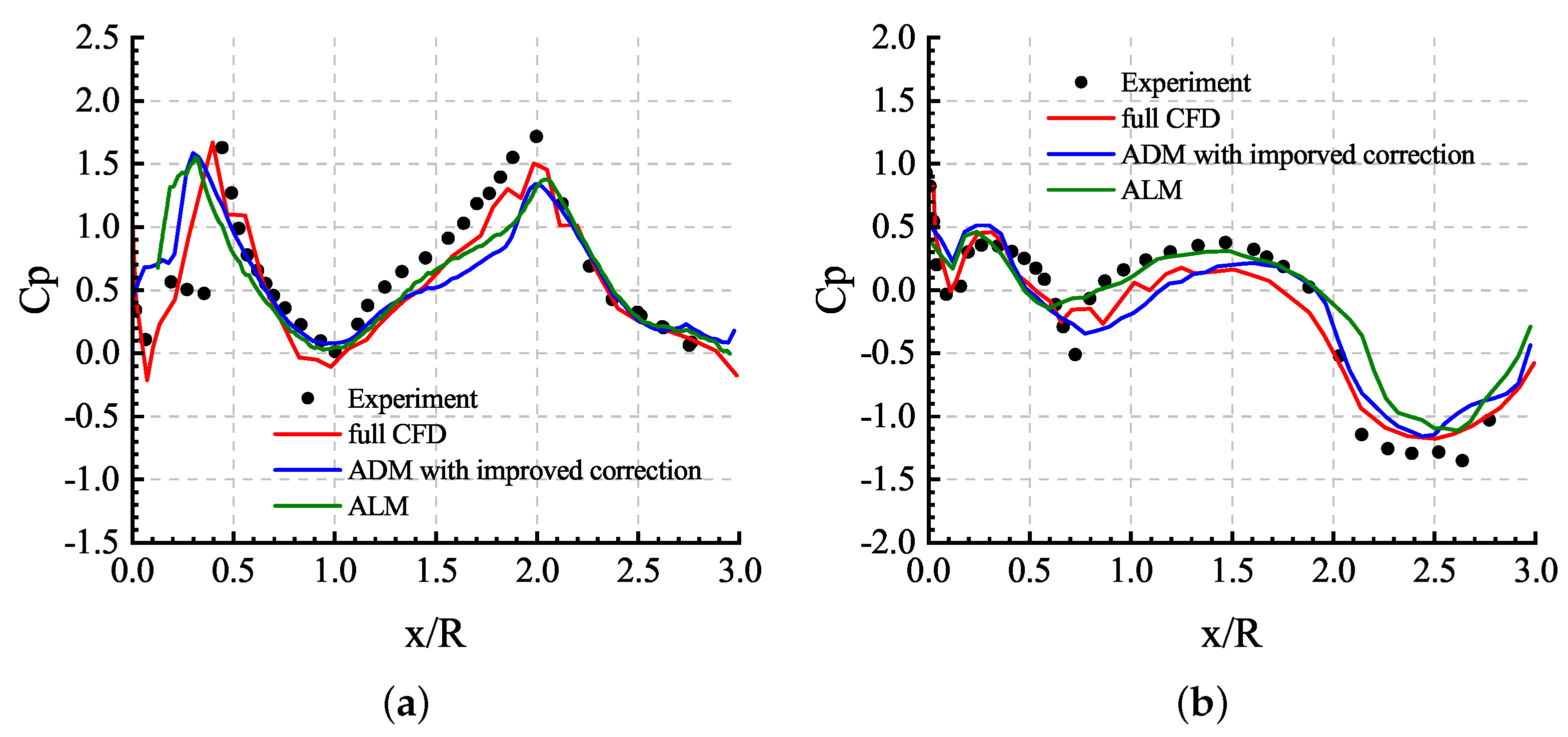
Figure 26 shows the comparisons of the time-averaged pressure coefficient of the last three revolutions on the top side () and retreating side () of the fuselage. The full CFD results are gained from [38]. Both of the ADM and ALM results agreed well with the experimental data in most of the regions. The primary error was produced on the top surface of the fuselage near the nose where the rotor disk was very close to the fuselage. The tiny distance between the blades and the fuselage led to local complex flow structures, which cannot be described by the ALM and ADM.

Figure 26.
Comparisons of time-averaged pressure coefficient on the fuselage: (a) top side; (b) retreating side.
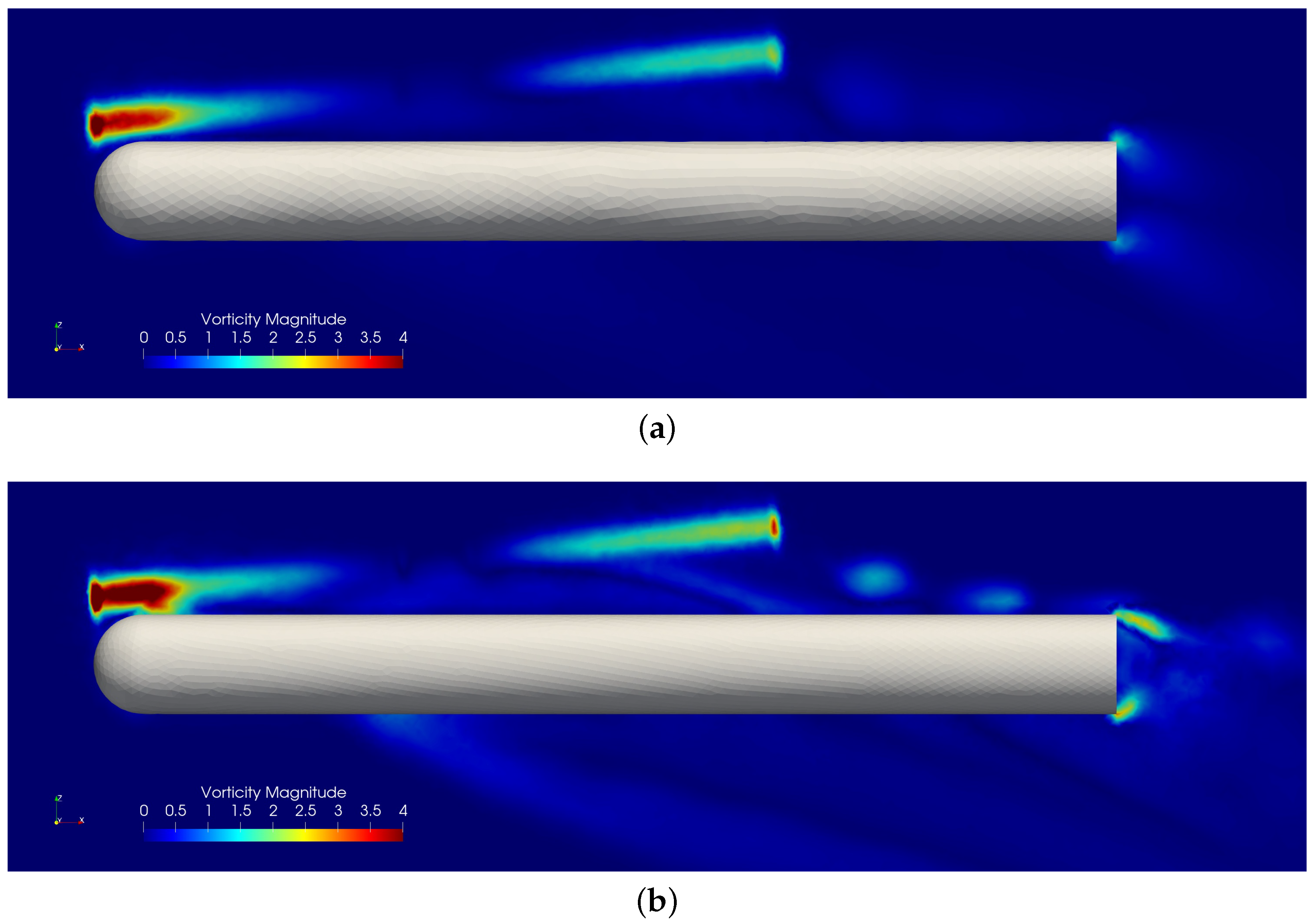
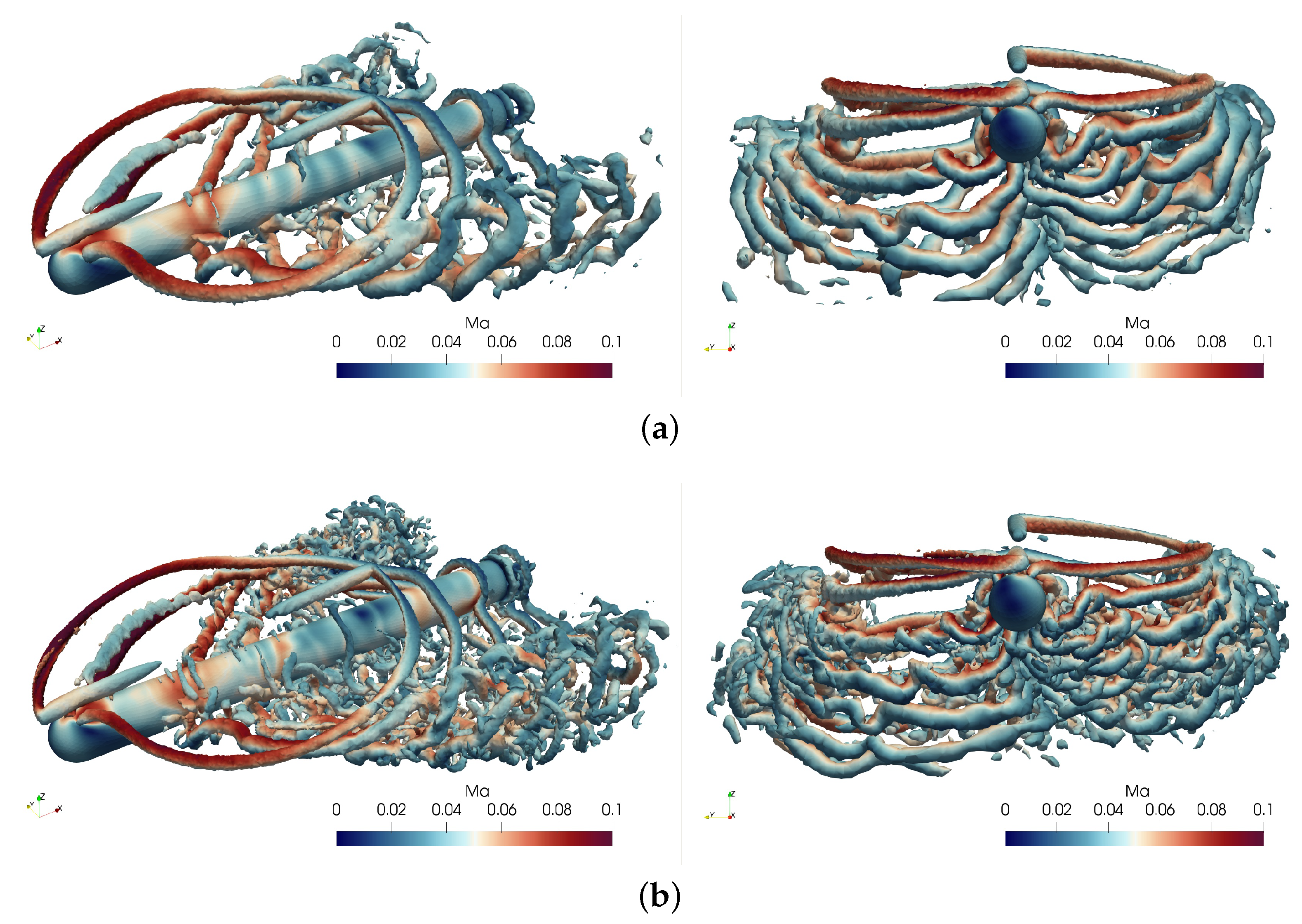
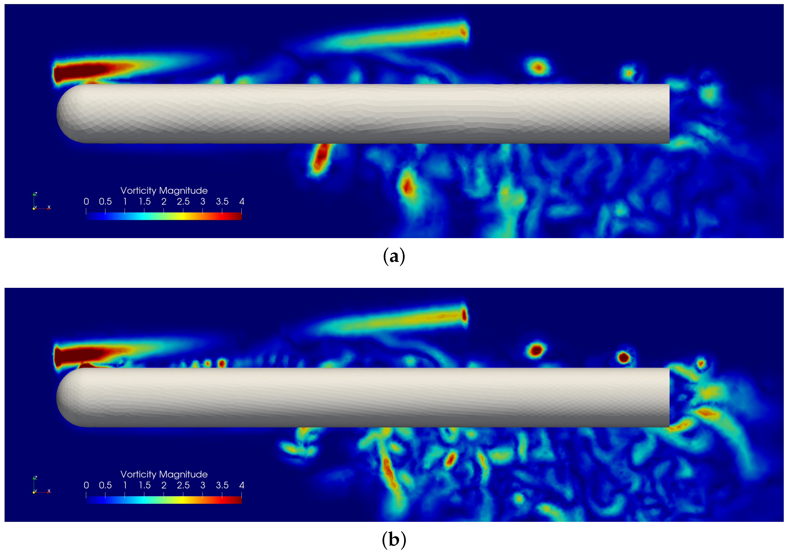
In addition, similar to the comparison in the hover flight rotor cases, calculations of the ALM with the second-order solver (ALM2) and the ALM with the third-order solver (ALM3) were carried out on both coarse and fine meshes. It can be seen form the vorticity contours at the isosurface in Figure 27 and the vorticity contours in Figure 28 that the vortex strength decreases fast in the results provided by ALM2 due to its larger numerical dissipation. By contrast, vortex structures are presented clearly with ALM3 for both the coarse and fine meshes in Figure 29 and Figure 30. The formation of the tip vortex and the position of the tip vortex as it moves back to impact the fuselage can be observed in the results of ALM3. The large-size wing tip vortex structure similar to a fixed wing produced by the rotor can also be clearly captured. Under the influence of free stream and downwash flows, the fuselage will produce a lateral velocity, and it makes the horseshoe system for greater spacing at the rear, especially at the advancing side. The features can also be observed in the results of [20]. Due to the asymmetric flow structures of the rotor blade relative to the free steam, the vortex structures on both sides of the fuselage also show obvious asymmetric characteristics, which reflects that the downwash flow on the retreating side is smaller than that on the advancing side.
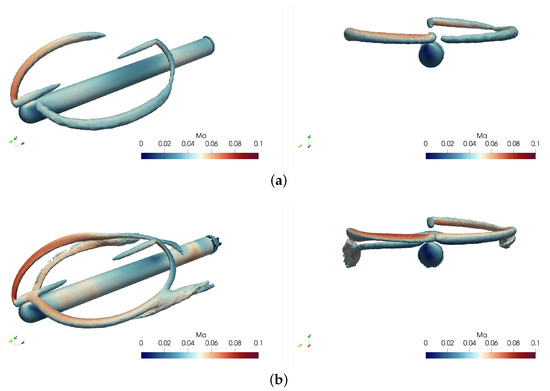
Figure 27.
Vorticity contours at isosurface of the second-order solver: (a) result with the coarse mesh; (b) result with the fine mesh.
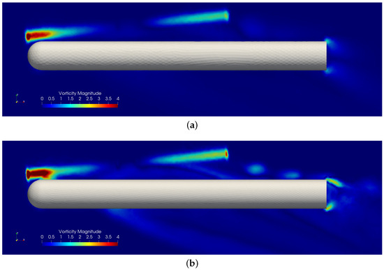
Figure 28.
Instantaneous vorticity contours at the symmetric plane of ALM2: (a) result with the coarse mesh; (b) result with the fine mesh.

Figure 29.
Vorticity contours at isosurface of the third-order solver: (a) result with the coarse mesh; (b) result with the fine mesh.
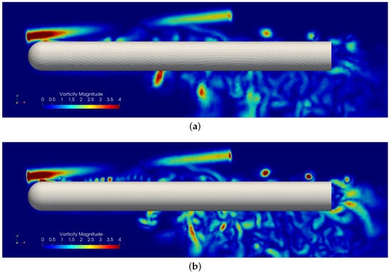
Figure 30.
Instantaneous vorticity contours at the symmetric plane of ALM3: (a) result with the coarse mesh; (b) result with the fine mesh.
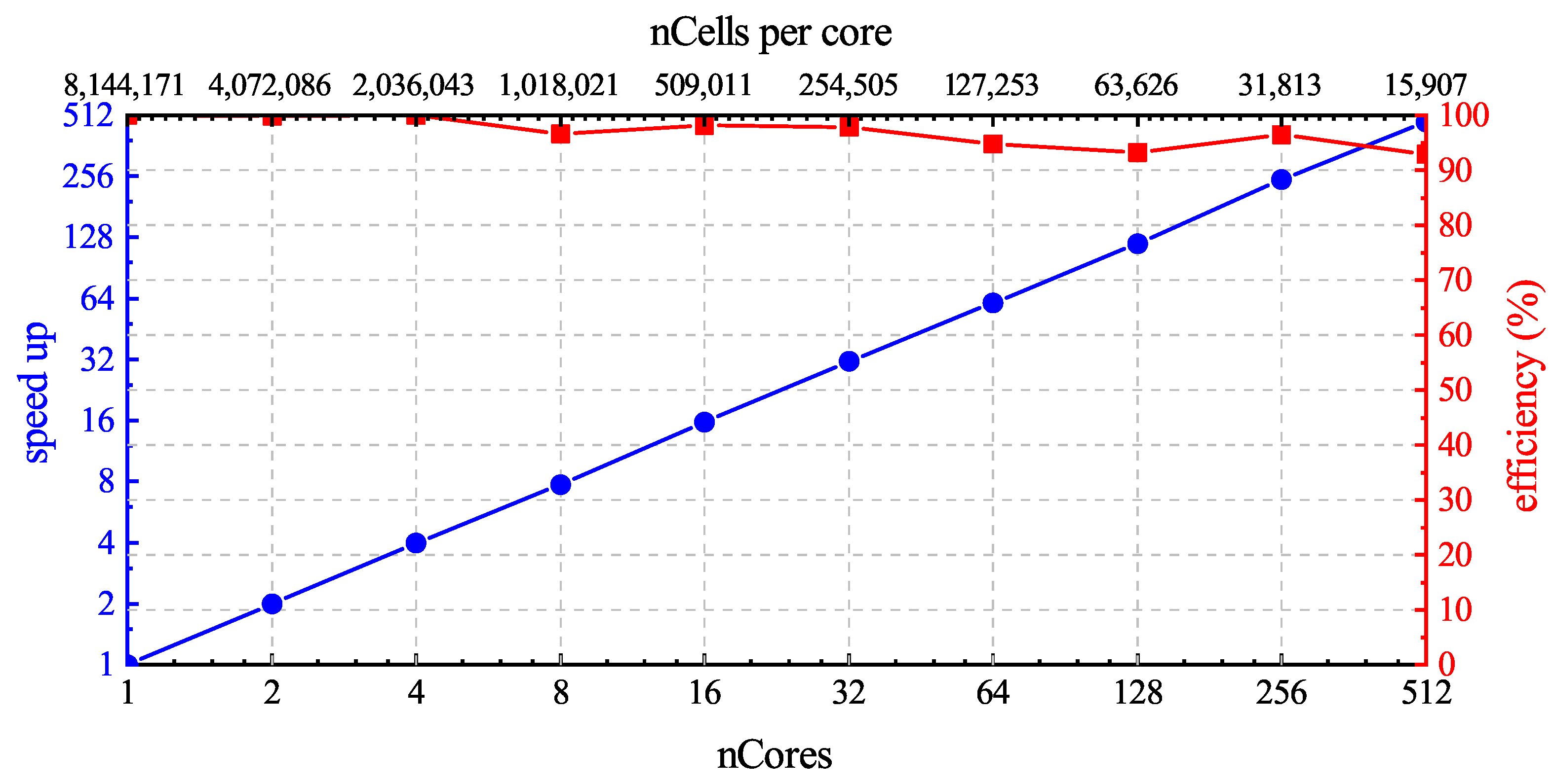
Table 5 shows the computational cost of ALM simulation. In the cases, the third-order solver provided a significant improvement in performance with about times the computational cost, compared with the second-order solver. To demonstrate the scalability of ALM3, we performed a scaling test running on the high-performance computing platform. Each computing node in the cluster comprises two Intel Xeon Gold 6240 processors, with a maximum of 32 cores per node and a maximum test core count of 512. Although the computational cost of the ALM is not equal across processors, Figure 31 illustrates the results with a parallel efficiency of up to 15,907 cells per core, which means that the ALM does not significantly reduce parallel efficiency.
Table 5.
Computational cost of the ALM simulation for the forward flight rotor.
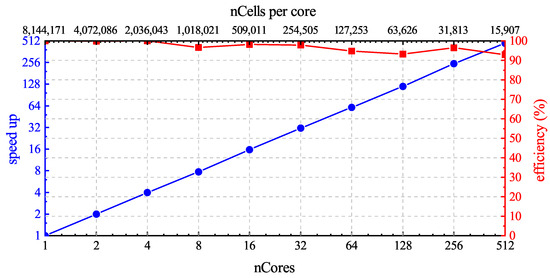
Figure 31.
Parallel scaling efficiency of the third-order solver with the ALM on the fine mesh.
4. Conclusions
In this work, we developed a combination of the advanced ALM/ADM and a third-order unstructured finite volume solver for helicopter rotors. The solver relies on implicit variational reconstruction to achieve higher-order accuracy. Unlike other higher-order solvers that require a large stencil for reconstruction, this solver only needs information from direct neighboring cells due to its compactness. Combined with the ALM/ADM for the simulation of rotors, there is no need to model a real geometric and dynamic grid, which is computationally expensive to update at each time step. The comparison of the results of the infinite wingspan tests shows that the third-order solver has better numerical convergence and smaller errors than the second-order solver for induced velocity. With the results of the fixed-wing cases, we discuss the relationship between the ALM and the lifting line theory, and validate that the downwash velocity at the wing tips can be corrected by the improved tip loss correction to obtain the theoretical solution. In the cases of the hover flight rotor and forward flight rotor, we validate the ADM and ALM, and found that the tip loss correction can help the ADM to obtain the desired downwash velocity and load around the tips through the calculation results. The performance of the third-order solver is also compared with the second-order solver on meshes with different refinements. The comparisons show that, for capturing vortex structures, it is more efficient to use the third-order solver compared with the second-order solver with mesh refinement. The results also demonstrate that the solver can be used on unstructured meshes to have high parallel efficiency and excellent scalability. Therefore, the method assists researchers in calculating blade loads and rotor-induced downwash flow with a relatively low computational cost for rotorcraft aerodynamics.
Author Contributions
Conceptualization, M.Y. and S.L.; methodology, M.Y.; software, M.Y. and W.P.; validation, M.Y. and W.P.; formal analysis, M.Y. and W.P.; investigation, M.Y. and W.P.; resources, M.Y. and W.P.; data curation, M.Y.; writing—original draft preparation, M.Y.; writing—review and editing, M.Y., W.P. and S.L.; visualization, M.Y.; supervision, W.P. and S.L.; project administration, S.L.; funding acquisition, S.L. All authors have read and agreed to the published version of the manuscript.
Funding
This research was funded by the National High-Tech R&D Program of China (863 Program), grant number 2012AA112201.
Data Availability Statement
The data presented in this article are all generated from the source code publicly available in our GitHub repository at https://github.com/buaaymh/AeroFOAM (accessed on 25 February 2024).
Acknowledgments
The authors would like to express their deepest appreciation to the high-performance computing platform provided by Beihang University.
Conflicts of Interest
The authors declare no conflicts of interest. The funders had no role in the design of the study; in the collection, analyses, or interpretation of data; in the writing of the manuscript; or in the decision to publish the results.
Abbreviations
The following abbreviations are used in this manuscript:
| ALM | actuator line model |
| ADM | actuator disk model |
| RANS | Reynolds-averaged Navier–Stokes |
| SA | Spalart–Allmaras |
| SGS | symmetric Gauss–Seidel |
| Re | Reynolds number |
| Ma | Mach number |
| body force applied on control volumes | |
| blade force of the mth section of the nth blade | |
| projection weight of blade force of the mth section of the nth blade | |
| Gaussian length scale | |
| Gaussian length scale for projection | |
| optimal Gaussian length scale | |
| grid size | |
| spacing between actuator points | |
| coordinate of control volume center | |
| coordinate of actuator point of the mth section of the nth blade | |
| coordinate of blade root | |
| coordinate of blade tip | |
| radial coordinate of control volume center | |
| radial coordinate of actuator point of the mth section of the nth blade | |
| radial coordinate of blade root | |
| radial coordinate of blade tip | |
| distance to the actuator line | |
| radial distance over spacing between actuator points | |
| volumetric normalization factor of the mth section of the nth blade | |
| blade sectional lift coefficient | |
| blade sectional drag coefficient | |
| number of blades | |
| number of actuator lines | |
| c | local chord |
| relative angle of attack of a blade section | |
| relative velocity | |
| sampled velocity | |
| corrected velocity | |
| circulation | |
| rotor thrust coefficient | |
| advance ratio |
References
- Steijl, R.; Barakos, G.; Badcock, K. A CFD framework for analysis of helicopter rotors. In Proceedings of the 17th AIAA Computational Fluid Dynamics Conference, Toronto, ON, Canada, 6–9 June 2005; p. 5124. [Google Scholar]
- Ganti, Y.; Baeder, J. CFD analysis of a slatted UH-60 rotor in hover. In Proceedings of the 30th AIAA Applied Aerodynamics Conference, New Orleans, LA, USA, 25–28 June 2012; p. 2888. [Google Scholar]
- Jain, R. Hover Predictions on the S-76 Rotor with Tip Shape Variation Using Helios. J. Aircr. 2018, 55, 66–77. [Google Scholar] [CrossRef]
- Guntupalli, K.; Rajagopalan, R.G. Development of discrete blade momentum source method for rotors in an unstructured solver. In Proceedings of the 50th AIAA Aerospace Sciences Meeting including the New Horizons Forum and Aerospace Exposition, Nashville, TN, USA, 9–12 January 2012; p. 422. [Google Scholar]
- Mikkelsen, R.F. Actuator Disc Methods Applied to Wind Turbines. Ph.D. Thesis, Technical University of Denmark, Kongens Lyngby, Denmark, 2003. [Google Scholar]
- Martinez, L.; Leonardi, S.; Churchfield, M.; Moriarty, P. A comparison of actuator disk and actuator line wind turbine models and best practices for their use. In Proceedings of the 50th AIAA Aerospace Sciences Meeting including the New Horizons Forum and Aerospace Exposition, Nashville, TN, USA, 9–12 January 2012; p. 900. [Google Scholar]
- Viguera Leza, D. Development of a Blade Element Method for CFD Simulations of Helicopter Rotors Using the Actuator Disk Approach. Master’s Thesis, Delft University of Technology, Delft, The Netherlands, 2018. [Google Scholar]
- Oruc, I.; Shenoy, R.; Shipman, J.; Horn, J.F. Towards Real-Time Fully Coupled Flight Dynamics and CFD Simulations of the Helicopter-Ship Dynamic Interface. In Proceedings of the AHS 72nd Annual Forum, West Palm, FL, USA, 17–19 May 2016. [Google Scholar]
- Shi, Y.; Xu, Y.; Zong, K.; Xu, G. An investigation of coupling ship/rotor flowfield using steady and unsteady rotor methods. Eng. Appl. Comput. Fluid Mech. 2017, 11, 417–434. [Google Scholar] [CrossRef]
- Dingxuan, Z.; Haojie, Y.; Shuangji, Y.; Tao, N. Numerical investigation for coupled rotor/ship flowfield using two models based on the momentum source method. Eng. Appl. Comput. Fluid Mech. 2021, 15, 1902–1918. [Google Scholar] [CrossRef]
- Shives, M.; Crawford, C. Mesh and load distribution requirements for actuator line CFD simulations. Wind. Energy 2013, 16, 1183–1196. [Google Scholar] [CrossRef]
- Jha, P.K.; Schmitz, S. Actuator curve embedding–An advanced actuator line model. J. Fluid Mech. 2018, 834, R2. [Google Scholar] [CrossRef]
- Churchfield, M.J.; Schreck, S.J.; Martinez, L.A.; Meneveau, C.; Spalart, P.R. An advanced actuator line method for wind energy applications and beyond. In Proceedings of the 35th Wind Energy Symposium, Grapevine, TX, USA, 9–13 January 2017; p. 1998. [Google Scholar]
- Shen, W.Z.; Mikkelsen, R.; Sørensen, J.N.; Bak, C. Tip loss corrections for wind turbine computations. Wind. Energy Int. J. Prog. Appl. Wind. Power Convers. Technol. 2005, 8, 457–475. [Google Scholar] [CrossRef]
- Jha, P.; Churchfield, M.; Moriarty, P.; Schmitz, S. Accuracy of state-of-the-art actuator-line modeling for wind turbine wakes. In Proceedings of the 51st AIAA Aerospace Sciences Meeting including the New Horizons Forum and Aerospace Exposition, Grapevine, TX, USA, 7–10 January 2013; p. 608. [Google Scholar]
- Jha, P.K.; Churchfield, M.J.; Moriarty, P.J.; Schmitz, S. Guidelines for volume force distributions within actuator line modeling of wind turbines on large-eddy simulation-type grids. J. Sol. Energy Eng. 2014, 136, 031003. [Google Scholar] [CrossRef]
- Kleine, V.G.; Hanifi, A.; Henningson, D.S. Non-iterative vortex-based smearing correction for the actuator line method. J. Fluid Mech. 2023, 961, A29. [Google Scholar] [CrossRef]
- Martínez-Tossas, L.A.; Meneveau, C. Filtered lifting line theory and application to the actuator line model. J. Fluid Mech. 2019, 863, 269–292. [Google Scholar] [CrossRef]
- Merabet, R.; Laurendeau, E. Hovering helicopter rotors modeling using the actuator line method. J. Aircraft 2022, 59, 774–787. [Google Scholar] [CrossRef]
- Zhang, C.; Xu, G.; Shi, Y. Investigation of a Virtual Blade Method for Aerodynamic and Acoustic Prediction of Helicopter Rotors. Int. J. Aeronaut. Space Sci. 2023, 24, 381–394. [Google Scholar] [CrossRef]
- Ji, Z.; Liang, T.; Fu, L. High-Order Finite-Volume TENO Schemes with Dual ENO-Like Stencil Selection for Unstructured Meshes. J. Sci. Comput. 2023, 95, 76. [Google Scholar] [CrossRef]
- Pei, W.; Jiang, Y.; Li, S. An Efficient Parallel Implementation of the Runge–Kutta Discontinuous Galerkin Method with Weighted Essentially Non-Oscillatory Limiters on Three-Dimensional Unstructured Meshes. Appl. Sci. 2022, 12, 4228. [Google Scholar] [CrossRef]
- Yang, M.; Li, S. An efficient implementation of compact third-order implicit reconstruction solver with a simple WBAP limiter for compressible flows on unstructured meshes. Eng. Appl. Comput. Fluid Mech. 2023, 17, 2249135. [Google Scholar] [CrossRef]
- Jasak, H. Error Analysis and Estimation for the Finite Volume Method with Applications to Fluid Flows. PhD. Thesis, Imperial College, University of London, UK, 1996. [Google Scholar]
- Huang, Q.M.; Ren, Y.X.; Wang, Q.; Pan, J.H. High-order compact finite volume schemes for solving the Reynolds averaged Navier-Stokes equations on the unstructured mixed grids with a large aspect ratio. J. Comput. Phys. 2022, 467, 111458. [Google Scholar] [CrossRef]
- Zhou, C.B.; Wang, Q.; Ren, Y.X. Machine learning optimization of compact finite volume methods on unstructured grids. J. Comput. Phys. 2024, 500, 112746. [Google Scholar] [CrossRef]
- Tsoutsanis, P.; Dumbser, M. Arbitrary high order central non-oscillatory schemes on mixed-element unstructured meshes. Comput. Fluids 2021, 225, 104961. [Google Scholar] [CrossRef]
- Ji, Z.; Liang, T.; Fu, L. A class of new high-order finite-volume TENO schemes for hyperbolic conservation laws with unstructured meshes. J. Sci. Comput. 2022, 92, 61. [Google Scholar] [CrossRef]
- Allmaras, S.R.; Johnson, F.T. Modifications and clarifications for the implementation of the Spalart-Allmaras turbulence model. In Proceedings of the 7th International Conference on Computational Fluid Dynamics (ICCFD7), Big Island, HI, USA, 9–13 July 2012; Volume 1902. [Google Scholar]
- Luo, H.; Baum, J.D.; Löhner, R. A fast, matrix-free implicit method for compressible flows on unstructured grids. J. Comput. Phys. 1998, 146, 664–690. [Google Scholar] [CrossRef]
- Petermann, J.; Jung, Y.S.; Baeder, J.; Rauleder, J. Validation of higher-order interactional aerodynamics simulations on full helicopter configurations. J. Am. Helicopter Soc. 2019, 64, 1–13. [Google Scholar] [CrossRef]
- Yoon, S.; Jameson, A. Lower-upper symmetric-Gauss-Seidel method for the Euler and Navier-Stokes equations. AIAA J. 1988, 26, 1025–1026. [Google Scholar] [CrossRef]
- Marten, D.; Pechlivanoglou, G.; Nayeri, C.; Paschereit, C. Integration of a WT Blade Design tool in XFOIL/XFLR5. In Proceedings of the 10th German Wind Energy Conference (DEWEK 2010), Bremen, Germany, 17–18 November 2010; pp. 17–18. [Google Scholar]
- Caradonna, F.X.; Tung, C. Experimental and analytical studies of a model helicopter rotor in hover. In Proceedings of the European Rotorcraft and Powered Lift Aircraft Forum, Bristol, UK, 16–19 September 1981. number A-8332. [Google Scholar]
- Young, L.A. Vortex Core Size in the Rotor Near-Wake; Technical Report; NASA: Washington, DC, USA, 2003. [Google Scholar]
- Shi, W.; Zhang, H.; Li, Y. Enhancing the Resolution of Blade Tip Vortices in Hover with High-Order WENO Scheme and Hybrid RANS–LES Methods. Aerospace 2023, 10, 262. [Google Scholar] [CrossRef]
- Brand, A.; McMahon, H.; Komerath, N. Surface pressure measurements on a body subject to vortex wake interaction. AIAA J. 1989, 27, 569–574. [Google Scholar] [CrossRef]
- Park, Y.M.; Nam, H.J.; Kwon, O.J. Simulation of unsteady rotor-fuselage interactions using unstructured adaptive meshes. In Proceedings of the Annual Forum of the American Helicopter Society, Phoenix, AZ, USA, 6–8 May 2003. [Google Scholar]


Disclaimer/Publisher’s Note: The statements, opinions and data contained in all publications are solely those of the individual author(s) and contributor(s) and not of MDPI and/or the editor(s). MDPI and/or the editor(s) disclaim responsibility for any injury to people or property resulting from any ideas, methods, instructions or products referred to in the content. |
© 2024 by the authors. Licensee MDPI, Basel, Switzerland. This article is an open access article distributed under the terms and conditions of the Creative Commons Attribution (CC BY) license (https://creativecommons.org/licenses/by/4.0/).