A Mesh-Based Approach for Computational Fluid Dynamics-Free Aerodynamic Optimisation of Complex Geometries Using Area Ruling

Abstract

In this paper, an optimisation procedure is introduced that uses a significantly cheaper, and CFD-free, objective function for aerodynamic optimisation than conventional CFD-driven approaches. Despite the reduced computational cost, we show that this approach can still drive the optimisation scheme towards a design with a similar reduction in drag coefficient for wave drag-dominated problems. The approach used is ‘CFD-free’, i.e., it does not require any computational aerodynamic analysis. It can be applied to geometries discretised using meshes more conventionally used for ‘standard’ CFD-based optimisation approaches. The approach outlined in this paper makes use of the transonic area rule and its supersonic extension, exploiting a mesh-based parameterisation and mesh morphing methodology. The paper addresses the following question: ‘To what extent can an optimiser perform (wave) drag minimisation if using ‘area ruling’ alone as the objective (fitness) function measurement?’. A summary of the wave drag approximation in transonic and supersonic regimes is outlined along with the methodology for exploiting this theory on a typical CFD surface mesh to construct an objective function evaluation for a given geometry. The implementation is presented including notes on the considerations required to ensure stability, and error minimisation, of the numerical scheme. The paper concludes with the results from a number of (simple and complex geometry) examples of a drag-minimisation optimisation study and the results are compared with an approach using full-fidelity CFD simulation. The overall conclusions from this study suggest that the approach presented is capable of driving a geometry towards a similar shape to when using full-fidelity CFD at a significantly lower computational cost. However, it cannot account for any constraints, driven by other aerodynamic factors, that might be present within the problem.

1. Introduction

In recent decades, much work has been undertaken to exploit the Computational Fluid Dynamics (CFD) simulation of aerodynamic flows, coupled with both gradient-based [1,2,3] and gradient-free [4,5,6,7,8] optimisation to undertake aerodynamic design optimisation. A thorough review of the state of the art in aerodynamic shape optimisation is provided by Skinner and Zare-Behtash in [9] in which they identify the advantages and drawbacks of the vast range of aerodynamic optimisation approaches commonly used in academia and industry.

Gradient-based methods take advantage of knowledge of the gradient of the objective function with respect to the design parameters in order to guide the optimisation process, usually in a sequential manner. Gradient-free approaches rely on knowledge of the objective function across a ‘population’ of designs (without the requirement to compute a gradient of the objective function) and then uses this distribution of objective functions, for example by ranking designs from best to worst, to choose a new population to test. This leads to global searching of the design space and avoids the risk of the optimiser becoming ‘trapped’ in a local minimum or maximum as can be the case for gradient-based approaches. However, there is a significant cost involved in multiple (often 10 s or 100 s) objective function computations at each iteration of the optimiser. This can be particularly expensive if high-fidelity CFD simulations are being used to compute the objective function. Even when taking advantage of surrogate models [7,10,11], these approaches are all ultimately computationally expensive. A single design point evaluation on a realistic 3D geometry of interest to aerospace vehicle designers might take many hundreds of CPU hours to determine, for example, lift and drag predictions to a reasonable degree of accuracy.

For this reason, this paper presents a massively cheaper approach to computing the objective function for certain classes of aerodynamic design problem, i.e., minimisation of drag when the transonic/supersonic wave drag component dominates, in the early stages of optimisation using a gradient-free (evolutionary optimisation) approach. An optimisation procedure is introduced that uses a significantly cheaper, CFD-free, optimisation objective function and we show that the approach can still drive the optimisation scheme towards a design with a similar design and reduction in drag coefficient. The approach used is ‘CFD-free’ (i.e., it does not require any computational aerodynamic analysis) and is therefore a significantly cheaper approach for guiding a wave drag-dominated design problem towards an optimal, minimum drag solution on geometries discretised using meshes more conventionally used for ‘standard’ CFD-based optimisation approaches. The decision was made to use mesh-based definitions of the body geometries in order to allow this approach to be easily adopted into otherwise CFD-based optimisation algorithms using conventional CFD meshes as the geometry definition. Mesh-based optimisation has become popular [5,12,13,14] over the last decade as a solution to avoid the challenging ‘bottleneck’ that often exists practically in going from CAD-based geometry definitions to CFD meshes.

The approach outlined in this paper makes use of the transonic area rule and its supersonic extension [15,16], exploiting the mesh-based parameterisation and mesh morphing methodology developed by Smith et al. [17]. To the authors’ knowledge, very little work has been carried out in recent years to explore how the principles of ‘area ruling’ could be used to accelerate modern aerodynamic optimisation processes. However, in a recent report by Armenta and Takahashi [18], they acknowledge that there is potential for this theory to be exploited, particularly in the early, conceptual design stage of an aerodynamic design process. The ultimate question answered within this work is: ‘To what extent can an optimiser perform (wave) drag minimisation if using area distribution alone as the objective (fitness) function measurement?’.

In the remainder of the paper, a summary of the wave drag approximation in transonic and supersonic regimes is outlined along with the methodology for using this theory on a typical CFD surface mesh (triangulation) to construct an objective (fitness) function evaluation for a given geometry. The implementation is then presented including notes on the considerations required to ensure stability and error minimisation of the numerical scheme. The paper concludes with the results from a simple (sphere) and complex (spaceplane) geometry example of a wave-drag-minimisation optimisation study. The results are compared with an approach using a full-fidelity CFD simulation. The overall conclusions from this study suggest that the approach presented is capable of driving a geometry towards a similar shape to when using full-fidelity CFD at significantly lower computational cost. However, it cannot account for any constraints, driven by other aerodynamic factors, that might be present within the problem, e.g., constraints on the lift coefficient.

2. Background Theory

There has been extensive research, both theoretical and empirical, on the relationship between the longitudinal area distribution and wave drag of 3D bodies within the transonic and supersonic regimes [15,16,19,20,21]. Overall drag within these regimes becomes highly sensitive to the cross-sectional area distribution of the geometry along its length. This section begins by discussing the key theoretical ideas that lead to the analytical wave drag formulae used within this work.

2.1. Transonic Area Rule

The area rule was introduced by Whitcomb [16] and is commonly referred to as ‘Whitcomb’s area rule’. A relationship between the drag-rise profiles of complex geometries and bodies of revolution was observed, and Whitcomb presented a generalised theory that the drag rise observed was driven by the development of the cross-sectional area distribution along the length of the geometry. The theory was investigated using wind tunnel experiments for a range of bodies in which the smoothness of the area distribution for a wing–body geometry had been optimised to give a substantial drag reduction [16]. The empirical tests of bodies at transonic speeds from Whitcomb’s work demonstrated the significant drag reduction by cutting or wasting of the body of a wing–body geometry to drive the area distribution of it towards that of the original body definition.

The experimental results were given more theoretical consideration and extended to the supersonic regime by Jones [15], where a mathematical approach was developed to determine the wave drag as a function of the area distribution of a geometry. The wave drag for a given geometry as $M\to 1$ is given by Equation (1) where $S\left(x\right)$ represents the cross-sectional area of a body of length, l, at longitudinal position, x.

The integral is scaled by the freestream conditions, where density, ${\rho }_{\infty }$, and velocity,$V_{\infty }$, are given in Equation (1). The cross-sectional area is calculated from the intersection between the geometry and an ‘intersection plane’ perpendicular to a longitudinal geometry reference line (the same reference line used to measure the angle of attack).

$$D=-\frac{{\rho }_{\infty }{V}_{\infty }^2}{4\pi }{\int }_0^l{\int }_0^l{S}^{″}\left(x_1\right)S^{″}\left(x_2\right)ln|x_1-x_2|d{x}_{1}d{x}_2$$

(1)

This theory is valid when the cross-sectional area, $S\left(x\right)$, is defined as perpendicular to the freestream; however, it is only valid within the transonic regime close to the speed of sound. Within this work, this cross-sectional area is often computed by taking a ‘slice’ through the mesh defining the 3D geometry and what we refer to as the ‘intersection plane’. The wave drag theory that leads to Equation (1) can be extended into the supersonic regime by angling the intersection plane when calculating the area distribution. The plane is first angled relative to the x-axis by an angle $\mu$, a function of the freestream Mach number, $M_{\infty }$, as shown in Equation (2), and then rotated around the x-axis by an angle $\psi$. An example of the plane inclination at angle $\mu$ from Jones’ original work is shown in Figure 1a [15].

$$\mu =arcsin\left(\frac{1}{M_{\infty }}\right)$$

(2)

The intersection plane, rotated by angle $\psi$, is used to calculate the wave drag following the same method as previously (Equation (1)), but now as a function of the angle of revolution around the x-axis of the inclined plane,

$$D\left(\psi \right)=-\frac{{\rho }_{\infty }{V}_{\infty }^2}{4\pi }{\int }_0^l{\int }_0^l{S}^{″}(x_1,\psi )S^{″}(x_2,\psi )ln|x_1-x_2|d{x}_{1}d{x}_2.$$

(3)

The wave drag at x is then calculated by averaging all values of $D\left(\psi \right)$ for $\psi \in [0,2\pi ]$ such that

$$D=\frac{1}{2\pi }{\int }_0^{2\pi }D\left(\psi \right)d\psi .$$

(4)

An example of this plane rotation is given in Figure 1b from Lomax [22]. For cases where $M_{\infty }=1$, the angle of inclination $\mu =0$. Thus, area calculation is unaffected by rotation of the plane about the x-axis and the equations reduce to the original form shown in Equation (1).

Figure 1. Visualisation of the intersecting plane applied to a simple wing–body geometry. In (a), the plane is inclined at the Mach angle $\mu$ relative to the freestream. (b) shows the subsequent rotations of the plane at an angle $\psi$ around the roll axis. The parallel planes along the length of the geometry are shown behind the highlighted plane in each case. Figures from [23]. Note that Harris uses $\theta$ to denote the rotational angle; however, $\psi$ is used throughout this paper to avoid confusion with $\theta$ as the coordinate transformation variable.

Figure 1. Visualisation of the intersecting plane applied to a simple wing–body geometry. In (a), the plane is inclined at the Mach angle $\mu$ relative to the freestream. (b) shows the subsequent rotations of the plane at an angle $\psi$ around the roll axis. The parallel planes along the length of the geometry are shown behind the highlighted plane in each case. Figures from [23]. Note that Harris uses $\theta$ to denote the rotational angle; however, $\psi$ is used throughout this paper to avoid confusion with $\theta$ as the coordinate transformation variable.

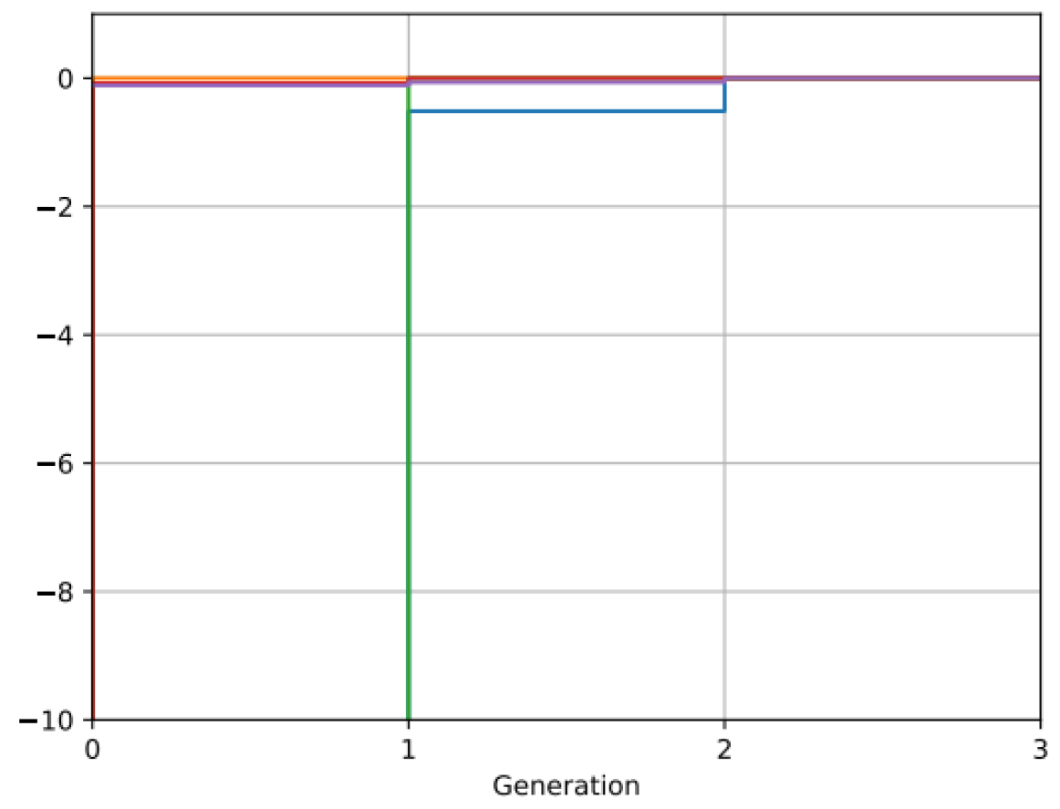
2.2. Evolutionary Optimisation

Evolutionary algorithms (EAs) are a class of metaheuristic algorithm that have become a widely adopted gradient-free, ‘global search’ optimisation tool. They can be categorised under the field of bioinspired optimisation, i.e., methods that draw inspiration from nature to mimic natural behaviours observed in nature [24]. Specifically, an EA replicates the biological mechanisms of evolution, natural selection and genetics [25]. Evolutionary algorithms often involve making changes to a ‘population’ of n individuals, often referred to as ‘agents’, evolving over number of ‘generations’.

Some examples of classifications of EAs are evolution programming (EP), evolution strategies (ESs), genetic programming (GP) and genetic algorithms (GAs) [26,27]. They follow similar methodologies, aiming to simulate the evolutionary process; however, they differ in their implementations [25]. An exhaustive review of genetic algorithms introduced between 1957 and 1993 demonstrates the rapid growth of the field [28].

One particular EA we used throughout the work presented in this paper is Particle Swarm Optimisation (PSO) [29] although the novel approach presented for exploiting area ruling to (cheaply) evaluate the objective function from the area distribution is equally applicable to all of the aforementioned optimisation strategies.

3. Methodology

The wave drag equation (Equation (3)) was used as the basis for defining the objective function given that the theoretical wave drag is proportional to the integral of the square of the second derivative of the area (note that in the EA literature the term ‘fitness function’ is often used interchangeably with ‘objective function’). In theory, wave drag can therefore be minimised by reducing the magnitude of the integral of the second derivative across the length of the body.

3.1. Objective Function

The objective function used in this work, J, is defined in Equation (5). This gives an indication of the ‘smoothness’ of the geometry’s longitudinal area distribution such that, according to Equation (1), minimising wave drag equates to minimisation of J. Throughout this work, 3D geometries were discretised using unstructured, surface meshes as typically used in CFD for two reasons:

• To allow direct comparison with full-fidelity CFD results using the same geometry description;
• To lend this approach to being used as the starting point in a CFD-based aerodynamic optimisation study (i.e., as a ‘cheap’, low-fidelity approach in the early stage of a design cycle).

The optimum geometry for a given baseline design and design space in each case is the mesh, M, with the lowest value of J.

$$J\left(M\right)={\int }_0^l{\left(S^{″}\left(x\right)\right)}^{2}dx$$

(5)

For a geometry parameterised using n independent design variables (parameters), $\mathit{\varphi }$$=\varphi ({\varphi }_1,{\varphi }_2,\dots ,{\varphi }_n)$, the optimisation problem is $min(J,M(\mathit{\varphi }\left)\right)$. Since the PSO algorithm, typically, is framed as a maximisation problem, the objective function in this work was negated. Note that the objective function J is sometimes referred to as the ‘smoothness’ of the geometry throughout this work, such that a low value of J implies a ‘smooth’ area distribution. The remainder of this section of the paper outlines the numerical scheme used to compute this objective function on a triangular surface mesh representation of a geometry.

3.2. Numerical Scheme

3.2.1. Area Computation

To calculate the area distribution of a given surface mesh, the Python module trimesh [30] was used to calculate the geometry cross-sectional area at intersection slices at user-defined locations. The trimesh module reads a watertight surface triangulation as input, so any hybrid meshes with quad elements were first passed through the Python module pyvista, which was used to triangulate a hybrid mesh as required.

The function section was used from the trimesh module, which returns the intersection curve between a given mesh and intersection plane. The object returned for the intersection curve also provides the area of this intersection slice as one of its built-in properties. Figure 2 shows an example of the intersection slice resulting at a particular x station along the length of the complex geometry case considered in this paper.

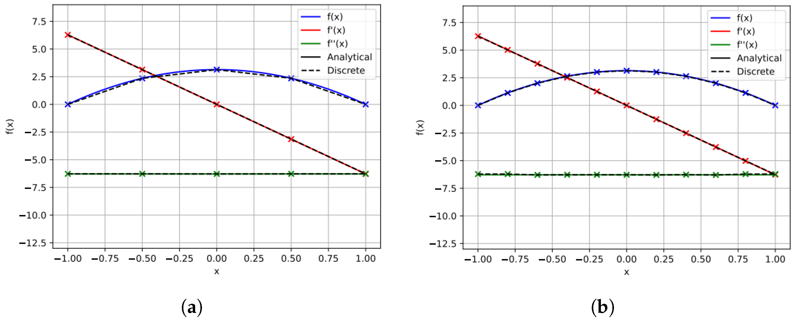
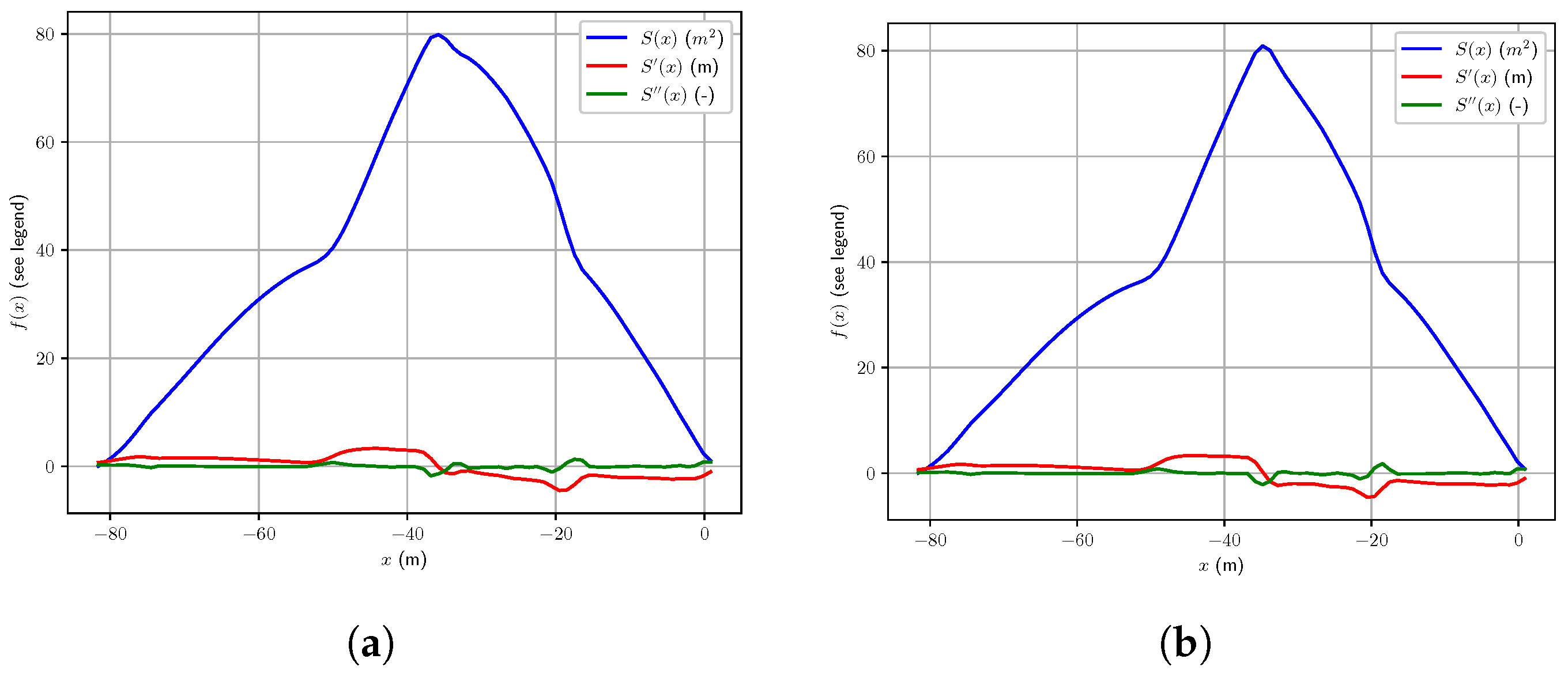
3.2.2. Differentiation

Second-order central differencing was used to calculate derivatives of S using Equation (6), where h represents the step size between uniformly distributed values of x. Boundary values were handled and compared using two different methods: extrapolating the domain using a constant, and using the forward difference (Equation (7)) and the backward difference (Equation (8)) where appropriate.

$$S^{\prime }\left(x\right)=\frac{S(x+h)-S(x-h)}{2h}$$

(6)

$$S^{\prime }\left(x\right)=\frac{-3S\left(x\right)+4S(x+h)-S(x+2h)}{2h}$$

(7)

$$S^{\prime }\left(x\right)=\frac{3S\left(x\right)-4S(x-h)+S(x-2h)}{2h}$$

(8)

The same treatment was used for second-order derivatives, for which the central, forward and backward difference stencils are shown in Equations (9), (10) and (11), respectively.

$$S^{″}\left(x\right)=\frac{S(x+h)-2S\left(x\right)+S(x-h)}{h^2}$$

(9)

$$S^{″}\left(x\right)=\frac{S(x+2h)-2S(x+h)+S\left(x\right)}{h^2}$$

(10)

$$S^{″}\left(x\right)=\frac{S\left(x\right)-2S(x-h)+S(x-2h)}{h^2}$$

(11)

3.2.3. Integration

For the implementations outlined in this paper, only integrals over one dimension are required. Therefore, the trapezium rule was used to approximate the integral in Equation (5) to determine the objective function.

3.3. Testing the Numerical Scheme

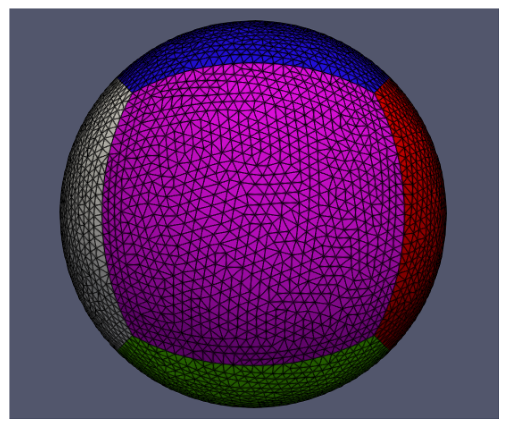
The practical implementation of the method outlined was explored in order to understand the numerical stability of the scheme on a variety of meshes. The effectiveness of this discrete implementation of area-distribution approximation was assessed using 3 test cases. The smoothness-driven optimisation procedure was then evaluated using a specific, complex geometry test case of particular interest to the authors: a single stage to orbit spaceplane being developed by Reaction Engines Ltd. [31], ‘Skylon’.

3.3.1. Sphere

The unit (m) radius sphere was used as the first test case because the analytical area distribution for this geometry is known and easy to calculate. The mesh-based geometry definition used is shown in Figure 3 with a mean cell size of 0.05 m. This cell size was chosen in order to provide a (qualitatively) reasonable geometric representation of the sphere. Clearly, as the cell size increases the quality of the geometric representation reduces and hence the effectiveness of the approach reduces; however, a detailed study into this was deemed beyond the scope of this work.

Figure 4 shows a comparison of the analytical solution and discrete (numerical) approximations for the area distribution and first and second derivatives of the area. It is clear that, for an extremely simple case such as this, when using just four slices the second derivative is calculated almost exactly whereas increasing the number of slices to 10 introduces some (minor) numerical error near the leading and trailing edges of the sphere. This simple example shows that it is therefore important to think carefully about how many slices to use, and where to position them, when applying the approach to more complex geometries as will be considered in the next sections.

3.3.2. Sears–Haack Body

A geometry with a more practical relevance to the topic of wave-drag and area-distribution analysis is the Sears–Haack body [21]. This is the body that gives the theoretical minimum wave drag for a given length and volume, or given radius at a fixed length. The analytical definition of the area distribution is known for this geometry and well studied. The analytical solutions for the distribution and derivatives are given in Figure 5a. The same mesh as used by Smith et al. [17] as their ‘coarse’ mesh example, with body maximum radius, $R_{max}=3.15$ m, was used as shown in Figure 5b.

Intersection planes (slices) were initially calculated in increments of 100, starting from 100. The RMSE of the discretised scheme compared to the analytical solution was calculated. From Figure 6a we can see that the RMSE increases significantly across this range and Figure 7a shows that this is due to the introduction of numerical fluctuations as early as 200 slices driven by the sensitivity to h (the distance between slices) of computing gradients as h becomes small.

The procedure was repeated, testing the number of slices within the range $[4,100]\subset \mathbb{N}$. The results from this are shown in Figure 6b where a smooth reduction in error up to 17 slices can be seen, after which it seems likely that numerical error is introduced. From here, the error increases unpredictably from this point, in a fashion similar to the coarser pass in Figure 6a. Unlike the clear numerical error shown when using 200 slices, the area-distribution derivatives in Figure 7b do not show significant numerical error and the discrete curve still matches very closely to the analytical solution. Most of the error in this example originates from the boundary calculations. This study, again, demonstrates the importance in the number (and location) of the slices used to compute the cross-sectional area.

Note that computationally this approach is so inexpensive (the 200-slice example running in under a second on a modern desktop PC) that the primary consideration is simply of appropriate number of slices to minimise the introduction of numerical error in the objective function computation rather than consideration of balancing accuracy against computational cost as would normally be the case.

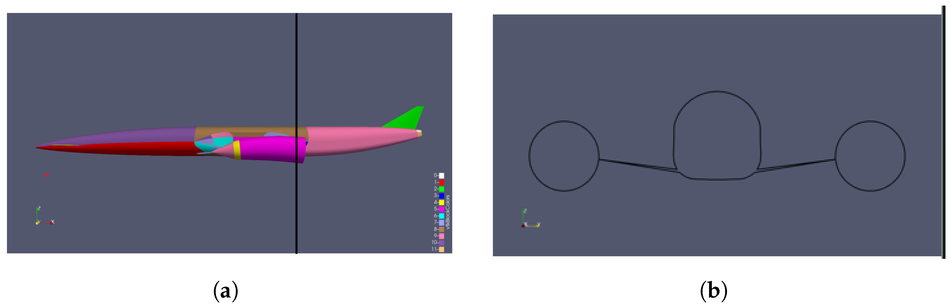
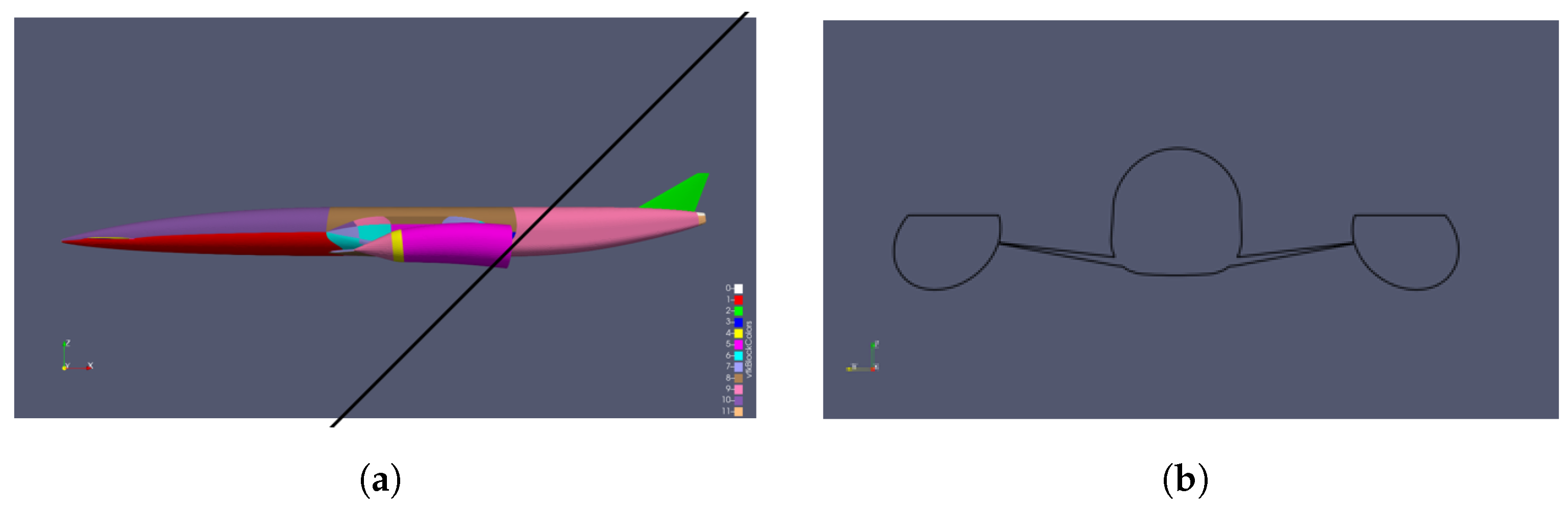
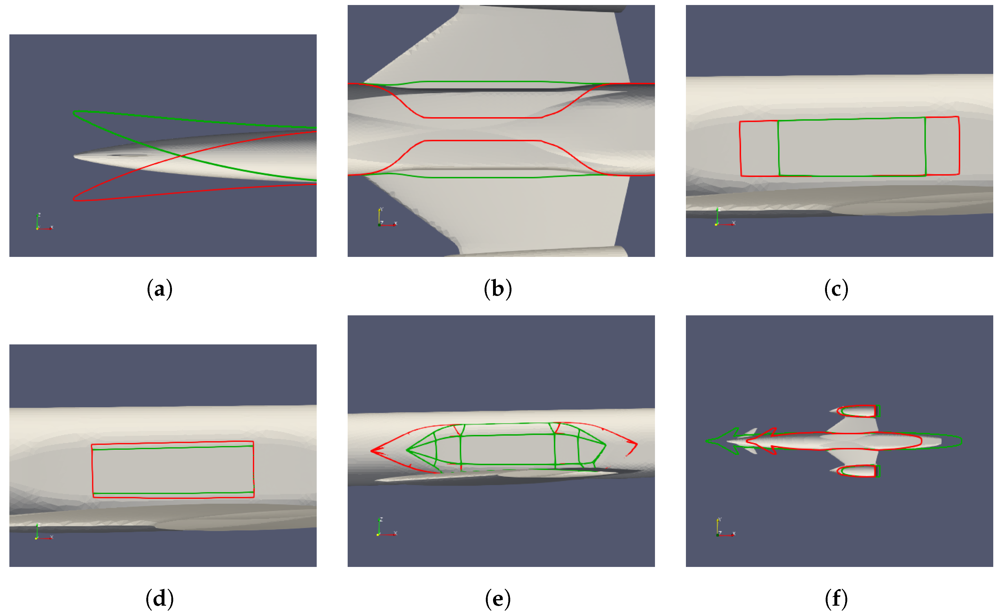
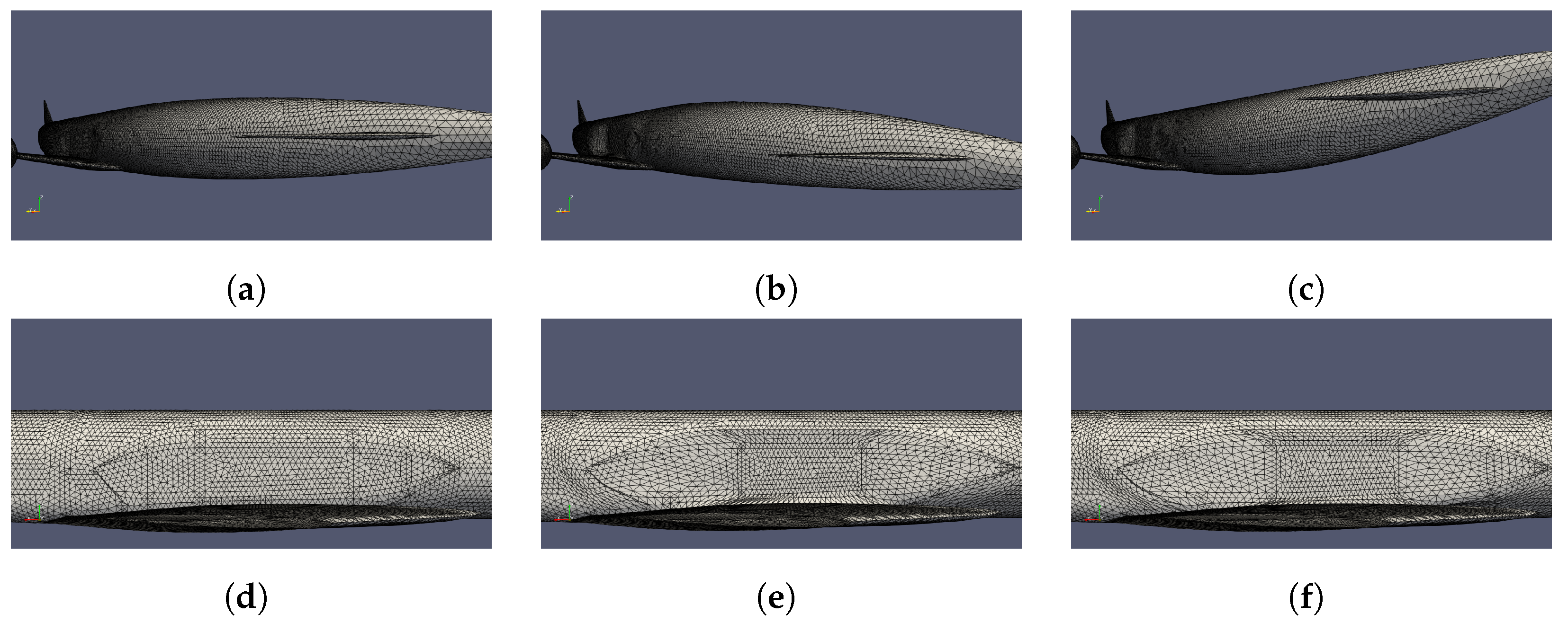
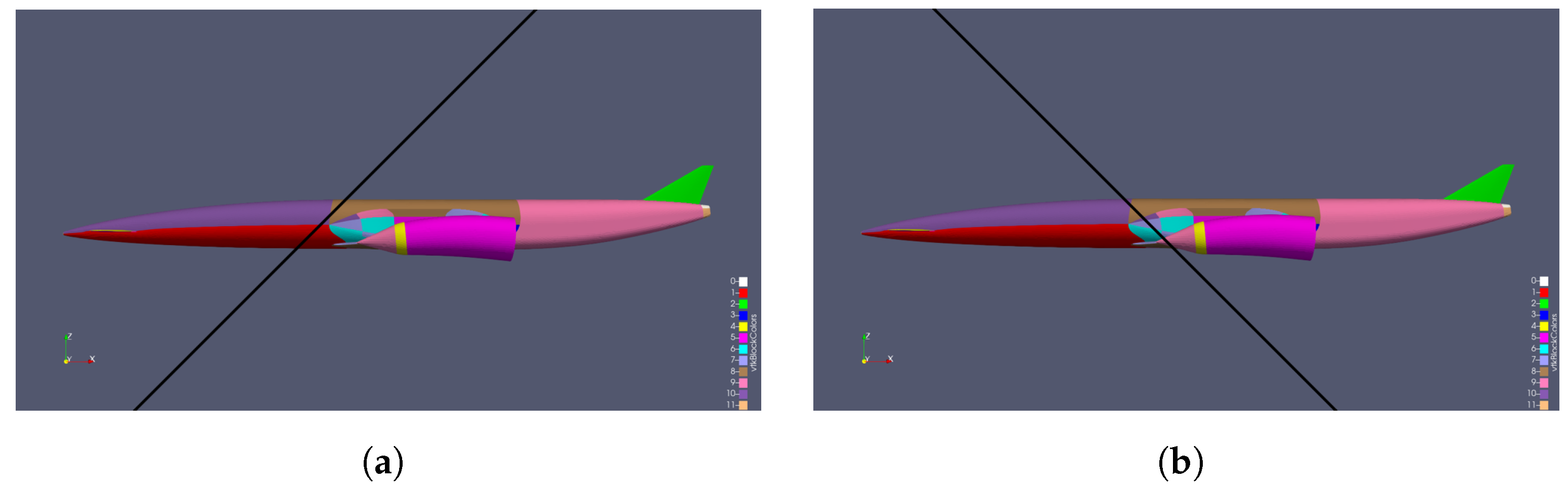
3.3.3. Complex Geometry—‘Skylon’ Spaceplane

Figure 8a shows the area distribution of the baseline Skylon geometry used in this work at $M=1.0$ using the method described in Section 3.2 with 80 slices along the length of the body. The significant difference in the cross-sectional areas between the slices before and after the end of the wings/nacelles at $x\approx -25$ results in a discontinuity in the cross-sectional area at this point. This has a signficant impact on the area-distribution smoothness calculation, with ‘spikes’ in $S^{″}\left(x\right)$ around this point. Increasing the number of slices by just 1 results in a decrease in magnitude of the spike (Figure 8b), while increasing the number of slices to 200 results in a steep increase in magnitude of the spike (Figure 8c). Distributions for 81 and 200 slices are shown in Figure 8. In the worst case of these examples, with 200 slices, the second derivative at this point dominates the smoothness calculation, J (Equation (5)).

The differences in the size of discontinuity between the different numbers of slices is due to the different locations along the length of the geometry at which the slices are taken. As the slices are uniformly distributed along the length, changing the number of slices changes the positions of the slices around the discontinuity in cross-sectional area. The slight changes in position in Figure 8a,b show how significant this effect can be on the numerical estimation of the second derivative of area and therefore the overall smoothness computation. Again, this reinforces the point about the importance of selecting appropriate locations for the intersection planes when using this discrete approach.

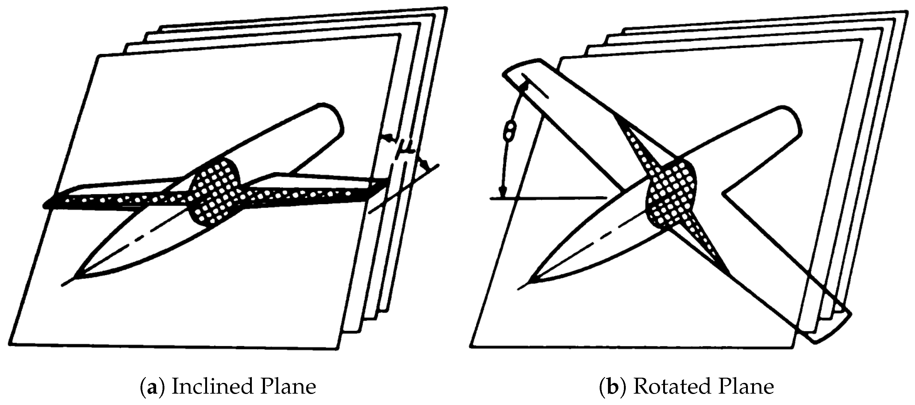
Mach Angle Inclination

When extending the transonic area rule at Mach 1 into the supersonic regime, the intersection planes used to slice the geometry must be inclined as described in Equation (2). At $M_{\infty }=1.2$, the resulting inclination angle $\mu =0.663$ radians. Figure 9 shows the area-distribution curves for the Skylon example when making this assumption.

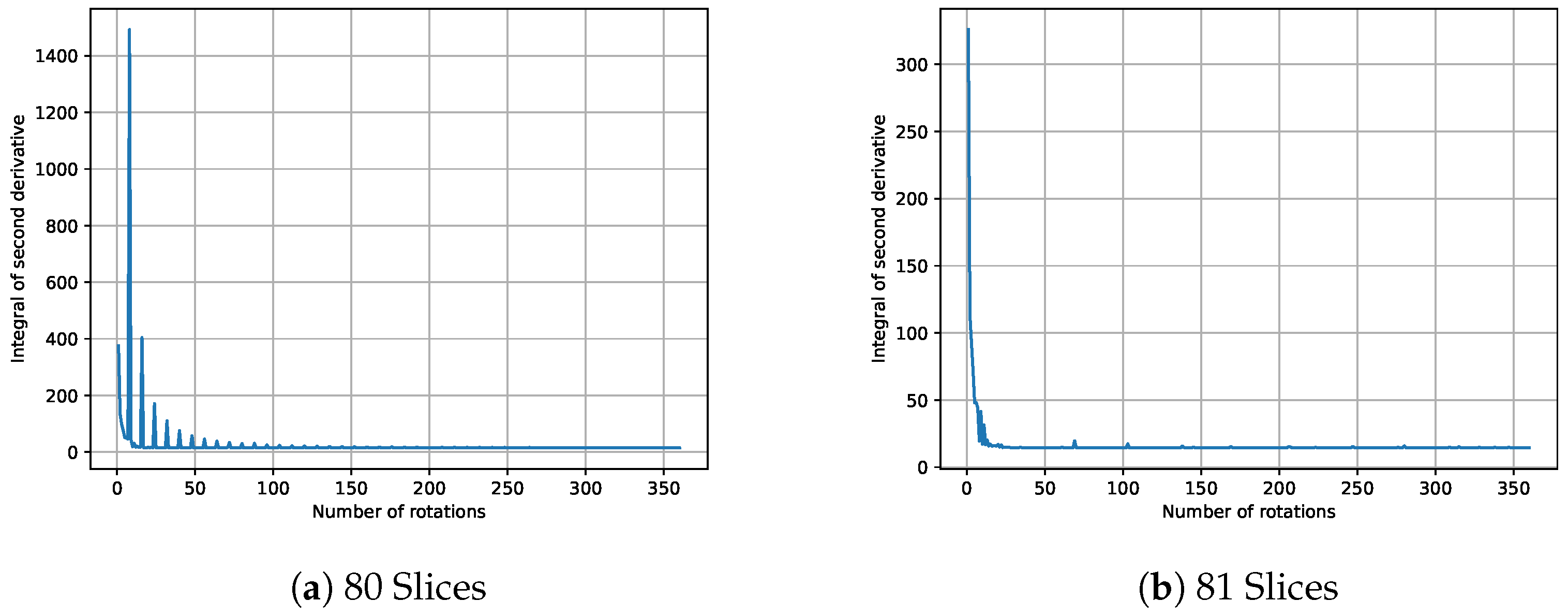
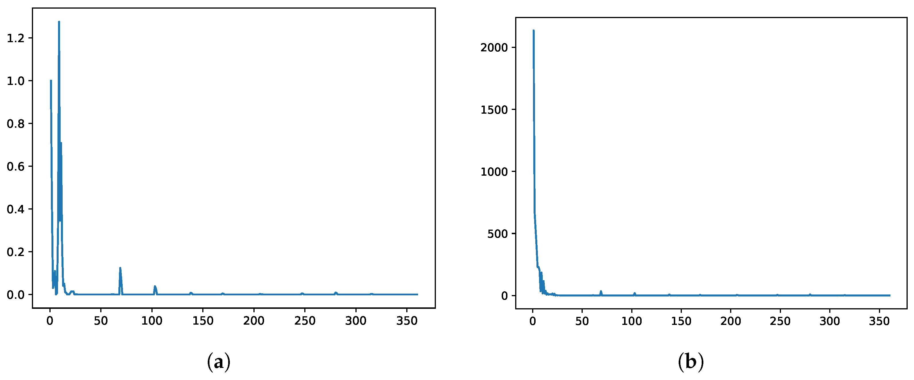
Inclination Plane Rotation

Rotation of the intersection plane, as shown in Figure 1, can reduce the effect of any discontinuities in the area distribution. The continuous integration can be handled discretely by averaging over n rotations. A sensible choice would be 360 rotations, at a rate of 1 slice per degree of rotation. A sensitivity study was conducted to determine approximately how many rotations should be made.

Initially, 80 slices were taken across the length of the body, with the number of rotations varying from 1 to 360, for which the convergence history of the geometry smoothness is shown in Figure 10a. The results exhibit numerous peaks that diverge significantly in value compared to their adjacent tests. Repeating this test with 81 slices instead results in the convergence history shown in Figure 10b in which the spikes, while still present, are significantly reduced in magnitude.

The main reason for running this convergence study was to determine whether increasing the number of rotations toward 360 resulted in the smoothness calculation converging. This is apparent from Figure 10b; however, computationally, this takes 360 times longer to calculate than with just one plane. Where computational resources are limited, it is beneficial to identify whether fewer rotations can be used and still achieve a similar value of smoothness. To determine this, the relative error from the previous number of rotations used and the absolute error compared to using 360 rotations is considered.

If the smoothness calculation with 360 rotational slices is taken as the ‘truth’ value, then the percentage error of this value is shown in Figure 11b. Using just 32 slices results in a difference of just $0.8\%$ and a relative error of using 31 slices of 2.3 × 10⁻⁵. This is a reasonable approximation, while taking significantly less time. Based on this, where computation time is of consequence, 32 slices can be used.

The reliability of using a coarser approximation with just 32 rotations can be qualitatively confirmed by comparing the area-distribution plots. Figure 12 shows the area-distribution plots when using 1, 4, 32 and 360 rotations. This figure highlights the differences between the plots when 4 and 360 slices are used, and the similarity between the plots when using 32 and 360 rotations.

As the number of lengthwise slices used has a clear impact on the calculation of the area-distribution smoothness, the analysis of all geometries within the optimisation procedure should be compared using the same number of lengthwise slices. It should be noted that, for some geometries, the selected value may not be the optimal value for that geometry and a large spike in smoothness may be erroneously calculated. All of the spikes lead to an increase in smoothness value, which could lead to a well-performing design being erroneously calculated to be a poorly performing design. This false negative may lead the optimiser to avoid some good designs. On the other hand, consider the scenario where the optimiser drives towards false positives. A false positive in this instance would be that a poor design is identified as a good design. This would be a significantly worse outcome.

Angle of Attack

So far, in all cases presented, it has been assumed that the angle of attack is 0, i.e., the flow is aligned with the x-axis. The comparative CFD-driven optimisation studies, taken from [17], were subject to a lift constraint at an angle of attack of $4^{\circ }$. The handling of this is included in Jones’ report [15] such that the normal of the interception plane should be parallel to the incoming stream.

The impact of including the additional plane inclination in the area-distribution curve calculation can be seen by comparing the distributions for the baseline design at 0 and 4 degrees angles of attack, Figure 13. Although subtle, the changes in area distribution resulting from the intersection plane angle change required to account for body of angle of attack is significant ($34\%$ in the case shown).

4. Optimisation Results

The Sears–Haack body was not used as a baseline geometry for an optimisation case given that it is already an optimal shape. The following sections detail the results when using the unit sphere (simple geometry case) and Skylon spaceplane (complex geometry case) as a baseline for a drag-minimisation optimisation study.

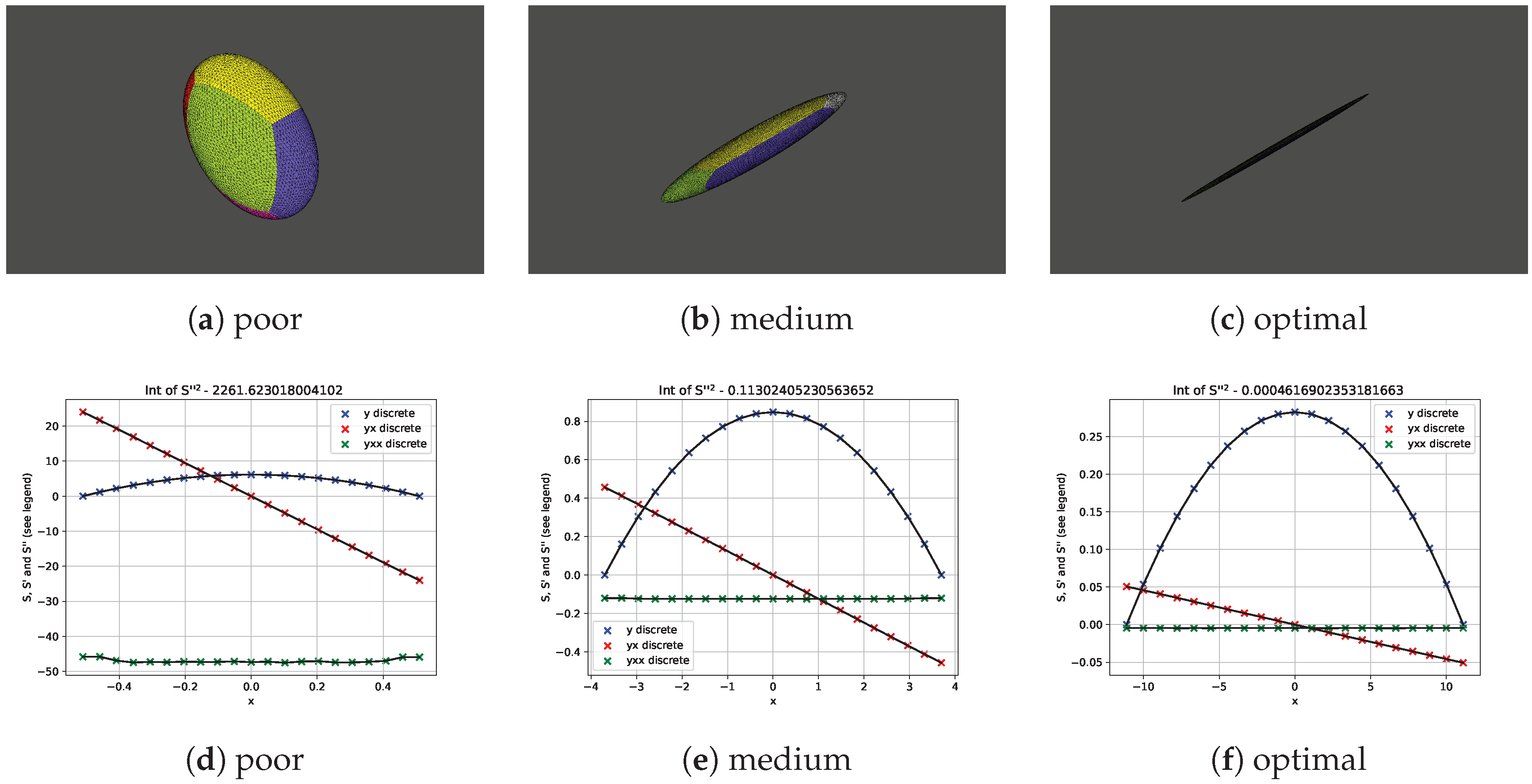
4.1. Simple Geometry—Sphere

The objective of the optimisation was wave-drag minimisation at Mach 1 and the problem was prescribed to be volume constrained. The expected outcome of the study was that the geometry should tend towards that of a slender, Sears–Haack type shape to the extent that the geometry parameterisation allowed. The geometry parameterisation and surface mesh morphing approach taken from Smith et al. [17] were used with a maximum perpendicular radius of the geometry (perpendicular to the x-axis, aligned with the flow direction) used as the single independent design parameter. The length of the geometry was then adjusted in order to ensure the body’s volume was conserved.

The bounds chosen for the longitudinal scaling were $\varphi \in [0.3,1.5]$ m (with $\varphi =1.0$ m as the baseline) and the PSO algorithm was used with five particles for four generations. The convergence history for this case is shown in Figure 14 and clearly the optimisation process is driving the geometry towards a minimum J solution. Within this short (and expensive) optimisation run, the algorithm converged to an optimal solution with $\varphi =0.3$ m, i.e., the most slender geometry possible, as expected. Comparing geometries, Figure 15b,c, we can see that, qualitatively, the optimal design tends toward the slender Sears–Haack shape, as expected, to the extent possible using this simple parameterisation approach. This simple case provided confidence in the scheme’s ability to provide sensible, minimum-wave-drag solutions and was therefore next tested with a complex geometry example.

4.2. Complex Geometry—Skylon Spaceplane

The aim of this test case was to achieve wave-drag minimisation on a much more complex and realistic aerospace vehicle geometry and to compare the results with CFD-driven optimisation. The same parameterisation approach, design space construction, mesh morphing and initial sampling as used by Smith et al. [17], was used. The geometry parameterisation approach is shown in Figure 16 where five independent design parameters $({\varphi }_1,{\varphi }_2,{\varphi }_3,{\varphi }_4$ and ${\varphi }_5)$ were used to define the design space and a sixth dependent parameter, ${\varphi }_c$, was used to enforce the volume conservation constraint. The area distribution for each geometry was calculated at $M_{\infty }=1.2$ and the angle of attack at $\alpha ={4.0}^{\circ }$.

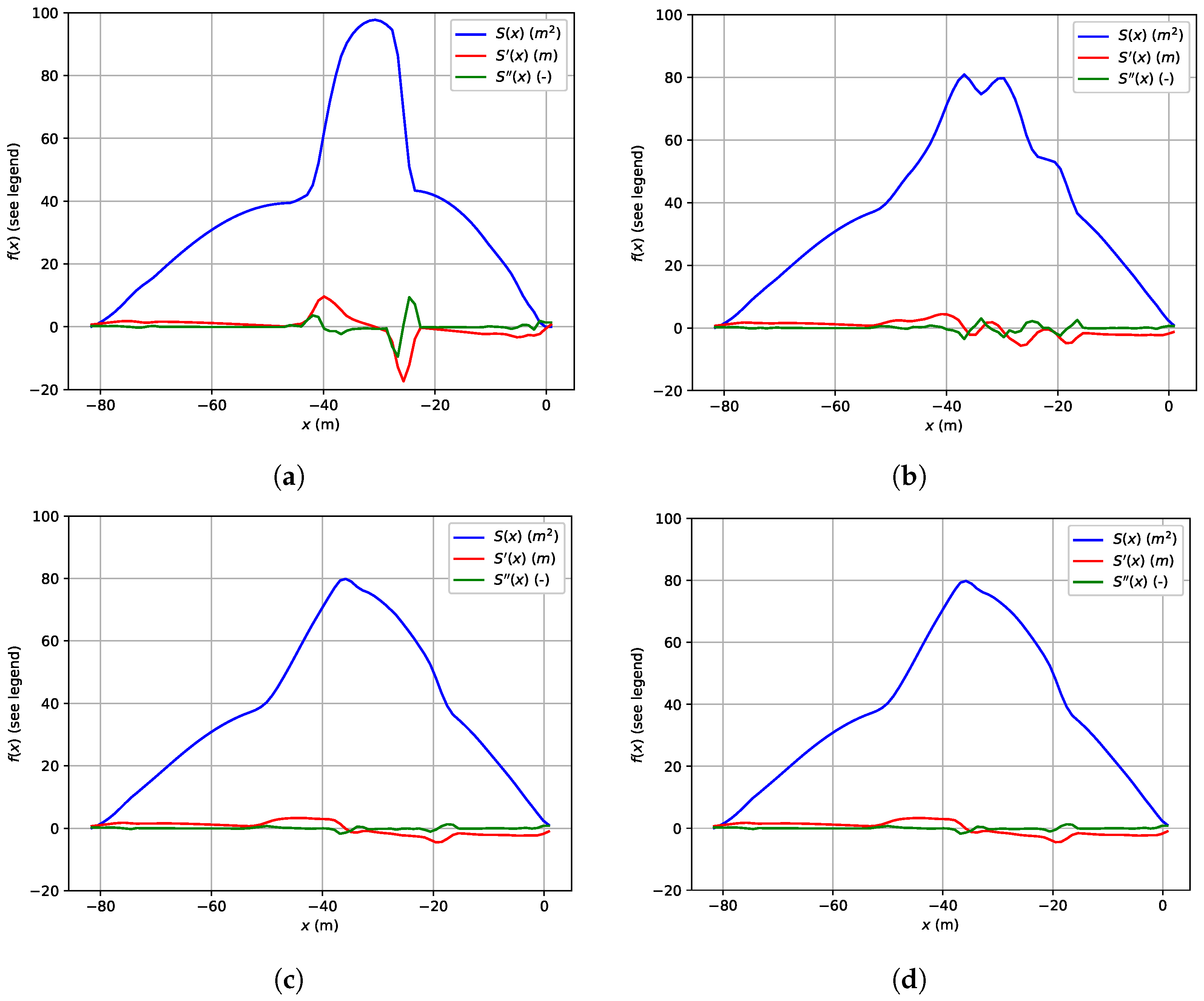
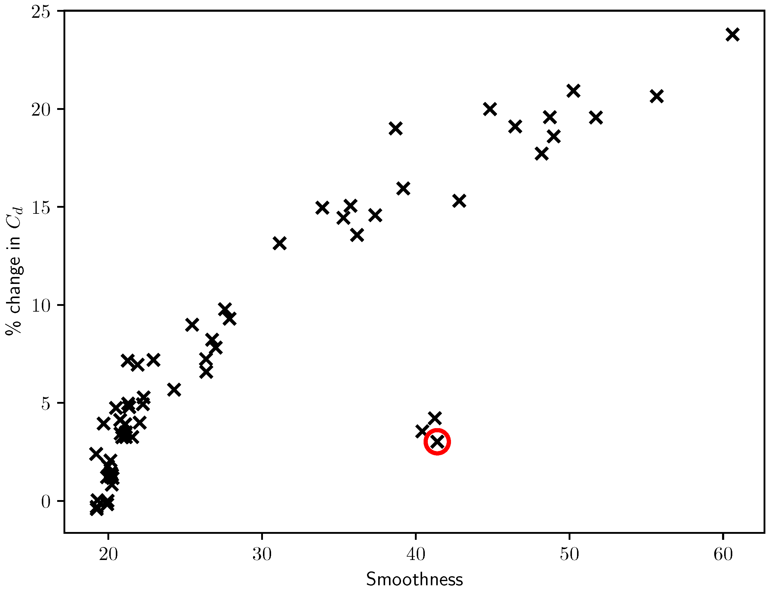
4.2.1. Direct Comparison of Area Distribution and CFD Predictions of $C_d$

The average of 32 rotated slices was taken at each of 81 slices in the x-direction x (along the length of the body). The resulting smoothness, Equation (5), for each geometry was compared against the percentage change from the baseline design. This correlation is shown in Figure 17 where there is a clear relationship between the CFD-free and CFD-based approaches. The Spearman rank coefficient between the two data sets was 0.909. This suggested that using the area distribution to approximate the actual objective function would result in a pattern of results similar to that when using full-fidelity CFD. There were, however, some outliers (three cases as seen in Figure 17) and each of these corresponded to geometries where an intersection slice location coincided with a discontinuity in the cross-sectional area distribution (as described previously). This, once again, reinforces the point made previously about being careful about the location of intersection slices.

4.2.2. Optimisation Case 1

For the first case, the area distribution was not calculated by rotating the plane about the x-axis but the plane was tilted by the angle $\mu$. This was performed to reduce the computational cost but still reduce the impact of the singularities in the second derivative around the engine inlets/outlets.

The optimisation algorithm used was PSO with 10 particles for 20 generations. The convergence history, Figure 18, shows that the algorithm converged on a design that maximises the smoothness (i.e., minimises J, Equation (5)).

Comparing with the results of Smith et al. [17], which used a CFD-driven optimisation, shown in Figure 19, the wasted, ‘pinch’ centre panel tends towards the same configuration in both cases. Aerodynamically this is happening to satisfy the basic principles of ‘area ruling’ [16]. However, the nose droop position differs significantly in that the CFD-driven optimisation tends towards designs where the nose is drooped down, whereas the CFD-free-driven optimisation tends towards designs where the nose is drooped upwards, which is counter to what we would expect to see for this study.

It was postulated that the cause of this discrepancy is due to the fact that this initial study used a single inclined plane at each station x rather than rotating around the axis and possibly some contribution from numerical error in the area-distribution calculations. Designs where the nose of the geometry is angled to point in the same direction as the normal of the plane have lower values of smoothness in area distribution at this point which will reflect positively in the evaluation function. If this is the case, then we would expect that changing the angle of the plane would impact the results of the study or, equally, calculating the area distribution using the full rotation around the axis should average this impact out of the optimisation.

We explore both of these predictions separately in the following sections.

4.2.3. Optimisation Case 2—Changing the Angle of the Slice Plane

It was postulated that the optimisation procedure outlined above directly led to raising the nose of the geometry due to the angle of the Mach plane. Therefore, repeating the same optimisation procedure but with a plane inclined negatively along the axis should result in similar designs being obtained, but with the nose droop trending downwards. Figure 20 demonstrates what is implied by the negation of the inclination angle.

Figure 21 shows the area-distribution curves for the same geometries as in Figure 22 except that the inclination plane was calculated at a negative angle to the x-axis.

We can indeed see from this a different trend in the calculation of the smoothness of the area distribution. The convergence history with this negated angle of inclination, $\mu$, is shown in Figure 23 which has a very similar pattern to that in Figure 18 implying a similar reduction in drag but, in this case, the nose droop trended downwards.

4.2.4. Optimisation Case 3—Averaging the Rotation of the Slice Plane

Case 1 was also repeated but by calculating the area distribution as the average of rotated planes. We evaluated the area distribution using 360 averaged rotation planes. Figure 24 shows the convergence history from this study and the optimal design resulting is shown in Figure 25.

These results confirm the postulation made prior to the study that rotation of the intersection plane averages out any contribution from the nose droop. The optimal design, shown in Figure 25b, from this study, when compared to that of the previously un-rotated study in Figure 19c, has a negligible droop while exhibiting similar wasting around the central pinch panel to other optimal designs, Figure 25a.

4.2.5. Angle of Attack

The final condition that needs to be included in the calculation of the area distribution is to account for the angle of attack. Inclining the plane so that the plane normal faces into the freestream, as discussed in Section 2, achieves this. The area-distribution-driven optimisation was repeated, again performing the complete rotation of the plane around the x-axis. The convergence history for the CFD-free PSE optimisation for this is shown in Figure 26.

The optimal result from this study is shown in Figure 27 where it is clear that the nose droop has been impacted by this approach and is angled downwards towards the theoretical freestream flow. The effect on the central ‘pinch’ panel remains largely the same.

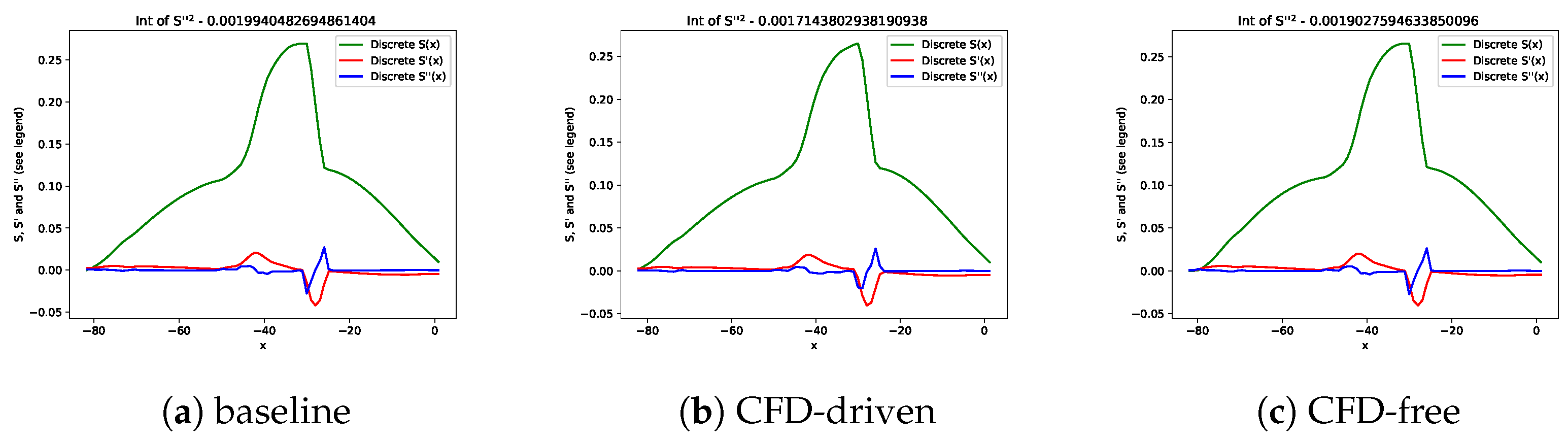
4.3. Optimal Design Analysis

Using the geometry smoothness instead of CFD to drive the objective function of the optimisation procedure results in qualitatively very similar designs. In both cases (CFD-driven and CFD-free), the nose is drooped down and the central side panel is pinched in towards the payload bay. Quantitatively, it was not possible to directly compare the $C_d$ reduction achieved using this method with the CFD-driven approach of Smith et al. [17] since in their work there was the additional constraint of fixing the lift generated. This constraint cannot be implemented using the methodology outlined in this paper.

However, it is interesting to note that the the optimised design (from case 3 at $4^{\circ }$ angle of attack) was $1.2\%$ below the baseline geometry compared with the reduction of $1.6\%$ achieved by the CFD-driven study [17] (where the angle of attack was altered to fix the lift). This is impressive considering the seconds of compute time necessary on a desktop PC for the CFD-driven approach compared with many hundreds of CPU-hours on an HPC system required for the CFD-driven study.

5. Conclusions and Recommendations

An innovative, CFD-free approach for wave-drag-minimising optimisation problems for 3D geometries defined on ‘typical’ surface mesh triangulations has been presented. The approach takes advantage of the basic and fundamental principles of ‘area ruling’. The approach presented has been shown to be effective as an extremely cheap, even though somewhat crude, method for guiding an optimiser towards a sensible drag-minimising design for problems where wave drag dominates. Although effective, it is clear that this approach cannot completely replace a classical CFD-driven aerodynamic optimiser as it is incapable of handling complex, non-geometry based constraints, involving aerodynamic loads other than wave drag (e.g., lift constraints). This study demonstrates the importance of the placement of the intersection slices used to compute a geometry’s area distribution and further work is recommended to develop an automated algorithm to suggest the appropriate placement of these intersection slices. Also, since this paper aimed simply to prove the principle of this approach, mesh resolution sensitivity studies for each case were deemed beyond the scope of study. The authors recommend that, in future, if adopting the approaches outlined here the usual mesh sensitivity analysis should be carried out to determine the appropriate grid resolution.

Despite its limitations, it is recommended that this approach could be used as a very efficient and effective method for the early stages of an optimisation process on complex geometries before switching to the more computationally intensive CFD-driven schemes more commonly used which can take into account a broader range of factors (including other drag terms and phenomena such as flow separation).

References

1. Jameson, A.; Vassberg, J. Computational fluid dynamics for aerodynamic design-Its current and future impact. In Proceedings of the 39th Aerospace Sciences Meeting and Exhibit, Reno, NV, USA, 8–11 January 2001; p. 538. [Google Scholar]
2. Jameson, A. Efficient aerodynamic shape optimization. In Proceedings of the 10th AIAA/ISSMO Multidisciplinary Analysis and Optimization Conference, Albany, NY, USA, 30 August–1 September 2004; p. 4369. [Google Scholar]
3. Vassberg, J.C.; Jameson, A. Aerodynamic shape optimization of a Reno race plane. Int. J. Veh. Des. 2002, 28, 318–338. [Google Scholar] [CrossRef]
4. Quagliarella, D.; Vicini, A. Viscous single and multicomponent airfoil design with genetic algorithms. Finite Elem. Anal. Des. 2001, 37, 365–380. [Google Scholar] [CrossRef]
5. Naumann, D.S.; Evans, B.; Walton, S.; Hassan, O. A novel implementation of computational aerodynamic shape optimisation using modified cuckoo search. Appl. Math. Modell. 2016, 40, 4543–4559. [Google Scholar] [CrossRef]
6. Naumann, D.; Evans, B.; Walton, S.; Hassan, O. Discrete boundary smoothing using control node parameterisation for aerodynamic shape optimisation. Appl. Math. Modell. 2017, 48, 113–133. [Google Scholar] [CrossRef]
7. Marsden, A.L.; Wang, M.; Dennis, J.E.; Moin, P. Suppression of vortex-shedding noise via derivative-free shape optimization. Phys. Fluids 2004, 16, L83–L86. [Google Scholar] [CrossRef]
8. Walton, S.; Hassan, O.; Morgan, K.; Brown, M.R. Modified cuckoo search: A new gradient free optimisation algorithm. Chaos Solitons Fractals 2011, 44, 710–718. [Google Scholar] [CrossRef]
9. Skinner, S.N.; Zare-Behtash, H. State-of-the-art in aerodynamic shape optimisation methods. Appl. Soft Comput. 2018, 62, 933–962. [Google Scholar] [CrossRef]
10. Giannakoglou, K.C.; Papadimitriou, D.I.; Kampolis, I.C. Aerodynamic shape design using evolutionary algorithms and new gradient-assisted metamodels. Comput. Meth. Appl. Mech. Eng. 2006, 195, 6312–6329. [Google Scholar] [CrossRef]
11. Periaux, J.; Lee, D.S.; Gonzalez, L.F.; Srinivas, K. Fast reconstruction of aerodynamic shapes using evolutionary algorithms and virtual nash strategies in a CFD design environment. J. Comput. Appl. Math. 2009, 232, 61–71. [Google Scholar] [CrossRef]
12. Secco, N.R.; Kenway, G.K.; He, P.; Mader, C.; Martins, J.R.R.A. Efficient mesh generation and deformation for aerodynamic shape optimization. AIAA J. 2021, 59, 1151–1168. [Google Scholar] [CrossRef]
13. Ahmad, N.E.; Abo-Serie, E.; Gaylard, A. Mesh optimization for ground vehicle aerodynamics. CFD Lett. 2010, 2, 54–65. [Google Scholar]
14. Biancolini, M.E.; Viola, I.M.; Riotte, M. Sails trim optimisation using CFD and RBF mesh morphing. Comp. Fluids 2014, 93, 46–60. [Google Scholar] [CrossRef]
15. Jones, R.T. Theory of Wing-Body Drag at Supersonic Speeds; Technical Report; NASA: Washington, DC, USA, 1956.
16. Whitcomb, R.T. A Study of the Zero-Lift Drag-Rise Characteristics of Wing-Body Combinations Near the Speed of Sound; Technical Report; NASA: Washington, DC, USA, 1956.
17. Smith, B.; Evans, B.; Walton, S. A Novel Mesh Morphing Methodology for Computational Aerodynamic Shape Optimisation. Under Rev. Comp. Struct. 2024, 40, 4543–4559. [Google Scholar] [CrossRef]
18. Armenta, F.X.; Takahashi, T.T. Revisiting the Transonic Area Rule for Conceptual Aerodynamic Design. In Proceedings of the AIAA Aviation 2021 Forum, Virtual, 2–6 August 2021; p. 2441. [Google Scholar]
19. Ashley, H.; Landahl, M.; Landahl, M.T. Aerodynamics of Wings and Bodies; Courier Corporation: North Chelmsford, MA, USA, 1965. [Google Scholar]
20. Haack, W. Geschossformen kleinsten wellenwiderstandes. Ber. Lilienthal-Ges. 1941, 136, 14–28. [Google Scholar]
21. Sears, W.R. On projectiles of minimum wave drag. Q. Appl. Math. 1947, 4, 361–366. [Google Scholar] [CrossRef]
22. Lomax, H.; Heaslet, M.A. Recent developments in the theory of wing-body wave drag. J. Aeronaut. Sci. 1956, 23, 1061–1074. [Google Scholar] [CrossRef]
23. Harris, R.V., Jr. An Analysis and Correlation of Aircraft Wave Drag; National Aeronautics and Space Administration: Washington, DC, USA, 1964.
24. Yang, X.S. Nature-Inspired Metaheuristic Algorithms; Luniver Press: Bristol, UK, 2010. [Google Scholar]
25. Back, T.; Hammel, U.; Schwefel, H.P. Evolutionary computation: Comments on the history and current state. IEEE Trans. Evol. Comput. 1997, 1, 3–17. [Google Scholar] [CrossRef]
26. Bartz-Beielstein, T.; Branke, J.; Mehnen, J.; Mersmann, O. Evolutionary algorithms. Wiley Interdiscip. Rev. Data Min. Knowl. Discovery 2014, 4, 178–195. [Google Scholar] [CrossRef]
27. Vikhar, P.A. Evolutionary algorithms: A critical review and its future prospects. In Proceedings of the 2016 International Conference on Global Trends in Signal Processing, Information Computing and Communication (ICGTSPICC), Jalgaon, India, 22–24 December 2016; pp. 261–265. [Google Scholar]
28. Alander, J.T. An Indexed Bibliography of Genetic Algorithms: Years 1957–1993; Citeseer: Princeton, NJ, USA, 1994. [Google Scholar]
29. Kennedy, J.; Eberhart, R. Particle swarm optimization. In Proceedings of the ICNN’95-International Conference on Neural Networks, Perth, WA, Australia, 27 November–1 December 1995; Volume 4, pp. 1942–1948. [Google Scholar]
30. Trimesh. Available online: https://github.com/mikedh/trimesh (accessed on 1 March 2024).
31. Reaction Engines Ltd. Available online: https://reactionengines.co.uk/ (accessed on 1 March 2024).
Figure 2. Intersection plane cutting through a spaceplane geometry and the intersection curve/slice between the geometry and the plane. (a) Side view with plane location. (b) Cross-sectional intersection.
Aerospace 11 00298 g002
Figure 3. Unstructured, triangular mesh used to define the geometry of a unit (m) radius sphere. Mean triangle (cell) size is 0.05 m.
Aerospace 11 00298 g003
Figure 4. Comparison between analytical and discrete area distributions (and derivatives) for a sphere using 4 and 10 slices. (a) Four slices; (b) ten slices.
Aerospace 11 00298 g004
Figure 5. Analytical solution of the area distribution, its derivatives and example 3D mesh of the Sears–Haack body with parameters R m a x = 3.15 m and l = 81.0 m. (a) Cross-sectional area distribution; (b) 3D surface mesh.
Aerospace 11 00298 g005
Figure 6. RMSE as a function of number of discrete intersection slices taken over the length of the body. (a) Increasing in steps of 100, starting from 100; (b) increasing in steps of 1, starting from 4.
Aerospace 11 00298 g006
Figure 7. Two examples of the discretised calculation of first and second derivatives of the area distribution for a Sears–Haack body compared with the analytical solutions. (a) uses 200 slices and it can be clearly seen around x = 43 that there is significant numerical error. (b) uses just 20 slices and is qualitatively very close to the exact solution except at the boundaries.
Aerospace 11 00298 g007
Figure 8. Area-distribution plot for the Skylon spaceplane using varying numbers of slices along the length of the geometry, calculate at conditions M = 1.0 , α = 0.0 : (a) 80 slices; (b) 81 slices; (c) 200 slices.
Aerospace 11 00298 g008
Figure 9. Mach plane cutting through the Skylon geometry inclined at Mach 1.2 and the slice this cut makes. (a) Side view with plane location; (b) cross-sectional intersection.
Aerospace 11 00298 g009
Figure 10. Comparison between the convergence of the area-distribution smoothness computation, J, with number of rotations for 80 (a) and 81 (b) lengthwise slices.
Aerospace 11 00298 g010
Figure 11. Relative error from previous iteration (a) and percentage error compared with using 360 rotations (b) using 81 slices along the length of the Skylon geometry. (a) Relative error; (b) absolute error.
Aerospace 11 00298 g011
Figure 12. Area-distribution calculations for the baseline Skylon design using varying numbers of rotational planes: (a) 1 rotational plane; (b) 4 rotational planes; (c) 32 rotational planes; (d) 360 rotational planes.
Aerospace 11 00298 g012
Figure 13. The area-distribution curves and derivatives for the baseline Skylon geometry at varying angles of attack, α . While the distributions are visually very similar, a clear difference in the shape of the peak in the range 40 x 20 can be seen. There is also a significant difference in the smoothness; J = 14.70 at α = 0 and J = 19.71 at α = 4 , a 34 % difference. (a) α = 0 ; (b) α = 4 .
Aerospace 11 00298 g013
Figure 14. Convergence history of sphere drag optimisation case showing evolution of J (y-axis) against generation number for 5 PSO particles across 4 generations. This case has a single independent (design) parameter (axial radius) and one dependent parameter (body length) used to enforce the volume constraint. Note that the y-axis range is cropped.
Aerospace 11 00298 g014
Figure 15. Geometries (ac) and area distributions (df) of three different designs from the simple sphere optimisation case. Considering the limited design space, a poor design (a), good design (b) and optimal design (c) are shown.
Aerospace 11 00298 g015
Figure 16. Bounds for parameterised Skylon geometry. (ae) show the bounds for independent (design) parameters ϕ 1 ϕ 5 . The dependent parameter, ϕ c , was used to constrain the volume, shown in (f) [17]. (a) ϕ 1 ‘nose droop’; (b) ϕ 2 fuselage ‘pinching’; (c) ϕ 3 centre panel length; (d) ϕ 4 centre panel height; (e) ϕ 5 overall ‘pinch’ length; (f) ϕ c fuselage length.
Aerospace 11 00298 g016
Figure 17. Correlation between full-fidelity (CFD) prediction of drag increase and the area-distribution approach proposed in this study for a sample size of 60 (using Latin Hypercube Sampling). Eighty-one lengthwise slices were used for each geometry and there are three clear outliers.
Aerospace 11 00298 g017
Figure 18. Convergence history for a PSO optimisation study using the area distribution in the cost function evaluation.
Aerospace 11 00298 g018
Figure 19. Front and side images of the morphed surface mesh for the baseline design, optimal design from the CFD-driven optimisation study [17] and the ‘Case 1’ CFD-free approach proposed in this paper. (a) Baseline—front; (b) CFD-driven—front; (c) CFD-free—front; (d) baseline—side; (e) CFD-driven—side; (f) CFD-free—side.
Aerospace 11 00298 g019
Figure 20. Inclined Mach planes with a positive inclination angle, μ (a), and negative inclination angle, μ (b).
Aerospace 11 00298 g020
Figure 21. Area-distribution plots where the Mach plane is inclined negatively with respect to the x-axis for the baseline design (a), the optimal design from the Bayesian study (b) and the initial PSO optimised study driven by the area distribution (c).
Aerospace 11 00298 g021
Figure 22. Area-distribution plots for the baseline design, the CFD-driven optimisation study [17] and the ‘Case 1’ CFD-free approach proposed in this paper. (a) Baseline; (b) CFD-driven; (c) CFD-free.
Aerospace 11 00298 g022
Figure 23. Convergence history for a PSO optimisation study using the area distribution in the cost function evaluation with the slice plane inclined at a negative inclination angle μ .
Aerospace 11 00298 g023
Figure 24. Convergence history for the Skylon optimisation with CFD-free PSO using 10 particles over 20 generations using 360 averaged rotation planes.
Aerospace 11 00298 g024
Figure 25. Front and side images of the morphed surface mesh optimal design when the area-distribution calculation uses intersection plane rotation. (a) Side; (b) front.
Aerospace 11 00298 g025
Figure 26. Convergence history for the Skylon optimisation using PSO using 10 particles over 20 generations. The objective function used the area-distribution calculation including the averaged rotation of the inclined Mach plane with angle of attack correction.
Aerospace 11 00298 g026
Figure 27. Front and side profiles (right) and area distribution (left) for the optimal design following area-distribution-driven optimisation including an angle of attack. (a) Front; (b) side; (c) area distribution.
Aerospace 11 00298 g027
Disclaimer/Publisher’s Note: The statements, opinions and data contained in all publications are solely those of the individual author(s) and contributor(s) and not of MDPI and/or the editor(s). MDPI and/or the editor(s) disclaim responsibility for any injury to people or property resulting from any ideas, methods, instructions or products referred to in the content.